HAL Id: hal-00317416
https://hal.archives-ouvertes.fr/hal-00317416
Submitted on 14 Jun 2004
HAL is a multi-disciplinary open access
archive for the deposit and dissemination of
sci-entific research documents, whether they are
pub-lished or not. The documents may come from
teaching and research institutions in France or
abroad, or from public or private research centers.
L’archive ouverte pluridisciplinaire HAL, est
destinée au dépôt et à la diffusion de documents
scientifiques de niveau recherche, publiés ou non,
émanant des établissements d’enseignement et de
recherche français ou étrangers, des laboratoires
publics ou privés.
Comparison of high latitude electron density profiles
obtained with the GPS radio occultation technique and
EISCAT measurements
C. Stolle, N. Jakowski, K. Schlegel, M. Rietveld
To cite this version:
C. Stolle, N. Jakowski, K. Schlegel, M. Rietveld. Comparison of high latitude electron density profiles
obtained with the GPS radio occultation technique and EISCAT measurements. Annales Geophysicae,
European Geosciences Union, 2004, 22 (6), pp.2015-2022. �hal-00317416�
© European Geosciences Union 2004
Geophysicae
Comparison of high latitude electron density profiles obtained with
the GPS radio occultation technique and EISCAT measurements
C. Stolle1, N. Jakowski2, K. Schlegel3, and M. Rietveld3,4
1Institute for Meteorology, University of Leipzig, Stephanstr. 3, 04103 Leipzig, Germany
2Institute of Communications and Navigation, DLR Neustrelitz, Kalkhorstweg 53, 17235 Neustrelitz, Germany 3Max-Planck-Institut f¨ur Aeronomie, Max-Planck-Str. 2, 37191 Katlenburg-Lindau, Germany
4EISCAT, Ramfjordmoen, 9027 Ramfjordbotn, Norway
Received: 21 July 2003 – Revised: 21 January 2004 – Accepted: 9 February 2004 – Published: 14 June 2004
Abstract. To obtain a comprehensive view on high latitude
processes by applying different observation techniques, the SIRCUS campaign was initiated in 2001/2002. This paper compares electron density profiles derived from CHAMP ra-dio occultation data and those measured with the EISCAT facility. Since ionospheric profiling with the help of space-based received GPS is a relatively new technique, validations with established independent instruments are of crucial need. We present 28 profiling events for quasi-statistical analyses, which occurred during the SIRCUS campaigns and describe some of them in more detail. We found out that the major-ity of profile comparisons in electron densmajor-ity peak value and height, as well as in TEC, lie within the error ranges of the two methods. Differences in the ionospheric quantities do not necessarily occur when the locations of the occultation and of the radar site show considerable distances. Differ-ences are more pronounced when the ionosphere is remark-ably structured.
Key words. Radio science (Remote sensing), Ionosphere
(Polar ionosphere, instruments and techniques)
1 Introduction
One aim of the SIRCUS (Satellite and Incoherent scatter Radar Cusp Studies) program was to compare electron den-sity profiles derived from radio occultation measurements on the Low Earth Orbiting (LEO) satellite CHAMP, with elec-tron density profiles measured by means of the incoherent scatter method. The German CHAMP satellite was launched successfully on 15 July 2000 into a 87◦inclined polar orbit with an initial orbit height of about 450 km and a westwards precession of 1.5◦/day with respect to the noon-midnight plane. Measurements of the space qualified GPS receiver on board CHAMP provide accurate boarding time, position
Correspondence to: C. Stolle
(stolle@uni-leipzig.de)
and additionally, vertical information about the atmospheric layers caused by a significant refraction of the received GPS signals. Onboard CHAMP dual frequency GPS measure-ments in the limb sounding mode, also called radio occul-tations, are used to deduce vertical electron density profiles since 11 April 2001 (Jakowski et al., 2002a). Vertical sound-ing, incoherent scatter and radio beacon techniques are well established as being powerful sensing methods to obtain key information about the ionospheric plasma. More recently, ionospheric radio occultation (IRO) methods using naviga-tion satellites such as GPS were developed (e.g. Hajj et al. 1998; Schreiner et al., 1999). Hence, systematic validation work is still needed before using the powerful radio occul-tation technique for sounding the ionosphere on a routine basis. Additionally, compared with other satellites used for radio occultation studies so far, CHAMP has a very low or-bit height that is even slowly decreasing during the mission time. The radio occultation inversion technique starts at the satellite orbit height, but the ionosphere above the CHAMP orbit height cannot be neglected or considered as being con-stant. To overcome this upper boundary problem, a special model-assisted tomographic technique has been developed (Jakowski et al., 2002a). To fulfill operational requirements of the electron density profile retrieval, spherical symme-try of the ionospheric refractive index is assumed. There-fore, horizontal gradients in the electron density distribution within about 2000 km are principally ignored. Furthermore, the limb sounding geometry always implies horizontal aver-aging over distances of this order. This simplification has to be taken into account when comparing the retrieved vertical electron density profiles with EISCAT data. For the SIR-CUS study we have preferentially selected such occultations whose tangential points of the signal ray path (point of clos-est ray path approach to Earth) were close to the CUSP area. The path of this point during one occultation is named the occultation trace.
In principle, the occultation technique has the great advan-tage to obtain electron density profiles at locations where no
2016 C. Stolle et al.: Comparison of high latitude electron density profiles
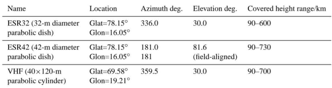
Table 1. Parameters of the EISCAT radars for the experiment on 21 February 2002.
Name Location Azimuth deg. Elevation deg. Covered height range/km ESR32 (32-m diameter Glat=78.15◦ 336.0 30.0 90–600
parabolic dish) Glon=16.05◦
ESR42 (42-m diameter Glat=78.15◦ 181.0 81.6 90–730 parabolic dish) Glon=16.05◦ 181 (field-aligned)
VHF (40×120-m Glat=69.58◦ 359.5 30.0 90–700
parabolic cylinder) Glon=19.21◦
ground-based methods are available. Since the location of such profiles depends only on the LEO satellite path, which eventually covers the whole globe, data can be obtained, for instance, over oceans or over other inaccessible areas. This is very important for global studies, particularly in the context of space weather events. Therefore, it is important to verify occultation profiles with other techniques and to obtain expe-rience in the reliability of their derivation. This study should serve as a step in this direction.
For the incoherent scatter radar (ISR) measurements the EISCAT mainland (UHF and VHF) and EISCAT Svalbard radars (ESR) have been used. The incoherent scatter tech-nique has been described in detail in many publications (e.g. Rishbeth and van Eyken, 1993) and will therefore not be re-peated here. All EISCAT radars have been used with differ-ent antenna pointing directions as described in the following. The post integration of the measurements was of the order of a few minutes, in order to match the time intervals needed to derive an occultation profile. Since novel pulse codes and processing techniques are used in the measurements (Nygr´en et al., 1996), the height range resolution of the profiles was variable, i.e. a few kilometres below 150 km height up to about 35 km in the topside ionosphere. In the ESR and VHF radars the alternating code programmes τ 0 and τ 1 were used and the data from several heights were added together to give a height resolution of approximately 12 km (ESR42), 20 km (ESR32), and 30 km (VHF) in the F region (in ∼300 km al-titude), respectively. For the UHF radar 22.5 km long pulses from the cp1lt modulation were used. It should be noted that a height resolution of the order of 20 km may result in un-derestimating the peak densities of thin layers by about 2% (Sedgemore et al., 1996).
Incoherent scatter radars measure relative electron density profiles very well, but the absolute density needs to be cali-brated by some other means. This is usually done with the help of ionograms, whereby the critical frequencies from the ionogram are used to calibrate the peak density (e.g. Sedge-more et al., 1996). Commonly, calibration is performed for the F2 peak. In practice, the calibration constant sometimes changes and therefore needs to be checked in reasonable time intervals. The EISCAT mainland UHF radar analysed data is regularly calibrated by the use of the Tromsø dynasonde at the EISCAT site. For the 25 and 26 November 2001 data the peak F2 peak densities agreed to within 10%.
The ESR32 radar-derived F2 peak densities have been compared with peak densities from a co-located ionosonde for April and July 1999 (Bempong, 2001), but which was operating only until May 2001. For moderate ionospheric conditions without important irregularities, F2 peak densi-ties obtained with the ESR 32 m antenna were found to be 4% below the ionosonde peak densities. Van Eyken (2001) presented comparisons between ESR32 and mainland UHF, where ESR32 estimated densities on average 4% lower than UHF: however, deviating points of up to 30% occurred. The same presentation includes a comparison between the Sval-bard ionosonde and the ESR42 radar. It was shown that the ESR 42 measured a 12% higher F2 peak density than the ionosonde indicated. Holt and van Eyken (2000) plot-ted electron densities of the ESR32 against VHF and found a good average agreement but with again some deviating points up to 30%. However, at the time of our campaign there was no operating ionosonde on Svalbard for synchronous calibration of ESR. The mainland VHF radar is calibrated to ionograms not very regularly, because the two instruments (VHF and Tromsø dynasonde) mostly observe different vol-umes. Nevertheless, supported by the above mentioned in-vestigations, the accuracy of the ESR32, ESR42 and the mainland VHF are believed to be correct to within 10–20%.
The EISCAT radar facility has been a powerful tool for comparisons with different ionospheric studies using navi-gational signals, especially with tomographic electron den-sity reconstructions (several experiments are published, e.g. in Kersley, 1995). Due to the high cost of running the radar, campaigns are restricted in time. So far, three cam-paigns have been conducted within the SIRCUS program, in November 2001, February 2002 and May/June 2002. We will report results here from all these campaigns.
2 Detailed description example on 21 February 2002
Data obtained on 21 February 2002 will be described here in some detail in order to illustrate the techniques and methods used in all cases.
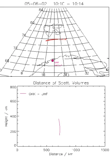
The geometry of the experiments is sketched in Fig. 1. The upper panel shows the projection of the IS radar beams on the ground, as well as the occultation trace projected on the ground in a latitude-longitude graph. In this example the
Fig. 1. Upper panel: Projection of the three radar beams and the occultation trace on the ground in a latitude-longitude graph. Lower panel: Distance between the occultation tangential point and the radar scattering volumes at same altitudes.
occultation trace covers the height range of 140 to 420 km. The settings of the three EISCAT radars are summarized in Table 1.
It should be noted that only the ESR42 measures a “near” altitude profile, because of the high elevation of the beam. In the case of the ESR32 and the VHF radar the profile stretches over a long horizontal range as plotted in Fig. 1. The lower panel of Fig. 1 shows the distance between the occultation tangential points and the radar scattering volumes at the same altitude. It illustrates that the measured data were obtained at locations which may be quite far apart.
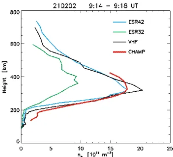
In Fig. 2 we plotted the electron density values versus al-titude measured along the radar beams explained in Fig. 1 together with the electron density profile obtained from the occultation retrieval. Because of the close distances (see Fig. 1) the CHAMP derived profile agrees very well with the VHF and the ESR42 profiles. Large differences in density exist between the occultation profile and the ESR32. These differences are not solely caused by the large distances of around 1150 km, but indicate different ionospheric condi-tions at the measuring sites, as is evident from Fig. 3. It shows the corresponding polar map of the total electron
con-Fig. 2. Electron density values versus altitude measured along the three radar beams, together with the electron density profile ob-tained from the occultation retrieval.
tent (TEC) derived from GPS measurements at numerous ground stations belonging to the global network of the In-ternational GPS Service (IGS) (Jakowski et al., 2002b; see also http://www.kn.nz.dlr.de).
Whereas the occultation trace and the ESR42 and VHF beams are located more or less within the green shaded area, indicating similar electron densities at both sites, the ESR32 beam stretches towards the blue-coloured area, indicating lower electron densities than those near the radar sites. This is in good agreement with the generally lower densities mea-sured along the ESR32 beam.
Since we have evaluated 28 occultations during the three SIRCUS campaigns mentioned above, it is obvious that they cannot all be discussed in this detail. Therefore, we derived certain criteria to summarize the agreement/disagreement of the profiles. This will be the subject of the next section.
3 Summary of all observations
All evaluated occultation events are summarised in Table 2. It contains in the first four columns, date, time, the involved radar, and the local geomagnetic index K of Tromsø. This latter quantity is better suited for judging the local geomag-netic activity than the global Kp index. The fifth column
shows the difference of the height of the F2 peak between the occultation and the corresponding radar profile 1Hp.
This and the following differences of the quantities P are calculated as PIRO–PISR, or in the case of a relative
dif-ference as PIRO–PISR/PISR. The sixth column contains the
difference of the F2 peak density between the occultation and the radar results 1Nep. Since these peak densities vary
be-tween about 2×10¹¹and 2×10¹²m−3for the different cases, a relative difference is more suitable here. The seventh
col-2018 C. Stolle et al.: Comparison of high latitude electron density profiles
Table 2. Summary of all observed 28 occultation events. K is the local geomagnetic index for Tromsø. 1Hp=Hp IRO–Hp ISR,
Nep=(Nep IRO–Nep ISR)/ Nep ISR, Distance=peakIRO–peakISR, 1TEC=(TECIRO(150–420 km) –TECISR(150–420 km)) / TECISR(150–
420 km).
Date Time (UT) Radar K d1Hp(km) 1Nep(%) Distance (km) 1TEC (%)
25 November 2001 17:12 UHF 2 –14 21 560 25 26 November 2001 02:30 UHF 3 –22 –19 275 –31 26 November 2001 16:27 UHF 0 –18 45 566 70 27 November 2001 15:41 UHF 1 –2 –38 1137 –21 17 February 2002 09:25 ESR42 2 –92 2 722 24 17 February 2002 21:51 ESR42 4 –53 –52 1088 –40 19 February 2002 12:27 VHF 1 20 –44 598 –44 19 February 2002 20:16 ESR42 2 –35 76 533 94 20 February 2002 08:48 ESR42 1 83 –57 109 –53 20 February 2002 08:33 VHF 1 45 –71 409 –70 21 February 2002 09:15 ESR42 1 4 1 593 18 21 February 2002 09:15 ESR32 1 –55 91 1120 142 21 February 2002 09:15 VHF 1 –26 –4 350 4 21 February 2002 12:25 ESR42 1 24 25 506 39 21 February 2002 12:25 ESR32 1 –14 10 108 15 21 February 2002 12:25 VHF 1 39 –29 937 –12 22 February 2002 08:28 ESR42 1 –35 –54 609 –54 22 February 2002 08:28 ESR32 1 –202 80 102 136 22 February 2002 08:28 VHF 1 –32 –75 1077 –76 29 May 2002 23:51 UHF 3 –16 1 815 9 30 May 2002 10:45 UHF 2 28 –19 1130 –13 30 May 2002 22:57 UHF 1 8 11 798 –6 31 May 2002 23:40 UHF 1 –16 –26 824 –16 01 June 2002 10:31 UHF 1 –13 –19 997 –17 03 June 2002 10:23 UHF 2 6 –18 857 –13 04 June 2002 00:06 UHF 3 –15 9 1164 –24 04 June 2002 23:18 UHF 3 –37 –11 1120 7 05 June 2002 10:12 UHF 2 11 17 722 8
umn gives the distance between the F2 peaks of the occul-tation and the radar profiles (taken from calculations as dis-played in the lower panel of Fig. 1). Finally, column eight contains a relative difference of the total electron content cor-responding to the occultation and the radar profiles, 1TEC. Note that the total electron content calculated here is differ-ent from the ground-based GPS-determined one which leads to the TEC map (Fig. 3). In order to obtain a comparable
quantity between the occultation and the radar profiles, it was calculated from the measured profiles within the height range 150–420 km, i.e. does not contain the top side iono-sphere and the plasmaiono-sphere, but clearly the F2 peak. In some cases, when the occultation profile did not reach the upper limit of 420 km, it was logarithmically extrapolated. TEC is a quantity which is very important for the correction of GPS positioning and surveying in case of high precision
Fig. 3. TEC obtained using IGS network data over the Northern Hemisphere for times close to the occultation event at 21 February 2002. (1 TECUnit=1×10¹⁶electrons/m2).
requirements. A relative TEC error characterizing the relia-bility of occultation profiles is therefore an important param-eter.
Table 2 provides a convenient way to compare the occulta-tion and radar profiles. The three cases menocculta-tioned in Sect. 2 are represented in lines 11–13 of the table.
4 Discussion
In order to discuss the results summarized in Table 2 we start with three correlation plots of 1Hp, 1Nep, and 1TEC
as a function of the distance of the corresponding F2 peaks (Fig. 4).
For comparing the F2 peak height (upper panel of Fig. 4) it should be realized that the height resolution in the F re-gion is of the order of 25 km for both the occultation and the radar profiles. Thus, a 1Hp of ± 25 km can be regarded as
an error bar of the measurements. This limit is plotted as dashed lines in the figure. More than half of the cases, 57%, are within these limits. For the outliers it should be taken into account that the F2 peak is not always clearly defined, either in EISCAT or in the CHAMP data. This leads to ad-ditional differences (e.g. Fig. 7, discussed below). It is also interesting to note that there is only a very weak correlation of 1Hpand the distance of the peaks (the correlation
coeffi-Fig. 4. Correlation plots of F2 peak height difference, 1Hp,
rela-tive difference of F2 peak densities, 1Nep, and relative difference
of total electron content, 1TEC (compiled for height ranges 150– 420 km) as function of the distance of the corresponding F2 peaks (taken from calculations as displayed in Fig. 1)
.
cient is −0.15, not statistically significant). This means that a large distance does not generally result in a great difference in the peak height. Zonal or meridional density structures are probably much more important (see below). The mean 1Hp
averaged over all 28 cases is −10 km which could indicate a small bias, i.e. a systematic underestimation of the peak height by the occultation method. A greater ensemble has to be studied, however, to ascertain such a bias. A compara-tive study with F2 peak height estimations based on vertical sounding data from mid-latitudes has revealed a slight over-estimation of radio occultation retrievals of 13 km within a cross section diameter of 16◦(Jakowski et al., 2002a).
The correlation between 1Nep and the distance (Fig. 4
middle panel) is again not very pronounced (the correlation coefficient is 0.16, not statistically significant). Here we may assume that the measuring error in the density is of the order of 10–20% for the radar and of the same order for radio oc-cultation retrievals in mid-latitudes within a cross section di-ameter of 16◦(Jakowski et al., 2002a). Similar to the case of 1Hp, 60% of the data points are within an error limit of
2020 C. Stolle et al.: Comparison of high latitude electron density profiles
Fig. 5. Electron density values versus altitude measured along the vertical UHF (Tromsø) radar beam, together with the electron den-sity profile obtained from the occultation measurement.
Fig. 6. Upper panel: Projection of the occultation trace on the ground and the location of the EISCAT UHF radar (Tromsø) in a latitude-longitude graph. Lower panel: Distance between the points of the occultation path and the radar scattering volumes at the same altitude.
Fig. 7. Same as Fig. 2, but for the event on 22 February 2002.
about ±30%. Larger differences can again be attributed to zonal or meridional electron density gradients.
For the 1TEC calculations we have assumed an error limit of about ±40%, taking into account the above considerations concerning its retrieval. Again, most of the data points (64%) are within this error band (Fig. 4, lower panel). The corre-lation coefficient of 1TEC and the peak distance is −0.14, again a value which is not statistically significant.
Larger differences in the occultation and radar profiles may also be expected during disturbed conditions when the auroral and polar ionosphere can be highly structured. In order to check this we have plotted all the cases with K>2 with a different symbol in Fig. 4 (a solid square). These five points do not significantly contribute to the scattering of all data points. This may be due to the fact that the structuring resulting from geomagnetic activity is more pronounced in the E region which is difficult to access with the occultation technique and is not regarded here, since almost all occulta-tion profiles start above the E-layer in our examples.
For the sake of completeness we also document an aver-age occultation event from the May/June 2002 campaign. Figure 5 shows profiles derived on 5 June 2002 around 10:12 UT from occultation technique and from the EISCAT UHF radar (located near Tromsø/Norway, Glat=69.6◦N, Glon=19.23◦E). The corresponding geometry is explained in Fig. 6. The radar profile was derived for a vertical beam di-rection in all the May/June 2002 campaign cases. The differ-ences of both profiles in 1Hp, 1Nep, and 1TEC are within
the error limits indicated in Fig. 4, thus we regard them as not significant. The TEC map of most events of this campaign are fairly uniform and do not indicate much structure in the sunlit ionosphere.
We do not want to conceal that there are a few cases where the occultation and radar profiles look quite different, despite a short distance between both profiles. An example of such
Fig. 8. Same as Fig. 1, but for the event on 22 February 2002.
a case is the event on 22 February 2002 (marked with a little “1” in Fig. 4). As can be seen from Fig. 7, the ESR32-profile does not show a “normal” structure with a pronounced F2 layer but rather a very variable behaviour. The occultation profile shows a single peak at about 300 km height (consid-ered in the analysis as the F2 layer maximum) and an indi-cation of a second peak above. The radio occultation pro-file extends only up to 400 km, but the general propro-file shape also indicates an unusually structured ionosphere. Although the ESR32 beam and the occultation path are almost paral-lel, as displayed in Fig. 8, peaks and valleys of both pro-files are shifted to each other. It should be noted that the ESR32 scattering volume points increase in altitude towards NW, whereas the occultation tangential points decrease in al-titude in this direction. The reason for the structured profile are most probably wave effects (AGW), in conjunction with the sunrise terminator. Since the overall density is quite low at this time, the TEC map (Fig. 9) does not resolve these structures. It can be expected that electron density struc-tures also appear in the horizontal direction within the dis-tances considered here. Furthermore, the fact that the ESR42 and VHF profile structures do not agree with the occultation results in detail, reflects the differences of both measuring methods. Due to the horizontal smoothing of the radio occul-tation technique, local perturbations are in principle not well
Fig. 9. Same as Fig. 3, but for the event on 22 February 2002.
reproduced, in particular if large zonal gradients in electron density appear as revealed by the TEC map (Fig. 9). It also can be taken into account that the ESR32 radar beam and the occultation path look into the night side of the globe and the beams of the ESR42 and the VHF are located in the morning sector.
It is also interesting to note that the occultation technique apparently tends to overestimate the electron density in case of very low densities. Besides the case shown in Fig. 7 we have a few more events with F2 peak densities around 1–2×10¹¹m−3(26 November 2001, 16:27 UT; 19 February 2002, 20:16 UT; 04 June 2002, 00:06 UT) where this effect can be observed. The mentioned comparisons are performed in polar or auroral latitudes. Due to the polar CHAMP or-bit and to the low inclination of 55◦ of the GPS orbits, the occultation rays are mostly north-south directed. Then parts of the occultation rays cross mid-latitude or subtropical re-gions, generally indicating higher ionization. When the polar electron densities are very small the influence of the south-ward ray section will contribute more to the profiling result than it would do for more elevated values at the occultation point. Nevertheless, this is something which will be subject to further studies. A slight overestimation of the F2 layer peak density by radio occultation retrievals has also been found by validation studies for mid-latitudes (Jakowski et al., 2002a) and by comparisons with ionosonde data for auroral latitudes (Stolle et al., 2002).
2022 C. Stolle et al.: Comparison of high latitude electron density profiles
5 Summary and conclusions
We have compared electron density profiles derived from ra-dio occultation measurements on-board CHAMP and from EISCAT incoherent scatter. Similar studies have been pub-lished before (e.g. Hajj and Romans, 1998). This study un-derlines the need of geometric information on the experi-ments of the different profile paths and the use of TEC maps, in order to obtain information about large-scale density struc-tures. Furthermore, we derived quantitative parameters to characterize the differences of the compared profiles: the peak height difference, the relative peak density difference and a relative TEC difference. Most of the compared profiles agree within error limits, depending on the accuracy of the occultation- and the radar-derived profiles. Generally speak-ing, these results agree quite well with validation studies based on a comparison with F2 layer peak density and height data from mid-latitudes (Jakowski et al., 2002a). Greater dif-ferences do not primarily depend on the regional distance between the occultation point and the radar beam but can be attributed to ionospheric zonal and meridonal small- and large-scale structures, which are enhanced, for example, dur-ing dawn and dusk and perturbed geomagnetic conditions.
Acknowledgements. The authors thank the EISCAT Director and staff for running the radar and providing the data. EISCAT is a sci-entific association of national funding agencies of France, Finland, Germany, Japan, Norway, Sweden and the United Kingdom. We are grateful to the colleagues at the GeoForschungsZentrum Potsdam, DLR and JPL involved in the CHAMP mission to keep the satellite in operation and to provide corresponding data services.
Topical Editor M. Lester thanks C. Mitchell and another referee for their help in evaluating this paper.
References
Bempong, C. N.: F-region electron densities above Svalbard: A comparison between incoherent scatter and ionosonde methods, M. Phil. Thesis, University of Tromso, 2001.
Hajj, G. A. and Romans, L. J.: Ionospheric electron density profiles obtained with the Global Positioning System: Results from the GPS/MET experiment, Radio Sci., 33, 175–190, 1998.
Holt, J. M. and van Eyken, A. P.: Plasma convection at high lati-tudes using the EISCAT VHF and ESR incoherent scatter radars, Ann. Geophys.,18, 1088–1096, 2000.
Jakowski, N., Wehrenpfennig, A., Heise, S., Reigber, Ch., L¨uhr, H., Grunwaldt, L. and Meehan, T.: GPS Radio Occultation Measure-ments of the Ionosphere from CHAMP: Early Results, Geophys. Research Lett., 29 (10), doi:10.1029/2001GL014364, 2002a. Jakowski, N., Heise, S., Wehrenpfennig, A, Schl¨uter, S., and
Reimer: R., GPS/GLONASS-based TEC measurements as a contributor for space weather forecast, J. Atmos. Solar-Terr. Phys.64, 729–735, 2002b.
Kersley, L.: Special Issue: Ionospheric tomography, Ann. Geo-phys., 13(12), 1241–1330, 1995.
Nygr´en, T., Huuskonen, A., and Pollari, P.: Alternating-coded mul-tipulse codes for incoherent scatter experiments, J. Atmos. Terr. Phys., 58, 465–477, 1996.
Rishbeth, H. and van Eyken, A. P.: EISCAT: early history and the first ten years of operation, J. Atmos. Terr. Phys., 55, 525–542, 1993.
Schreiner, W. S., Sokolovskiy, S. V., and Rocken, C.: Analysis and validation of GPS/MET radio occultation data in the ionosphere, Radio Sci., 34, 949–966, 1999.
Sedgemore, K. J. F., Williams, P. J. S., Jones, G. O. L., and Wright, J. W.: A comparison of EISCAT and dynasonde measurements of the auroral ionosphere, Ann. Geophys., 14, 1403–1412, 1996. Stolle, C., Lange, M. and Jacobi, Ch.: Validation of atmospheric temperature profiles and electron densities derived from CHAMP radio occultation measurements during measurement campaigns at Andoya (69.28◦N, 16.02◦E), Rep. Inst. Meteorol. Univ. Leipzig , 2002.
van Eyken, A. P.: Sanity Checks and other calibrations, paper presented at the 10th International EISCAT Workshop, Tokyo, Japan, 2001.