HAL Id: hal-00709946
https://hal.archives-ouvertes.fr/hal-00709946
Submitted on 7 Aug 2020
HAL is a multi-disciplinary open access
archive for the deposit and dissemination of
sci-entific research documents, whether they are
pub-lished or not. The documents may come from
teaching and research institutions in France or
abroad, or from public or private research centers.
L’archive ouverte pluridisciplinaire HAL, est
destinée au dépôt et à la diffusion de documents
scientifiques de niveau recherche, publiés ou non,
émanant des établissements d’enseignement et de
recherche français ou étrangers, des laboratoires
publics ou privés.
Marion Kersale, Andrea Doglioli, Anne Petrenko
To cite this version:
Marion Kersale, Andrea Doglioli, Anne Petrenko. Sensitivity study of the generation of mesoscale
eddies in a numerical model of Hawaii islands. Ocean Science, European Geosciences Union, 2011, 7,
pp.277-291. �10.5194/os-7-277-2011�. �hal-00709946�
www.ocean-sci.net/7/277/2011/ doi:10.5194/os-7-277-2011
© Author(s) 2011. CC Attribution 3.0 License.
Ocean Science
Sensitivity study of the generation of mesoscale eddies in a
numerical model of Hawaii islands
M. Kersalé, A. M. Doglioli, and A. A. Petrenko
Aix-Marseille Université, CNRS, IRD, LOPB-UMR 6535, Laboratoire d’Océanographie Physique et Biogéochimique, OSU/Centre d’Océanologie de Marseille, France
Received: 8 February 2010 – Published in Ocean Sci. Discuss.: 10 March 2010 Revised: 9 April 2011 – Accepted: 13 April 2011 – Published: 2 May 2011
Abstract. The oceanic circulation around the Hawaiian archipelago is characterized by a complex circulation and the presence of mesoscale eddies west of the islands. These ed-dies typically develop and persist for weeks to several months in the area during persistent trade winds conditions. A series of numerical simulations on the Hawaiian region has been done in order to examine the relative importance of wind, inflow current and topographic forcing on the general cir-culation and the generation of eddies. Moreover, numerical cyclonic eddies are compared with the one observed during the cruise E-FLUX (Dickey et al., 2008). Our study demon-strates the need for all three forcings (wind, inflow current and topography) to reproduce the known oceanic circulation. In particular, the cumulative effect plays a key role on the generation of mesoscale eddies. The wind-stress-curl, via the Ekman pumping mechanism, has also been identified as an important mechanism upon the strength of the upwelling in the lee of the Big Island of Hawaii. In order to find the best setup of a regional ocean model, we compare more pre-cisely numerical results obtained using two different wind databases: COADS and QuikSCAT. The main features of the ocean circulation in the area are well reproduced by our model forced by both COADS and QuickSCAT climatolo-gies. Nevertheless, significant differences appear in the lev-els of kinetic energy and vorticity. The wind-forcing spatial resolution clearly affects the way in which the wind momen-tum feeds the mesoscale phenomena. The higher the resolu-tion, the more realistic the ocean circulation. In particular, the simulation forced by QuikSCAT wind data reproduces well the observed energetic mesoscale structures and their hydrological characteristics and behaviors.
Correspondence to: M. Kersalé
1 Introduction
The oceanic area around the Hawaiian archipelago exhibits a complex circulation characterized by the presence of mesoscale eddies west of the islands. This circulation is mainly due to the effects of the archipelago topographic forc-ing on both the North Equatorial Current (NEC) and the trade wind. Indeed, the blocking effect of the Hawaiian islands bathymetry on the oceanic flow is similar to the one of these islands’ topography on the wind.
The NEC is a broad westward flow, constituting the south-ern part of the North Pacific subtropical gyre. When the NEC encounters the island of Hawaii, it is deflected towards the south, but also generates a northern branch (Lumpkin, 1998). The northern branch is known as the North Hawaiian Ridge Current (NHRC), flowing coherently along the islands at an average speed of 0.10–0.15 m s−1 (Qiu et al., 1997). The wake generated by the Hawaiian island is thought respon-sible for the formation of the Hawaiian Lee Counter Current (HLCC).
By a classical mechanism of formation of eddies in the lee of an obstacle, the wake can also generate mesoscale ed-dies, as indicated by the observations reported downstream of Gran Canaria Island (Aristegui et al., 1994, 1997; Bar-ton et al., 2000). In the case of Hawaii, south (north) of the HLCC these eddies are typically anticyclonic (cyclonic) (Lumpkin, 1998).
A second mechanism could also explain the formation of an important counter-current (here the HLCC) and mesoscale eddies (whether in Hawaii or Gran Canaria). Lumpkin (1998) showed that there is an eddy-to-mean kinetic energy conversion at the latitude of the HLCC immediately west of the Island of Hawaii. By a simple Sverdrup balance, Cha-vanne et al. (2002) predict an HLCC from the wind stress curl dipole in the lee of the island of Hawaii. As explained
islands act as barriers to the trade winds, which are confined below the tropopause and constrained to flow around the to-pography (Chavanne et al., 2002). The wind stress variations in the lee of the Hawaiian Islands drive divergent and conver-gent Ekman transports in the upper layer of the ocean. And, in particular, the acceleration of the persistent northeasterly trade winds through the Alenuihaha Channel separating these islands is the second mechanism generating mesoscale ed-dies (Patzert, 1969). West of the islands, this mechanism can create cyclonic eddies south of 20◦N and anticyclonic eddies north of 20◦N.
Historical hydrographic and satellite data sets (Patzert, 1969; Lumpkin, 1998; Chavanne et al., 2002; Seki et al., 2001, 2002; Bidigare et al., 2003) indicate that mesoscale eddies typically develop and persist for weeks to several months west of the Hawaiian archipelago during persistent trade wind conditions. Moreover, interdisciplinary observa-tions of mesoscale eddies were recently made west of the Big Island of Hawaii, combining different data from ships, surface drifters and satellite sensors (Dickey et al., 2008, project E-FLUX). During the cruises E-FLUX I and III, two cold-core cyclonic mesoscale eddies, Noah and Opal, respec-tively, have been found.
To simulate the oceanic circulation around the Hawai-ian islands, we used a version of the model ROMS (Re-gional Oceanic Modeling System) provided with the follow-ing ROMSTOOLS (http://roms.mpl.ird.fr). This modelfollow-ing system is increasingly used, since its functionality and ro-bustness have been demonstrated. Different physical straints can be implemented with regard to boundary con-ditions and bottom stress. Different databases can also be used to provide atmospheric forcing to ROMS model, such as COADS (Comprehensive Ocean-Atmosphere Data Set Project) and data collected by NASA’s SeaWinds Scatterom-eter aboard QuikSCAT.
Dong and McWilliams (2007) used the model ROMS to study vortex shedding by deep water islands and topographic eddy forcing in the Southern California Bight. Yoshida et al. (2010) studied the wind forcing of Hawaiian eddies. They found that, in the immediate lee southwest of Hawaii (18.9◦N–20◦N, 158◦W–156.7◦W), eddy signals have a pre-dominant 60-day period and a short life-span. They noticed that the observed eddies originate in the southwest corner of Hawaii and are induced by the local wind stress curl vari-ability associated with the blocking of the trade winds by the island of Hawaii. Jiménez et al. (2008) performed several experiments to study the relative importance of topographic and wind forcing on oceanic eddy shedding by an isolated, tall, deep water island. They applied the model to the case of eddies shed by the island of Gran Canaria. They found that wind forcing alone is not sufficient to force an oceanic Von Karman vortex street in the lee of the island and that topo-graphic forcing is necessary. In their case, the wind forcing
current alone is not sufficiently energetic to produce vortex shedding.
As regards wind forcing, monthly mean values from COADS were compared to monthly mean wind speed and di-rection from Canadian weather buoys in the northeast Pacific (Cherniawsky and Crawford, 1996). Wind speed measure-ments from QuikSCAT scatterometer were validated by parison with independent data. For instance, they were com-pared with meteorological analyses (Renfrew et al., 2009) over the Denmark Strait, or with wind speeds computed from RADARSAT-1 synthetic aperture radar (SAR) in the Gulf of Alaska (Monaldo et al., 2004). Concerning ocean model-ing, the influence of COADS versus QuickSCAT wind data on oceanic circulation was analyzed in the California Cur-rent System (Penven et al., 2002). Calil et al. (2008) have done numerical modeling simulations of the ocean response to realistic wind forcing in the lee of the Hawaiian Island chain. Since we use the same methodology, we stress, in this paper, the similarities and differences between their and our results. On the North equatorial central Pacific, an ocean model forced by COADS wind versus one forced by the NCEP-NCAR (National Centers for Environmental Predic-tion – NaPredic-tional Center for Atmospheric Research) reanalysis wind were used to compare the observations of ocean heat content (Wu and Xie, 2003). Independent observations of oceanic circulation were investigated with an ocean model forced by QuikSCAT wind data in different regions: the Pa-cific system (Xie et al., 2001) and the Southern Benguela upwelling system (Blanke et al., 2005).
The main purpose of this study is to analyze the relative importance of topography and wind forcing on the Hawaiian oceanic circulation and eddies generation, with particular at-tention to wind-driven mesoscale eddy generation simulated with both COADS and QuikSCAT wind data.
The paper is organized as follows: Sect. 2 introduces briefly the numerical model, the main simulation and eddy tracking parameters. Section 3 presents the model sensitiv-ity and a discussion about the variabilsensitiv-ity in the surface wind stress. This part will allow us to analyze whether the model reproduces the generation of mesoscale eddies west of the Hawaiian archipelago. In Sect. 4, we analyze which simula-tion is the more realistic and whether one forcing is predom-inant. Our conclusions are drawn in Sect. 6.
2 Materials and methods 2.1 Ocean Model
Our circulation model is based on the IRD (Institut de Recherche pour le Développement) version of the Regional Ocean Modeling System (ROMS). The reader is referred to Shchepetkin and McWilliams (2003, 2005) for a more
161oW 160oW 159oW 158oW 157oW 156oW 155oW 154oW 18oN 19oN 20oN 21oN 22oN 23oN BIG ISLAND MAUI MOLOKAI OAHU KAUAI Alenhuihaha Channel 500 1000 1500 2000 2500 3000 3500 4000 4500 5000
Fig. 1. Model domain and bathymetry [m]. Names of the islands
and coastline at higher resolution are reported for geographical in-formation.
complete description of the numerical code. The model do-main extends from 154◦W to 161◦W and from 18◦N to 23◦N (Fig. 1).
Its grid, forcing, initial and boundary conditions were built with the ROMSTOOLS package (Penven et al., 2010). The model grid is 69 × 53 points with a resolution of 101◦ corre-sponding to about 10 km in mean grid spacing, which allows a correct sampling of the first baroclinic Rossby radius of deformation throughout the whole area (about 60 km accord-ing to Chelton et al., 1998). The horizontal grid is isotropic with no introduction of asymmetry in the horizontal dissi-pation of turbulence. It therefore provides a fair represen-tation of mesoscale dynamics. The model has 32 vertical levels, and the vertical s-coordinate is stretched for bound-ary layer resolution. The bottom topography is derived from a 20 resolution database (Smith and Sandwell, 1997). Al-though a numerical scheme associated with a specific equa-tion of state limits errors in the computaequa-tion of the horizontal pressure gradient (Shchepetkin and McWilliams, 2003), the bathymetry field, h, must be filtered to keep the slope param-eter, r, as r =|∇h|2h ≤0.25 (Beckmann and Haidvogel, 1993). Respecting the CFL criterion, the external (internal) timestep has been fixed equal to 12 s (720 s).
At the four lateral boundaries facing the open ocean, the model solution is connected to the surroundings by an active, implicit and upstream-biased radiation condition (Marchesiello et al., 2001). Under inflow conditions, the solution at the boundary is nudged toward temperature-, salinity- and geostrophic velocity-fields calculated from Lev-itus 1998 climatology (NODCWOA98 data provided by the NOAA/OAR/ESRL PSD, Boulder, Colorado, USA, from their Web site at http://www.cdc.noaa.gov/), which is also used for the initial state of the model. The nudging timescale for inflow and outflow (τin, τout) are set to (1 day, 1 yr) for the
tracer fields and (10 days, 1 yr) for the momentum fields. The
Table 1. Summary of the performed numerical experiments, the
relatives names and the forcings.
Name Wind forcing Advection Drag Coeff. Run-A none Ugeo Cd
Run-B none 2Ugeo Cd
Run-C QuikSCAT none Cd
Run-D QuikSCAT Ugeo none
Run-E COADS Ugeo Cd
Run-F QuikSCAT Ugeo Cd
geostrophic velocity (Ugeo) is referenced to the 2000 m level.
The width of the nudging border is 100 km, and the maxi-mum viscosity value for the sponge layer is set to 800 m2s−1. Bottom boundary conditions for momentum are computed by assuming a logarithmic velocity profile and using a bot-tom roughness (Zob=1.10−2m) to determine a quadratic
drag coefficient for a typical stress boundary condition of τb=Cdρou|u| where τbis the bottom frictional stress, ρ0the
water density, Cdthe drag coefficient and u the bottom
cur-rent. The drag coefficient is defined as Cd=ln(z/Zk
ob) ranging
from a minimum of 10−4and a maximum of 10−1coefficient with k the Von Karman constant.
At the surface, the heat and fresh water fluxes introduced in the model are extracted from the Comprehensive Ocean-Atmosphere Data Set (COADS, Da Silva et al., 1994). As regards wind stress, two different databases are used in this work: (i) a monthly mean climatology computed from COADS dataset (1945–1989) giving data with spatial resolu-tion of 12◦; (ii) a monthly mean climatology computed from satellite-based QuikSCAT dataset (2000–2007, Callahan and Lungu, 2006) gridded at 14◦resolution.
Table 1 summarizes the performed numerical experiments. In all cases, we run 10-yr simulations with model outputs averaged and stored every 3 days of simulation.
The two first experiments (Run-A and Run-B) are made with no wind forcing and different values for the inflow ve-locities at the open boundary. In the third experiment (Run-C), the inflow velocity is set to zero and the wind forcing comes from the QuikSCAT database. In Run-D, the drag co-efficient is set equal to zero. The two last experiments, with both advection and bottom friction, allow to compare the ef-fect of different wind forcing dataset: COADS (Run-E) and QuikSCAT (Run-F).
2.2 Eddy tracking and characterization
To detect eddies, we select a threshold value of the sea sur-face height (ssh) of |5| cm. We choose to set this value to one third of the typical ssh anomaly generated by anticyclonic ed-dies in the Hawaii region (i.e. 15 cm, according to Firing and Merrifield, 2004). Each cyclone (anticyclone) is then listed by the letter C (A) followed by the number corresponding to
280 M. Kersalé et al.: Sensitivity study of the generation of Hawaii mesoscale eddies 0 1 2 3 4 5 6 7 8 9 10 0 10 20 30 40
Volume averaged kinetic energy [cm2.s−2]
0 1 2 3 4 5 6 7 8 9 10 0 200 400 600 800
Surface averaged kinetic energy [cm(a) Run-A 2.s−2]
0 1 2 3 4 5 6 7 8 9 10 0 10 20 30 40
Volume averaged kinetic energy [cm2.s−2]
0 1 2 3 4 5 6 7 8 9 10 0 200 400 600 800
Surface averaged kinetic energy [cm(b) Run-B 2.s−2]
0 1 2 3 4 5 6 7 8 9 10 0 10 20 30 40
Volume averaged kinetic energy [cm2.s−2]
0 1 2 3 4 5 6 7 8 9 10 0 200 400 600 800
Surface averaged kinetic energy [cm(c) Run-C 2.s−2]
0 1 2 3 4 5 6 7 8 9 10 0 10 20 30 40
Volume averaged kinetic energy [cm2.s−2]
0 1 2 3 4 5 6 7 8 9 10 0 200 400 600 800
Surface averaged kinetic energy [cm(d) Run-D 2.s−2]
0 1 2 3 4 5 6 7 8 9 10 0 10 20 30 40
Volume averaged kinetic energy [cm2.s−2]
0 1 2 3 4 5 6 7 8 9 10 0 200 400 600 800
Surface averaged kinetic energy [cm(e) Run-E 2.s−2]
0 1 2 3 4 5 6 7 8 9 10 0 10 20 30 40
Volume averaged kinetic energy [cm2.s−2]
0 1 2 3 4 5 6 7 8 9 10 0 200 400 600 800
Surface averaged kinetic energy [cm(f) Run-F 2.s−2]
Fig. 2. Temporal evolutions (model time, years) of volume-averaged kinetic energy [cm2s−2
] for the six numerical experiments. The horizontal lines indicate the 10-year mean values.
Fig. 2. Temporal evolutions (model time, years) of volume-averaged kinetic energy [cm2s−2] for the six numerical experiments. The horizontal lines indicate the 10-yr mean values.
their temporal appearance. To indicate in which experiment eddies are observed, a letter listing the Run is added at the end of each name of the eddy.
In the following we focus on numerical cyclones chosen because they are spatially and temporally representative of cyclone Opal studied during the cruise E-FLUX III (10–28 March 2005) and observed on SST satellite images from February to April of that year (Nencioli et al., 2008). The characteristics used to chose numerical cyclones resembling the most Opal are the following: generation date, position and life-time. We propose a quantitative comparison between the numerical eddies and Opal based on eddy characteristics’ statistics during the last five years of simulation. Moreover we illustrated this comparison with figures issued from the tenth year of simulation.
Following Dickey et al. (2008), we define the radial ex-tent of the eddy as the distance between the locations where isopycnal and isotherm surfaces become nearly horizon-tal. Indeed, according to these authors, the σt24 (i.e. σt=
24 kg m−3) isopycnal surface proved to be an important
ref-erence in determining the general characteristics of cyclones in this area. Moreover, we calculate the east-west (north-south) components of the horizontal velocity vector along a north-south (east-west) transect for the most realistic numer-ical eddy. In this way we can both (i) estimate the position of the eddy center, as the location where the components of the horizontal velocity are very small and (ii) calculate the eddy radius, as the maximum distance until which, starting at the center, the intensity of the barotropic velocity increases
lin-early (corresponding to the solid body rotation, e.g. Nencioli et al., 2008). This latter distance allows us to also check the previous evaluation of the eddy extent.
3 Results
3.1 Kinetic energy
The temporal evolutions of the volume-averaged kinetic en-ergy for all simulations are reported in Fig. 2. The Run-A results are characterized by the lowest kinetic energy and smallest temporal variability. When the speed of the cur-rents at the boundary is more intense (Run-B), the 10-yr mean value of volume-averaged kinetic energy goes from 22 to 27 cm2s−2. This mean value is of the same or-der than the one of the Run-C result (28 cm2s−2) but the temporal variability of Run-C is higher than the one of Run-B. The Run-D results are characterized by the high-est kinetic energy (32 cm2s−2) and largest temporal
vari-ability. The Run-F results are generally more energetic (30 cm2s−2) than the Run-E ones (27 cm2s−2). Moreover, the kinetic energy has a lower temporal variability in Run-E than in Run-F. We can classify these simulations, from the less to the more energetic with reference to the 10-yr mean value of volume-averaged kinetic energy: Run-A (22 cm2s−2) < Run-B = Run-E (27 cm2s−2) < Run-C (28 cm2s−2) < Run-F (30 cm2s−2) < Run-D (32 cm2s−2).
M. Kersalé et al.: Sensitivity study of the generation of Hawaii mesoscale eddies 281 161oW 160oW 159oW 158oW 157oW 156oW 155oW 154oW 18oN 19oN 20oN 21oN 22oN 23oN 0.3 m s−1 (a) Run-A 161oW 160oW 159oW 158oW 157oW 156oW 155oW 154oW 18oN 19oN 20oN 21oN 22oN 23oN 0.3 m s−1 (b) Run-B 161oW 160oW 159oW 158oW 157oW 156oW 155oW 154oW 18oN 19oN 20oN 21oN 22oN 23oN 0.3 m s−1 (c) Run-C 161oW 160oW 159oW 158oW 157oW 156oW 155oW 154oW 18oN 19oN 20oN 21oN 22oN 23oN 0.3 m s−1 (d) Run-D 161oW 160oW 159oW 158oW 157oW 156oW 155oW 154oW 18oN 19oN 20oN 21oN 22oN 23oN 0.3 m s−1 (e) Run-E 161oW 160oW 159oW 158oW 157oW 156oW 155oW 154oW 18oN 19oN 20oN 21oN 22oN 23oN 0.3 m s−1 (f) Run-F
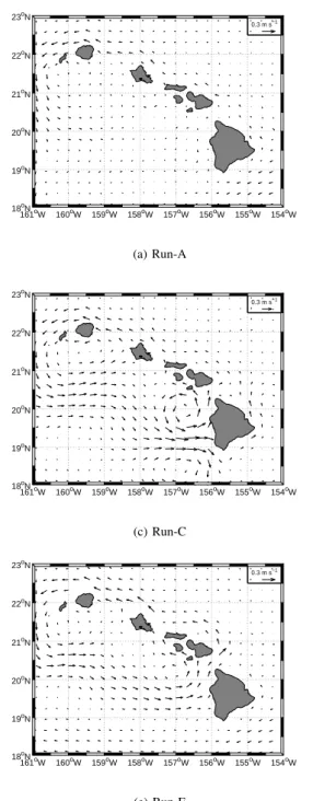
Fig. 3. Annually-averaged currents’ velocity vectors at 40-m depth. Fig. 3. Annually-averaged currents’ velocity vectors at 40-m depth.
3.2 Topographic forcing with advection and no wind
In this experiment, the objective is to analyze the importance of the topographic forcing on the Hawaiian oceanic circula-tion. With this aim in view, wind forcing is suppressed and the intensity of the inflow velocity is set to Ugeo in Run-A
and has been doubled (2Ugeo) in Run-B. In general, the
an-nually averaged circulation of Run-A does not reproduce the NEC and the HLCC (Fig. 3a). In the Run-B (Fig. 3b) the NEC split is well reproduced. To study the mesoscale
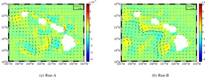
struc-tures, the situation on 22 August is presented in both Run-A and Run-B (Fig. 4). Mesoscale structures dominate the flow field with cyclonic and anticyclonic eddies present in the two simulations. The vortex shedding leads to the formation of a street of successive cyclonic and anticyclonic eddies, look-ing like a Karman vortex street, downstream the Big Island. The numerical results show that the formation of cyclonic eddies frequently occurs on the lee side of other islands, as indicated by the observations reported downstream of Lanai
282 M. Kersalé et al.: Sensitivity study of the generation of Hawaii mesoscale eddies 14 Kersalé et al.: Sensitivity study of the generation of Hawaii mesoscale eddies
161oW 160oW 159oW 158oW 157oW 156oW 155oW 154oW 18oN 19oN 20oN 21oN 22oN 23oN 0.3 m s−1 −4 −3 −2 −1 0 1 2 3 4 x 10⁻⁵ (a) Run-A 161oW 160oW 159oW 158oW 157oW 156oW 155oW 154oW 18oN 19oN 20oN 21oN 22oN 23oN 0.3 m s−1 −4 −3 −2 −1 0 1 2 3 4 x 10⁻⁵ (b) Run-B
Fig. 4. Relative vorticity field with velocity vectors at 10-m depth on August 22 for Run-A (left) and Run-B (right).
161oW 160oW 159oW 158oW 157oW 156oW 155oW 154oW 18oN 19oN 20oN 21oN 22oN 23oN 0.06 0.065 0.07 0.075 0.08 0.085 0.09 (a) COADS 161oW 160oW 159oW 158oW 157oW 156oW 155oW 154oW 18oN 19oN 20oN 21oN 22oN 23oN 0.06 0.07 0.08 0.09 0.1 0.11 0.12 0.13 0.14 (b) QSCAT
Fig. 5. Annually-averaged wind stress values [Nm−2]. Different scales are used for a better visualization.
Fig. 4. Relative vorticity field with velocity vectors at 10-m depth on 22 August for Run-A (left) and Run-B (right). 161oW 160oW 159oW 158oW 157oW 156oW 155oW 154oW 18oN 19oN 20oN 21oN 22oN 23oN 0.3 m s−1 −4 −3 −2 −1 0 1 2 3 4 x 10⁻⁵ (a) Run-A 161oW 160oW 159oW 158oW 157oW 156oW 155oW 154oW 18oN 19oN 20oN 21oN 22oN 23oN 0.3 m s−1 −4 −3 −2 −1 0 1 2 3 4 x 10⁻⁵ (b) Run-B
Fig. 4. Relative vorticity field with velocity vectors at 10-m depth on August 22 for Run-A (left) and Run-B (right).
161oW 160oW 159oW 158oW 157oW 156oW 155oW 154oW 18oN 19oN 20oN 21oN 22oN 23oN 0.06 0.065 0.07 0.075 0.08 0.085 0.09 (a) COADS 161oW 160oW 159oW 158oW 157oW 156oW 155oW 154oW 18oN 19oN 20oN 21oN 22oN 23oN 0.06 0.07 0.08 0.09 0.1 0.11 0.12 0.13 0.14 (b) QSCAT
Fig. 5. Annually-averaged wind stress values [Nm−2]. Different scales are used for a better visualization.
Fig. 5. Annually-averaged wind stress values [Nm−2]. Different scales are used for a better visualization.
Island (Dong et al., 2009). In Run-A, anticyclones tend to dominate south of 19–20◦N and cyclones to be more present in the north. In Run-B, a current is accelerated through the Alenuihaha Channel, inducing vorticity (Fig. 4b). This is not observed in Run-A. This contribution of vorticity induces the formation of anticyclonic eddies between two cyclones re-gions. If we compare the two simulations, the structures from Run-B are more coherent and intense than the ones from Run-A. In Run-B, the vortex shedding frequency increases in time with increasing velocity current. We can calculate the Strouhal number St =D/TU defining the eddy shed-ding frequency, where D is the diameter of the Big Island (100 km), T the shedding period and U the current speed. The period for eddy shedding is roughly 60 days (30 days) for Run-A (Run-B). The mean value of the current speed at 10-m depth is equal to 0.011 m s−1(Run-A) and 0.033 m s−1 (Run-B). This values give Stapproximately equal to 1.75 for Run-A and 1.17 for Run-B. These values are representative of a non-stationary flow where eddies are generated
period-ically downstream the obstacle. For experiments in a ho-mogeneous, non rotating flow, St=0.2 (Zdravkovich, 1997). This implies that eddies are shed at a lower frequency in these experiments.
3.3 Wind forcing comparison
A unidirectional wind regime, stemming from the north-east (i.e. trade winds), is predominant in both datasets (data not shown). As foreseen, the annually averaged values of the two wind stress datasets have significant differences (Fig. 5). In COADS, the prevailing wind stress intensity is in the range 0.06–0.08 Nm2; while, in QuikSCAT, the values are much more intense and the prevailing range is 0.10–0.12 Nm2 (dif-ferent scales are used in Fig. 5 for a better visualization). Strong differences are observed west of all the island chan-nels, including the Alenuihaha Channel, and also south of the Big Island. COADS forcing, due to its resolution, sees the Hawaiian islands as if the archipelago was continuous and contained only one long and distorted island. Hence the
M. Kersalé et al.: Sensitivity study of the generation of Hawaii mesoscale eddies 283 Kersalé et al.: Sensitivity study of the generation of Hawaii mesoscale eddies 15
161oW 160oW 159oW 158oW 157oW 156oW 155oW 154oW 18oN 19oN 20oN 21oN 22oN 23oN 0.3 m s−1 −4 −3 −2 −1 0 1 2 3 4 x 10⁻⁵ (a) April 19 161oW 160oW 159oW 158oW 157oW 156oW 155oW 154oW 18oN 19oN 20oN 21oN 22oN 23oN 0.3 m s−1 −4 −3 −2 −1 0 1 2 3 4 x 10⁻⁵ (b) April 22 161oW 160oW 159oW 158oW 157oW 156oW 155oW 154oW 18oN 19oN 20oN 21oN 22oN 23oN 0.3 m s−1 −4 −3 −2 −1 0 1 2 3 4 x 10⁻⁵ (c) April 25 161oW 160oW 159oW 158oW 157oW 156oW 155oW 154oW 18oN 19oN 20oN 21oN 22oN 23oN 0.3 m s−1 −4 −3 −2 −1 0 1 2 3 4 x 10⁻⁵ (d) April 28
Fig. 6. Relative vorticity field and velocity vectors for Run-C at 10-m depth at different dates in April.
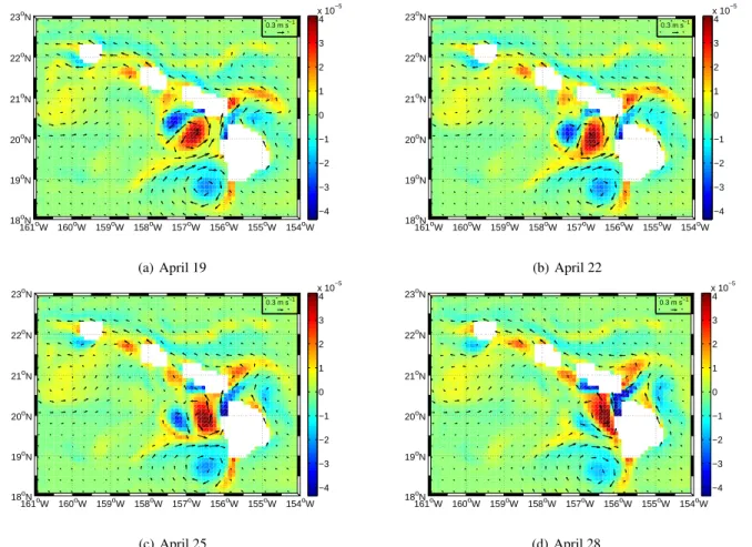
Fig. 6. Relative vorticity field and velocity vectors for Run-C at 10-m depth at different dates in April.
wind stress only accelerates north and south of this unique island. While QuikSCAT forcing captures the effect of each island individually, with an acceleration of the wind stress through the different channels.
3.4 Topographic forcing with QuikSCAT wind forcing and no advection
In this experiment, the objective is to analyze the importance of the wind forcing on the Hawaiian oceanic circulation. In sake of simplicity, we take into account only the wind forcing with the highest resolution: QuikSCAT. The annually aver-aged circulation of Run-C (Fig. 3c) does not show the pres-ence of the NEC. However there is a current similar to the HLCC at 20.5◦N moving progressively towards the south in the lee of the Big Island of Hawaii just between a cyclonic eddy to the north and an anticyclonic one to the south. Circu-lation in April represents well the behavior of the mesoscale structures (Fig. 6). No vortex shedding is produced in this case. But this circulation is dominated by the presence of two eddies, of opposite vorticity, in the Big Island wake: a cyclonic eddy at the exit of the Alenuihaha Channel, centered at 20◦N, and an anticyclonic eddy south of the Big Island of
Hawaii, centered at 18.6◦N. These eddies are intense, with rotational speeds up to 0.4 m s−1, and are stationary all year round. Moreover, we can observe the presence of an anti-cyclonic eddy present northwest of the Alenuihaha anti-cyclonic eddy at the beginning of its life (Fig. 6a). This eddy is gen-erated periodically, every 30 to 60 days. It is characterized by a short life-span (10 days). This eddy circles westward around the Alenuihaha cyclonic eddy, moving progressively towards the south (Fig. 6b, c), and disappears 10 days after its generation (Fig. 6d).
3.5 QuikSCAT wind forcing with advection and no drag coefficient
In this experiment, the model is forced by the inflow veloc-ity at the eastern open boundary (Ugeo) and QuikSCAT wind
forcing, but the drag coefficient is set equal to zero. Look-ing at the annually averaged circulation of Run-D (Fig. 3d), we can note the presence of the NEC in the south and of the HLCC at 19.5–20.5◦N. This circulation is characteristic of a circulation in the lee of an archipelago, forming two dis-tinctive zonal areas (north and south of 20◦N). The HLCC seems to correspond to the border between cyclonic eddies
284 M. Kersalé et al.: Sensitivity study of the generation of Hawaii mesoscale eddies 161oW 160oW 159oW 158oW 157oW 156oW 155oW 154oW 18oN 19oN 20oN 21oN 22oN 23oN 0.3 m s−1 −4 −3 −2 −1 0 1 2 3 4 x 10⁻⁵ (a) April 25 161oW 160oW 159oW 158oW 157oW 156oW 155oW 154oW 18oN 19oN 20oN 21oN 22oN 23oN 0.3 m s−1 −4 −3 −2 −1 0 1 2 3 4 x 10⁻⁵ (b) August 4
Fig. 7. Relative vorticity field and velocity vectors at 10-m depth on April 25 (left) and August 4 (right) for Run-D.
161oW 160oW 159oW 158oW 157oW 156oW 155oW 154oW 18oN 19oN 20oN 21oN 22oN 23oN 0.3 m s−1 −4 −3 −2 −1 0 1 2 3 4 x 10⁻⁵ (a) Run-E 161oW 160oW 159oW 158oW 157oW 156oW 155oW 154oW 18oN 19oN 20oN 21oN 22oN 23oN 0.3 m s−1 −4 −3 −2 −1 0 1 2 3 4 x 10⁻⁵ (b) Run-F
Fig. 8. Relative vorticity field with velocity vectors at 10-m depth on August 25 for Run-E (left) and Run-F (right).
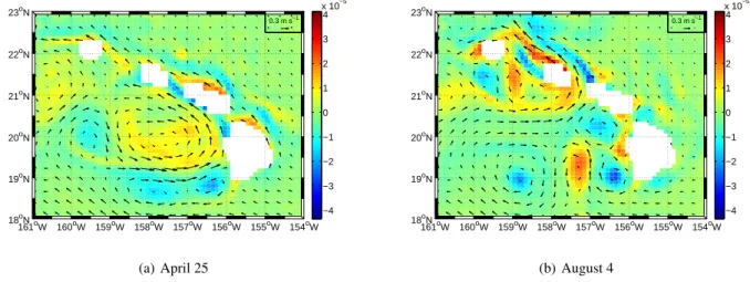
Fig. 7. Relative vorticity field and velocity vectors at 10-m depth on 25 April (left) and 4 August (right) for Run-D.
to the north and anticyclonic eddies to the south. The sit-uation on 25 April (Fig. 7a) is representative of the whole year circulation except during the months of July and Au-gust (Fig. 7b). We can remark, as in the annual circulation, a large-scale cyclonic circulation to the north and anticyclonic eddies to the south. During four months (January to April) these structures expand and move westward. However, dur-ing the months of July and August, we observe the successive formation of several eddies. We can note that, during these months, the wind forcing is the strongest of the year (data not shown).
3.6 Topographic and wind forcing with advection
In general the annually averaged circulation of Run-E and Run-F reproduce well the ocean circulation of the study area described in Sect. 1: the NEC splits in two branches when it encounters the Hawaii Archipelago (Fig. 3e–f). In the wake of the islands the HLCC and the mesoscale eddies form. In Run-E, the HLCC is centered around 20◦N, while in Run-F this current is shifted to the north closer to the islands (20.5◦N). For a more detailed comparison between the two runs, in the following section, we analyze the kinetic energy, the generation and life of the eddies.
In order to analyze the ergodicity, we calculate the total kinetic energy (TKE) at 10-m depth and then the eddy kinetic energy (EKE) in two different ways: EKEsurf
is the difference between TKE and its surface average <TKE > =1SRVTKE(x,y,t)dxdy, while EKEtimeis the
dif-ference between TKE and its monthly time average TKE =
1
T RT
0 TKE(x,y,t)dt. In this latter calculation, a monthly
variability is considered sufficient because, in the study area, there is no significant seasonal variability. For Run-E (data not shown), the higher values of TKE are far from the is-land, in the meanders of the HLCC. Moreover, EKEsurfand
EKEtime have very similar patterns. For Run-F (data not
shown), instead, the highest values of TKE are concentrated in eddies near the islands and again EKEsurf and EKEtime
have similar patterns.
Both cyclonic and anticyclonic eddies are present in the two simulations (Fig. 8). In Run-F, cyclonic eddies are gener-ated around 19.4◦N, 156.4◦W; while anticyclonic eddies are generated around 18.8◦N, 156.2◦W. Afterward, when taking into account their propagation, these eddies form two zonal areas (Fig. 8b). Anticyclonic (cyclonic) eddies dominate south (north) of 19◦N. In addition, we can notice the pres-ence of small eddies at 19.5◦N in Run-F (Fig. 8b). These ed-dies are characterized by a length scale similar to the Alenui-haha Channel width. Structures from Run-E are less intense and defined than the ones from Run-F. The cyclonic mini-mum value of relative vorticity is equal to −2.46×10⁻⁵s−1 in May for the Run-E and to −4.35 × 10⁻⁵s−1in November
for the Run-F. The anticyclonic maximum value of relative vorticity is equal to +2.37 × 10⁻⁵s−1 in August for
Run-E and to +4.12 × 10⁻⁵s−1in December for Run-F. Indeed,
the anticyclonic relative vorticity values are generally twice higher for Run-F than Run-E.
After their formation, the eddies generally move west-ward. In general, we observed that the cyclones move to-ward the north-west and anticyclones to the south-west. This fact has been explained by Cushman-Roisin (1994) in terms of potential vorticity conservation on a β-plane and then ob-served in satellite data by Morrow et al. (2004). Rather than to interpret the westward drift in terms of potential vorticity, Cushman-Roisin (1994) also explain the drift by a balance of forces. Moreover we observe a southward movement of the cyclonic eddies during the first time of their life. Patzert (1969), Lumpkin (1998), Seki et al. (2002) and Dickey et al. (2008) have also reported cyclonic eddies moving southward before translating west-northwestward. This phenomenon can cause a disturbance in the flow field with cyclones (anti-cyclones) present in the northern (southern) part of the wake.
M. Kersalé et al.: Sensitivity study of the generation of Hawaii mesoscale eddies 285 161oW 160oW 159oW 158oW 157oW 156oW 155oW 154oW 18oN 19oN 20oN 21oN 22oN 23oN 0.3 m s−1 −4 −3 −2 −1 0 1 2 3 4 x 10⁻⁵ (a) April 25 161oW 160oW 159oW 158oW 157oW 156oW 155oW 154oW 18oN 19oN 20oN 21oN 22oN 23oN 0.3 m s−1 −4 −3 −2 −1 0 1 2 3 4 x 10⁻⁵ (b) August 4
Fig. 7. Relative vorticity field and velocity vectors at 10-m depth on April 25 (left) and August 4 (right) for Run-D.
161oW 160oW 159oW 158oW 157oW 156oW 155oW 154oW 18oN 19oN 20oN 21oN 22oN 23oN 0.3 m s−1 −4 −3 −2 −1 0 1 2 3 4 x 10⁻⁵ (a) Run-E 161oW 160oW 159oW 158oW 157oW 156oW 155oW 154oW 18oN 19oN 20oN 21oN 22oN 23oN 0.3 m s−1 −4 −3 −2 −1 0 1 2 3 4 x 10⁻⁵ (b) Run-F
Fig. 8. Relative vorticity field with velocity vectors at 10-m depth on August 25 for Run-E (left) and Run-F (right).
Fig. 8. Relative vorticity field with velocity vectors at 10-m depth on 25 August for Run-E (left) and Run-F (right).
Table 2. Features of the cyclones based on statistics for the last 5 yr of each simulation and for Opal (n.d. stands for not determined).
Run-A Run-B Run-C Run-D Run-E Run-F Opal
Isopycnal outcropping σt23.6 σt23.6 σt23.6 σt23.6/23.8 σt23.6/23.8 σt23.6/23.8 σt23.6
Depth impact (m) >250 90 ± 50 >250 240 ± 20 130 ± 70 >250 >250 Diameter (km) 160 ± 10 n.d. 210 ± 20 210 ± 10 180 ± 20 180 ± 30 180–200 Velocity (m s−1) 0.24 ± 0.04 0.23 ± 0.02 0.54 ± 0.12 0.55 ± 0.05 0.3 ± 0.05 0.53 ± 0.09 0.6
That process is well observed in the Run-F results, where the anticyclones are better defined than in Run-E.
3.7 Features of the cyclones
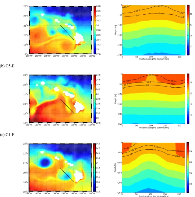
Specific numerical cyclones are chosen, during the last five years of each simulation, because they are spatially and tem-porally representative of cyclone Opal studied during the cruise E-FLUX III (10–28 March 2005). These eddies are compared with each other and with observational data. The different eddy characteristics’ statistics and the ones of cy-clone Opal are summarized in Table 2. Cycy-clones are ex-pected to exhibit an uplift of isopycnal and of isothermal sur-faces. Depending on the runs, these characteristics are more or less apparent (Figs. 9, 10). The sections reveal an intense doming of isothermal and isopycnal surfaces with outcrop-ping at the surface for Run-C and Run-F (Figs. 9c, 10c). This uplift is also present for Run-A, Run-D and Run-E (Figs. 9a, 10a, b) but is not as pronounced as in the previous results. The Run-B results are characterized by smooth isothermal and isopycnal surfaces (Fig. 9b). The deepest depths, where the eddies still influence the isopycnals, vary between 90 m (Run-B) and 250 m (Run-A, Run-C, Run-F). We have cal-culated an estimate of the diameter of the different cyclonic eddies following the method used by Dickey et al. (2008). These diameters vary between 160 km (Run-A) and 210 km (Run-C, Run-D). The diameters for Run-E and Run-F fea-tures are of the same order than the one of cyclone Opal. The
values of the maximum tangential velocities (Table 2) can give us information on the intensity of each cyclones. The Run-A and Run-B results are characterized by the lowest ve-locity (0.23 − 0.24 m s−1), while those of Run-C, Run-D and
Run-F by the highest velocity (0.53 − 0.55 m s−1). An
inter-mediate value is found for the Run-E results (0.30 m s−1).
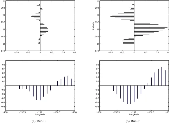
The numerical cyclones of Run-A and Run-B are not en-ergetic enough and those of Run-C and Run-D are too large compared to the characteristics of cyclone Opal. Hence the results of Run-E and Run-F are the closest ones to the Opal characteristics. Hereafter we concentrate on these two runs during the tenth year of simulation. We have calculated the east-west (north-south) components of the horizontal veloc-ity vector along a north-south (east-west) transect for Run-E and Run-F. We report zonal and meridional components of the 40-m depth horizontal velocity along meridional and zonal transects, respectively, for eddies C5-E and C1-F in Fig. 11. We have chosen this depth for a comparison with in situ measurements performed by Nencioli et al. (2008) inside the cyclone Opal.
The position of the center of the eddy can be located at the point of minimal velocity, here near 19.5◦N, 156.6◦W for both eddies (Fig. 12).
In Fig. 13 we show the distribution of the zonal and merid-ional components of the 40-m depth horizontal velocity with respect to the distance from the eddy center for both C5-E (Run-E, 13 April) and C1-F (Run-F, 28 March). Both eddies
286 M. Kersalé et al.: Sensitivity study of the generation of Hawaii mesoscale eddies (a) C3-A 161oW 160oW 159oW 158oW 157oW 156oW 155oW 154oW 18oN 19oN 20oN 21oN 22oN 23oN 22.8 23 23.2 23.4 23.6 23.8 24 24.2 24.4 24.6 24.8 0 50 100 150 200 −250 −200 −150 −100 −50 0
Position along the section [km]
Depth [m] 23.6 23.6 23.6 23.8 23.8 23.8 24 24 24 10 15 20 25 (b) C3-B 161oW 160oW 159oW 158oW 157oW 156oW 155oW 154oW 18oN 19oN 20oN 21oN 22oN 23oN 22.8 23 23.2 23.4 23.6 23.8 24 24.2 24.4 24.6 24.8 0 50 100 150 200 −250 −200 −150 −100 −50 0
Position along the section [km]
Depth [m] 23.6 23.8 23.8 23.8 24 24 24 10 15 20 25 (c) C2-C 161oW 160oW 159oW 158oW 157oW 156oW 155oW 154oW 18oN 19oN 20oN 21oN 22oN 23oN 22.8 23 23.2 23.4 23.6 23.8 24 24.2 24.4 24.6 24.8 0 50 100 150 200 −250 −200 −150 −100 −50 0
Position along the section [km]
Depth [m] 23.6 23.8 23.8 24 24 24 10 15 20 25
Fig. 9. Left : surface temperature maps on March 28 with position of the transects (black straight line) crossing the center of a cyclonic eddy Run-A (top), Run-B (middle) and Run-C (bottom). Right : Corresponding vertical sections of temperature. The black lines in the vertical sections represent σt23.6, σt23.8and σt24isopycnals.
Fig. 9. Left: surface temperature maps on 28 March with position of the transects (black straight line) crossing the center of a cyclonic eddy
Run-A (top), Run-B (middle) and Run-C (bottom). Right: corresponding vertical sections of temperature. The black lines in the vertical sections represent σt23.6, σt23.8and σt24isopycnals.
are characterized by values that increase linearly with dis-tance from the center until peaking and then slowly decaying. For C5-E, the peak value is about 0.35 m s−1, while it nearly reaches 0.60 m s−1for C1-F. The linear part corresponds to the solid-body rotation core of the eddy. Otherwise, both eddies appear quite asymmetric and stretched. Hence it is difficult to define with precision an eddy radius. Nonethe-less, it appears clearly that the part in solid body rotation has a diameter smaller than the one estimated above, following Dickey et al. (2008).
4 Discussion
A series of numerical simulations on the Hawaiian region has been done in order to examine the relative importance of wind and topographic forcings on the general circulation and the generation of the eddies. Depending on the runs, the general pattern of the regional oceanic circulation by Lumpkin (1998) is more or less respected. The ocean cir-culations generated by the model forced by the topographic forcing with the inflow currents and no wind (A, Run-B) do not match with this regional circulation. Moreover, these circulations are not realistic because the intensity of the
M. Kersalé et al.: Sensitivity study of the generation of Hawaii mesoscale eddies 287 (a) C3-D 161oW 160oW 159oW 158oW 157oW 156oW 155oW 154oW 18oN 19oN 20oN 21oN 22oN 23oN 22.8 23 23.2 23.4 23.6 23.8 24 24.2 24.4 24.6 24.8 0 50 100 150 200 −250 −200 −150 −100 −50 0
Position along the section [km]
Depth [m] 23.6 23.8 23.8 23.8 24 24 24 10 15 20 25 (b) C5-E 161oW 160oW 159oW 158oW 157oW 156oW 155oW 154oW 18oN 19oN 20oN 21oN 22oN 23oN 22.8 23 23.2 23.4 23.6 23.8 24 24.2 24.4 24.6 24.8 0 50 100 150 200 −250 −200 −150 −100 −50 0
Position along the section [km]
Depth [m] 23.6 23.6 23.6 23.8 23.8 23.8 24 24 24 10 15 20 25 (c) C1-F 161oW 160oW 159oW 158oW 157oW 156oW 155oW 154oW 18oN 19oN 20oN 21oN 22oN 23oN 22.8 23 23.2 23.4 23.6 23.8 24 24.2 24.4 24.6 24.8 0 50 100 150 200 −250 −200 −150 −100 −50 0
Position along the section [km]
Depth [m] 23.6 23.8 23.8 23.8 24 24 24 10 15 20 25
Fig. 10. Left : surface temperature maps with position of the transects (black straight line) crossing the center of a cyclonic eddy on April 13 for Run-E (middle) and on March 28 for both Run-D (top) and Run-F (bottom). Right : Corresponding vertical sections of temperature. The black lines in the vertical sections represent σt23.6, σt23.8and σt24isopycnals.
Fig. 10. Left: surface temperature maps with position of the transects (black straight line) crossing the center of a cyclonic eddy on April 13
for Run-E (middle) and on 28 March for both Run-D (top) and Run-F (bottom). Right: corresponding vertical sections of temperature. The black lines in the vertical sections represent σt23.6, σt23.8and σt24isopycnals.
eddies is too low (0.23–0.24 m s−1). Both simulations show the importance of inflow current and topographic forcing on oceanic eddy shedding. When the model is forced only by QuickSCAT wind data (Run-C), two stationary eddies and a periodical one develop in the island wake, responding to the vorticity injected by the wind stress curl. The fact that the cyclone is stationary could be due to topographic β-effect (Cushman-Roisin and Beckers, 2011). Hence in our case, the cyclone will tend to move toward the north-east against the islands of Maui and the Big Island. As for the anticyclonic eddy, its position inside the domain so close to the boundary
prevents us to be confident about its behavior. Nevertheless comparing Run-C with Run-D and Run-F (Table 1) the ab-sence of inflow as boundary condition, and hence the abab-sence of NEC, seems to be the reason preventing the westward drift of the anticyclonic eddy. The ocean circulation generated by the model forced by QuickSCAT, but without drag coefficient (Run-D), complies with the circulation of Lumpkin (1998) but with larger eddies than the realistic ones. It implies that the effect of a drag coefficient leads to the compactness of the structures. Nevertheless, in July and August, several intense eddies have been generated in Run-D. During this period,
288 M. Kersalé et al.: Sensitivity study of the generation of Hawaii mesoscale eddies 161oW 160oW 159oW 158oW 157oW 156oW 155oW 154oW 18oN 19oN 20oN 21oN 22oN 23oN −4 −3 −2 −1 0 1 2 3 4 x 10⁻⁵ (a) Run-E 161oW 160oW 159oW 158oW 157oW 156oW 155oW 154oW 18oN 19oN 20oN 21oN 22oN 23oN −4 −3 −2 −1 0 1 2 3 4 x 10⁻⁵ (b) Run-F
Fig. 11. Relative vorticity field at 40-m depth with position of the transects (black straight line) of the eddy C5-E (Run-E, April 13, left) and of the eddy C1-F (Run-F, March 28, right).
Fig. 11. Relative vorticity field at 40-m depth with position of the transects (black straight line) of the eddy C5-E (Run-E, 13 April, left) and
of the eddy C1-F (Run-F, 28 March, right).
20 Kersalé et al.: Sensitivity study of the generation of Hawaii mesoscale eddies
−0.4 −0.2 0 0.2 0.4 0.6 17.5 18 18.5 19 19.5 20 20.5 21 Latitude −0.4 −0.2 0 0.2 0.4 0.6 17.5 18 18.5 19 19.5 20 20.5 21 Latitude −158 −157.5 −157 −156.5 −156 −0.5 −0.4 −0.3 −0.2 −0.1 0 0.1 0.2 0.3 0.4 0.5 Longitude (a) Run-E −158 −157.5 −157 −156.5 −156 −0.5 −0.4 −0.3 −0.2 −0.1 0 0.1 0.2 0.3 0.4 0.5 Longitude (b) Run-F
Fig. 12. East-west horizontal velocity [m s−1] component at 40-m depth vector across a north-south transect (top) and north-south horizontal velocity component across a east-west transect (bottom) of the eddy C5-E (Run-E, April 13, left) and of the eddy C1-F (Run-F, March 28, right).
Fig. 12. East-west horizontal velocity [m s−1] component at 40-m depth vector across a north-south transect (top) and north-south horizontal velocity component across a east-west transect (bottom) of the eddy C5-E (Run-E, 13 April, left) and of the eddy C1-F (Run-F, 28 March, right).
wind forcing is the strongest of the year and acts as a trigger mechanism even when the drag coefficient is set to zero. The ocean circulations generated by the model forced by COADS (Run-E) and QuickSCAT data (Run-F) agree with the known circulation. The annually averaged large-scale circulations are roughly composed of cyclonic eddies to the north and an-ticyclonic eddies to the south, separated by the HLCC. This
is due to the fact that wind, inflow current and topographic forcings act together leading to the same effect. Indeed these three forcings have a cumulative effect while each forcing, taken independently, is not able to create the known circu-lation. This fact is in agreement with the experiments of Jiménez et al. (2008) applied to the case of eddies shed by the island of Gran Canaria. Nevertheless the study of mesoscale
M. Kersalé et al.: Sensitivity study of the generation of Hawaii mesoscale eddies 289 18 18.2 18.4 18.6 18.8 19 19.2 19.4 19.60 0.1 0.2 0.3 0.4 0.5
Latitude South of the center
19.6 19.8 20 20.2 20.4 20.6 20.8 21 21.2 0 0.1 0.2 0.3 0.4 0.5 Latitude North of the center
18 18.2 18.4 18.6 18.8 19 19.2 19.4 19.60 0.1 0.2 0.3 0.4 0.5
Latitude South of the center
19.6 19.8 20 20.2 20.4 20.6 20.8 21 21.2 0 0.1 0.2 0.3 0.4 0.5 Latitude North of the center
−157.8 −157.6 −157.4 −157.2 −157 −156.8 −156.60 0.1 0.2 0.3 0.4 0.5
Longitude West of the center
−156.4 −156.2 −156 −155.8 −155.6 −155.4 0 0.1 0.2 0.3 0.4 0.5 Longitude East of the center
(a) Run-E −157.8 −157.6 −157.4 −157.2 −157 −156.8 −156.60 0.1 0.2 0.3 0.4 0.5
Longitude West of the center
−156.4 −156.2 −156 −155.8 −155.6 −155.4 0 0.1 0.2 0.3 0.4 0.5 Longitude East of the center
(b) Run-F
Fig. 13. Distribution of zonal (top) and meridional (bottom) components of the 40-m depth horizontal velocity [m s−1] with respect to the center of the eddy C5-E (Run-E, April 13, left) and of the eddy C1-F (Run-F, March 28, right).
Fig. 13. Distribution of zonal (top) and meridional (bottom) components of the 40-m depth horizontal velocity [m s−1] with respect to the center of the eddy C5-E (Run-E, 13 April, left) and of the eddy C1-F (Run-F, 28 March, right).
structures in Run-F, based on snapshots (3-days averaged), reveals the splitting of the lee of the Hawaiian Island into two zonal areas, anticyclonic (cyclonic) eddies dominating south (north) of 19◦N. This is in agreement with the regional circu-lation observed by Lumpkin (1998), but shifted half a degree south. The resolution of the dataset considered by Lump-kin (1998) may not be sufficient to reproduce the details of the smaller eddies observed south of the Alenuihaha Chan-nel. Moreover, in our case, we observe that the generation of cyclonic eddies at the northwestern tip of the Big Island is rare (Run-F). Hence we agree with Yoshida et al. (2010) affirming that both positive and negative SSH eddy signals are generated southwest of the Big Island.
Significant differences appear between Run-E and Run-F and have to be noted. A higher temporal variability of the ki-netic energy appears clearly in Run-F with respect to Run-E. Since both simulations seem to satisfy the ergodic hypothe-sis, we think that this temporal variability is induced by the higher spatial variability of the QuickSCAT wind forcing.
In-deed, the similarity between EKE and TKE, in both Run-E and Run-F, indicates that most of the wind forcing momen-tum feeds mesoscale phenomena and that the high values of TKE in the lee of the islands are locally generated. In agree-ment with Calil et al. (2008), our model results show that having good spatial resolution for the surface momentum forcing is vital to produce realistic levels of kinetic energy and vorticity in the ocean circulation. With respect the 14◦ QuickSCAT climatology, the 12◦COADS one does not pro-duce the wind acceleration through the Alenuihaha Channel and other passages between islands.
In the same area, period and conditions of the E-FLUX III field campaigns (i.e. in March and April, downwind of the Alenuihaha Channel and during strong, persistent north-easterly trade winds), our model generates cyclonic eddies in all the simulations. Concerning in situ data, the eddy
Opal, an intense feature, was likely in a well-developed
seg-ment of its lifetime when it was measured with a diameter of 180–200 km and a maximum velocity of around 0.6 m s−1
outcropping to the surface (Dickey et al., 2008). We then compare the modeled cyclonic cold-core eddies with respect to the observations of the eddy Opal. For A and Run-B, both cyclones show an outcropping of the isopycne σt23.6
to the surface. But the uplift of the isotherms is more pro-nounced in Run-A than in Run-B. This fact can be explained by a homogenization when the current is more intense. For Run-C, the wind stress curl causes the development of cy-clonic eddies by forcing strong Ekman pumping, which leads to water upwelling. The isothermal and isopycnal uplift is the strongest of the six simulations. Because of the Ekman pumping, it is possible that the wind forcing has a greater impact upon the strength of the upwelling in the immediate lee region, as suggested by Yoshida et al. (2010). We have concentrated on the two cyclonic eddies of E and Run-F because they correspond to the most realistic simulations. The model reproduces well the intense doming of isothermal and isopycnal associated with the cyclonic structures. Calil et al. (2008) said that the model forced by COADS climatol-ogy did not produce significant isolated mesoscale cyclonic eddies. In our model, Run-E cyclones are produced but ap-pear smaller in diameter and less energetic than Run-F ones and Opal. Moreover the maximum velocity in Run-F cy-clones are higher than the Run-E one and closer in amplitude to the maximum velocities measured in Opal (Nencioli et al., 2008). The behavior of the simulated cyclonic eddy is sim-ilar to that observed, but the southward drift of Opal is well reproduced only by C1-F.
5 Conclusions
The Hawaiian archipelago has a strong influence on both the atmospheric and the oceanic circulations. In this study, we performed several experiments to study the relative im-portance of topographic and wind forcings on oceanic eddy shedding by the Hawaiian archipelago. We have compared the oceanic circulation around Hawaii and have obtained sig-nificant differences between the simulations using different forcings. This study demonstrates the need for the presence of the three forcings (wind, inflow current and topography) to reproduce the oceanic circulation. These forcings have a cumulative effect on the generation of mesoscale eddies and lead to a complex oceanic circulation pattern. While each forcing, taken independently, is not able to create the known circulation. The wind stress curl, via the Ekman pumping mechanism, has also been identified as an important mecha-nism upon the strength of the upwelling in the immediate lee region. In order to well reproduce the oceanic circulation in the area, it is necessary to have, not only a high spatial reso-lution for the circulation model, but also a wind stress forcing data that reproduces the complexity of the atmospheric flow between the islands. In agreement with previous numerical
simulation forced by QuikSCAT wind data (Run-F) repro-duces well the energetic mesoscale structures observed dur-ing the E-FLUX field experiments (Dickey et al., 2008), in-cluding their hydrological characteristics and behavior. This setup will allow future studies that are needed to better un-derstand the role of temporal variability on the behavior of mesoscale eddies and the role of these structures in the dis-tribution of biogeochemical properties.
Acknowledgements. M. Kersalé thanks the “Service Informatique
du COM (SIC)” for their assistance in the students’ computer facility. The authors want to thank I. Dekeyser and F. Nencioli for precious comments and useful discussions. The authors also thank the numerous anonymous reviewers for their constructive remarks and suggestions. This work is in the framework of the LATEX project (http://www.com.univ-mrs.fr/LOPB/LATEX), founded by CNRS LEFE/IDAO-CYBER and Région PACA.
Edited by: K. J. Heywood
References
Aristegui, J., Sangra, P., Henandez-Leon, S., Canton, M., and Hernandez-Guerra, A.: Island-induced eddies in the Canary Is-lands, Deep-Sea Res. Pt. I, 41, 1509–1525, 1994.
Aristegui, J., Tett, P., Hernandez-Guerra, A., Basterretxea, G., Mon-tero, M. F., Wild, K., Sangra, P., Hernandez-Leon, S., Can-ton, M., Garcia-Braun, J. A., Pacheco, M., and BarCan-ton, E. D.: The influence of island-generated eddies on chlorophyll distribu-tion: a study of mesoscale variation around Gran Canaria, Deep-Sea Res. Pt. I, 44, 71–96, 1997.
Barton, E., Basterretxea, G., Flament, P., Mitchelson-Jacob, E., Jones, B., Aristegui, J., and Herrera, F.: Lee region of Gran Ca-naria, J. Geophys. Res., 105, 17173–17193, 2000.
Beckmann, A. and Haidvogel, D.: Numerical simulation of flow around a tall isolated seamount. Part 1: Problem formulation and model accuracy, J. Phys. Oceanogr., 23(8), 1736–1753, 1993. Bidigare, R. R., Benitez-Nelson, C., Leonard, C. L., Quay, P. D.,
Parsons, M. L., Foley, D. G., and Seki, M. P.: Influence of a cyclonic eddy on microheterotroph biomass and carbon export in the lee of Hawaii, Geophys. Res. Lett., 30, 1318, doi:10.1029/2002GL016393, 2003.
Blanke, B., Speich, S., Bentamy, A., Roy, C., and Sow, B.: Mod-eling the structure and variability of the southern Benguela up-welling using QuikSCAT wind forcing, J. Geophys. Res., 110, C07018, doi:10.1029/2004JC002529, 2005.
Calil, P. H. R., Richards, K. J., Yanli, J., and Bidigare, R. R.: Eddy activity in the lee of the Hawaiian Islands, Deep-Sea Res. Pt. II, 55, 1179–1194, 2008.
Callahan, P. S. and Lungu, T.: QuikSCAT Science Data Product User’s Manual (v3.0), Tech. rep., Jet Propul. Lab., Pasadena, CA, 91 pp., 2006.
Chavanne, C., Flament, P., Lumpkin, R., Dousset, B., and Bentamy, A.: Scatterometer observations of wind variations induced by oceanic islands: implications for wind-driven ocean circulation, Can. J. Remote Sens., 28, 466–474, 2002.
Chelton, D. B., deSzoeke, R. A., Schlax, M. G., El Naggar, K., and Siwertz, N.: Geographical variability of the first-baroclinic Rossby radius of deformation, J. Phys. Oceanogr., 28, 433–460, 1998.
Cherniawsky, J. Y. and Crawford, W. R.: Comparison between weather buoy and Comprehensive Ocean-Atmosphere Data Set wind data for the west coast of Canada, J. Geophys. Res., 101, 18377–18390, 1996.
Cushman-Roisin, B.: Introduction to Geophysical Fluid Dynamics, Prentice-Hall, Upper Saddle River, N. J., 320 pp., 1994. Cushman-Roisin, B. and Beckers, J. M.: Introduction to
Geophysi-cal Fluid Dynamics: PhysiGeophysi-cal and NumeriGeophysi-cal Aspects, Academic Press, September 2011.
Da Silva, A. M., Young, C. C., and Levitus, S.: Atlas of surface marine data 1994, vol. 1, algorithms and procedures, Tech. rep., U.S. Department of Commerce, NOAA, 1994.
Dickey, T. D., Nencioli, F., Kuwahara, V. S., Leonard, C., Black, W., Rii, Y. M., Bidigare, R. R., and Zhang, Q.: Physical and bio-optical observations of oceanic cyclones west of the island of Hawaií, Deep-Sea Res. Pt. II, 55, 1195–1217, 2008.
Dong, C. and McWilliams, J. C.: A numerical study of island wakes in the Southern California Bight, Cont. Shelf Res., 27, 1233– 1248, doi:10.1016/j.csr.2007.01.016, 2007.
Dong, C., Mavor, T., Nencioli, F., Jiang, S., Uchiyama, Y., McWilliams, J. C., Dickey, T. D., Ondrusek, M., Zhang, H., and Clark, D. K.: An oceanic eddy on the lee side of Lanai Island, Hawai’i, J. Geophys. Res., 114, C10008, doi:10.1029/2009JC005346, 2009.
Firing, Y. L. and Merrifield, M. A.: Extreme sea level events at Hawaii: Influence of mesoscale eddies, Geophys. Res. Lett., 31, L24306, doi:10.1029/2004GL021539, 2004.
Jiménez, B., Sangrà, P., and Mason, E.: A numerical study of the relative importance of wind and topographic forcing on oceanic eddy shedding by tall, deep water islands, Ocean Model., 22, 146–157, doi:10.1016/j.ocemod.2008.02.004, 2008.
Lumpkin, C. F.: Eddies and currents in the Hawaii islands, Ph.D. thesis, University of Hawaii, 1998.
Marchesiello, P., McWilliams, J. C., and Shchepetkin, A.: Open boundary condition for long-term integration of regional oceanic models, Ocean Model., 3, 1–21, doi:10.1016/S1463-5003(00)00013-5, 2001.
Monaldo, F. M., Thompson, D. R., Pichel, W. G., and Clemente-Colon, P.: A systematic comparison of QuikSCAT and SAR ocean surface wind speeds, IEEE T. Geosci. Remote, 42, 283– 291, 2004.
Morrow, R., Birol, F., Griffin, D., and Sudre, J.: Divergent pathways of cyclonic and anti-cyclonic ocean eddies, Geophys. Res. Lett., 31, L24311, doi:10.1029/2004GL020974, 2004.
Nencioli, F., Kuwahara, V. S., Dickey, T. D., Rii, Y. M., and Bidi-gare, R. R.: Physical dynamics and biological implications of a mesoscale eddy in the lee of Hawai’i: Cyclone Opal observations during E-FLUX III, Deep-Sea Res. Pt. II, 55, 1252–1274, 2008.
Patzert, W. C.: Eddies in Hawaiian Islands, Tech. rep., Hawaii In-stitute of Geophysics, University of Hawaii, 1969.
Penven, P., McWilliams, J. C., Marchesiello, P., and Chao, Y.: Coastal Upwelling response to atmospheric wind forcing along the Pacific coast of the United States, Ocean Sciences Meeting, Honolulu, Hawaii (USA), 2002.
Penven, P., Cambon, G., Tan, T. A., Marchesiello, P., and Debreu, L.: ROMSTOOLS user guide, Tech. rep., Inst. de Rech. pour le Dév., Marseille, France, http://roms.mpl.ird.fr, 2010.
Qiu, B., Koh, D. A., Lumpkin, C., and Flament, P.: Existence and formation mechanism of the North Hawaiian Ridge Current, J. Phys. Oceanogr., 27, 431–444, 1997.
Renfrew, I. A., Petersen, G. N., Sproson, D. A. J., Moore, G. W. K., Adiwidjaja, H., Zhang, S., and North, R.: A compar-ison of aircraft-based surface-layer observations over Denmark Strait and the Irminger Sea with meteorological analyses and QuikSCAT winds, Q. J. Roy. Meteor. Soc., 135, 2046–2066, 2009.
Seki, M. P., Polovina, J. J., Brainard, R. E., Bidigare, R. R., Leonard, C. L., and Foley, D. G.: Biological enhancement at cy-clonic eddies tracked with GOES thermal imagery in Hawaiian waters, Geophys. Res. Lett., 28, 1583–1586, 2001.
Seki, M. P., Lumpkin, R., and Flament, P.: Hawaii cyclonic ed-dies and blue marlin catches: the case study of the 1995 Hawai-ian International Billfish Tournament, J. Oceanogr., 58, 739–745, 2002.
Shchepetkin, A. F. and McWilliams, J. C.: A method for com-puting horizontal pressure-gradient force in an oceanic model with nonaligned vertical coordinate, J. Geophys. Res., 108, 3090, doi:10.1029/2001JC001047, 2003.
Shchepetkin, A. F. and McWilliams, J. C.: The regional oceanic modeling system (ROMS): a split-explicit, free-surface, topography-following-coordinate oceanic model, Ocean Model., 9, 347–304, doi:10.1016/j.ocemod.2004.08.002, 2005.
Smith, R. B. and Grubisic, V.: Aerial observations of Hawaii’s wake, J. Atmos. Sci., 50, 3728–3750, 1993.
Smith, W. H. F. and Sandwell, D. T.: Global sea floor topography from satellite altimetry and ship depth soundings, Science, 227, 1956–1962, doi:10.1126/science.277.5334.1956, 1997. Wu, R. and Xie, S.: On Equatorial Pacific surface wind changes
around 1977: NCEP-NCAR reanalysis versus COADS observa-tions, J. Climate, 16, 167–173, 2003.
Xie, S., Liu, W., Liu, Q., and Nonaka, M.: Far-Reaching Effects of the Hawaiian Islands on the Pacific Ocean-Atmosphere System, Science, 292, 2057–2060, 2001.
Yoshida, S., Qiu, B., and Hacker, P.: Wind-generated eddy charac-teristics in the lee of the island of Hawaii, J. Geophys. Res., 115, C03019, doi:10.1029/2009JC005417, 2010.
Zdravkovich, M. M.: Flow around Circular Cylinders: A Compre-hensive Guide through Flow Phenomena, Experiments, Applica-tions, Mathematical Models, and Computer SimulaApplica-tions, Oxford University Press, New York, 694 pp., 1997.
![Fig. 1. Model domain and bathymetry [m]. Names of the islands and coastline at higher resolution are reported for geographical in-formation.](https://thumb-eu.123doks.com/thumbv2/123doknet/14781737.596868/4.892.74.428.96.335/model-bathymetry-islands-coastline-resolution-reported-geographical-formation.webp)
![Fig. 2. Temporal evolutions (model time, years) of volume-averaged kinetic energy [cm 2 s −2 ] for the six numerical experiments](https://thumb-eu.123doks.com/thumbv2/123doknet/14781737.596868/5.892.146.747.93.472/temporal-evolutions-volume-averaged-kinetic-energy-numerical-experiments.webp)