Star Formation in Galaxies at z ∼ 4–5 from the SMUVS Survey: A Clear Starburst/Main-sequence Bimodality for Hα Emitters on the SFR–M* Plane

HAL Id: hal-01645708

https://hal.archives-ouvertes.fr/hal-01645708

Submitted on 3 May 2018

HAL is a multi-disciplinary open access

archive for the deposit and dissemination of

sci-entific research documents, whether they are

pub-lished or not. The documents may come from

teaching and research institutions in France or

abroad, or from public or private research centers.

L’archive ouverte pluridisciplinaire HAL, est

destinée au dépôt et à la diffusion de documents

scientifiques de niveau recherche, publiés ou non,

émanant des établissements d’enseignement et de

recherche français ou étrangers, des laboratoires

publics ou privés.

Star Formation in Galaxies at z

∼ 4–5 from the SMUVS

Survey: A Clear Starburst/Main-sequence Bimodality

for Hα Emitters on the SFR–M* Plane

K.I. Caputi, S. Deshmukh, M.L.N. Ashby, W.I. Cowley, L. Bisigello, G.G.

Fazio, J.P.U. Fynbo, O. Le Fèvre, B. Milvang-Jensen, O. Ilbert

To cite this version:

K.I. Caputi, S. Deshmukh, M.L.N. Ashby, W.I. Cowley, L. Bisigello, et al.. Star Formation in Galaxies

at z

∼ 4–5 from the SMUVS Survey: A Clear Starburst/Main-sequence Bimodality for Hα Emitters on

the SFR–M* Plane. Astrophys.J., 2017, 849 (1), pp.45. �10.3847/1538-4357/aa901e�. �hal-01645708�

STAR FORMATION IN GALAXIES AT z ∼ 4 − 5 FROM THE SMUVS SURVEY: A CLEAR

STARBURST/MAIN-SEQUENCE BIMODALITY FOR Hα EMITTERS ON THE SFR − M∗ PLANE

K. I. Caputi,1 S. Deshmukh,1 M. L. N. Ashby,2 W. I. Cowley,1 L. Bisigello,1 G. G. Fazio,2 J. P. U. Fynbo,3 O. Le F`evre,4 B. Milvang-Jensen,3 and O. Ilbert4

1_{Kapteyn Astronomical Institute, University of Groningen, P.O. Box 800, 9700AV Groningen, The Netherlands} 2_{Harvard-Smithsonian Center for Astrophysics, 60 Garden St., Cambridge, MA 02138, USA}

3_{Dark Cosmology Centre, Niels Bohr Institute, University of Copenhagen, Juliane Maries Vej 30, 2100 Copenhagen, Denmark} 4_{Aix Marseille Universit´e, CNRS, LAM (Laboratoire d’Astrophysique de Marseille), UMR 7326, 13388, Marseille, France}

(Received ...; Revised ...; Accepted ...)

Submitted to ApJ ABSTRACT

We study a large galaxy sample from the Spitzer Matching Survey of the UltraVISTA ultra-deep Stripes (SMUVS) to search for sources with enhanced 3.6 µm fluxes indicative of strong Hα emission at z = 3.9 − 4.9. We find that the percentage of “Hα excess” sources reaches 37-40% for galaxies with stellar masses log10(M∗/M) ≈ 9 − 10, and

decreases to < 20% at log10(M∗/M) ∼ 10.7. At higher stellar masses, however, the trend reverses, although this is

likely due to AGN contamination. We derive star formation rates (SFR) and specific SFR (sSFR) from the inferred Hα equivalent widths (EW) of our “Hα excess” galaxies. We show, for the first time, that the “Hα excess” galaxies clearly have a bimodal distribution on the SFR-M∗ plane: they lie on the main sequence of star formation (with log10(sSFR/yr−1) < −8.05) or in a starburst cloud (with log10(sSFR/yr−1) > −7.60). The latter contains ∼ 15%

of all the objects in our sample and accounts for > 50% of the cosmic SFR density at z = 3.9 − 4.9, for which we derive a robust lower limit of 0.066 Myr−1Mpc−3. Finally, we identify an unusual > 50σ overdensity of z = 3.9 − 4.9

galaxies within a 0.20 × 0.20 arcmin2 region. We conclude that the SMUVS unique combination of area and depth at mid-IR wavelengths provides an unprecedented level of statistics and dynamic range which are fundamental to reveal new aspects of galaxy evolution in the young Universe.

Keywords: galaxies: high-redshift, galaxies: star formation, galaxies: starburst, galaxies: evolution, infrared: galaxies

Corresponding author: K. I. Caputi [email protected]

Caputi et al.

1. INTRODUCTION

Studying star formation in galaxies at high redshifts is crucial to understanding the early stages of galaxy evolu-tion. Over the last ten years, a picture has emerged indi-cating that the global cosmic star formation rate (SFR) density increased after the Big Bang until reaching a peak about ten billion years ago, and then declined un-til today (e.g.Hopkins & Beacom 2006;Behroozi et al. 2013; Madau & Dickinson 2014). That peak is likely the product of two effects: mainly the net increase in the number density of galaxies that make the bulk of star formation in the first few billion years and possibly, but this is less clear, the fact that the SFR of individual galaxies may increase over that time. Indeed, our cur-rent knowledge of how star formation and stellar mass buildup proceeded over the first few billion years is still very sparse.

In most observed star-forming galaxies up to at least z ∼ 3, the instantaneous SFR appears to correlate (within some scatter) with the stellar mass. This cor-relation on the SFR-M∗ plane is the so-called ‘galaxy star-formation main sequence’ (e.g.,Noeske et al. 2007;

Rodighiero et al. 2010; Elbaz et al. 2011). For these galaxies the specific star formation rates (sSFR≡ SFR/M∗) are roughly constant, which implies the ex-istence of a scaling relation between gas consumption and galaxy growth (see e.g., Popping et al. 2015; La-gos et al. 2016). In addition, there exists a minority of star-forming galaxies which are characterised by signifi-cantly higher sSFRs and are usually called ‘starbursts’. The starburst phase is presumably a temporary state in which the galaxy is taken out of the main sequence, due to some kind of perturbation that temporarily enhances the star formation. Starburst galaxies are very rare in the local Universe and have been found to constitute a small fraction of the dusty star-forming galaxies ob-served at redshifts z ∼ 0.3 to z ∼ 2 (Rodighiero et al. 2011; Sargent et al. 2012). This inferred weak evolu-tion in the starburst fracevolu-tion with redshift is based on the analysis of the most luminous dusty galaxies, as only these galaxies could be detected by the last generation of infrared (IR) telescopes, particularly the Herschel Space Telescope. Therefore, these results mainly concern mas-sive galaxies and it is not obvious whether they can be extrapolated to all star-forming galaxies.

A main limiting factor to understanding galaxy evo-lution in the high-z Universe has been the lack of deep galaxy surveys over significantly large areas of the sky. Such surveys could provide sufficient statistics and dy-namic range to investigate how star formation, as well as different physical properties, vary among different stellar-mass galaxies. For star formation, in particular,

another limitation is that the only tracer currently avail-able for large galaxy samples is the rest-ultraviolet (UV) flux shifted into observed optical wavelengths at high-z. UV fluxes are extremely sensitive to dust extinction and, thus, the derived SFRs can be very uncertain. Far-IR and (sub)-millimetre photometry are the ideal comple-ment to UV photometry for the purpose of obtaining total SFR estimates, but single-dish far-IR telescopes are insufficiently sensitive to systematically study rep-resentative galaxy samples in the high-z Universe. As an alternative, Balmer lines, especially Hα λ6563, which is much less affected by dust than the UV spectral con-tinuum, is a very suitable SFR tracer widely used for galaxies up to z ∼ 2 − 3. However, Hα is shifted into the mid-IR regime (λ >_{∼ 3 µm) at z > 3, making its} de-tection prohibitive for current spectrographs.

When emission lines have sufficiently large equiva-lent widths (EW), however, their presence can be in-ferred even from broad-band photometry. At redshifts 3.9 <_{∼ z}<

∼ 4.9, the Hα line is encompassed by the 3.6 µm filter passband at the Infrared Array Camera (IRAC;

Fazio et al. 2004) on board the Spitzer Space Telescope (Werner et al. 2004). This fact has been exploited by different authors to investigate the presence of intense Hα emitters at these redshifts. Shim et al. (2011) ana-lyzed a sample of 74 galaxies at similar redshifts and con-cluded that ∼ 70% of these galaxies have an excess flux at 3.6 µm with respect to the stellar continuum. More recently,Stark et al. (2013) andSmit et al. (2016) con-ducted similar analyses, based on galaxy samples with spectroscopic and photometric redshifts, and confirmed the presence of intense Hα emitters at z ∼ 4 − 5. The percentage of galaxies displaying an “Hα excess” and the derived rest EWs varied according to the different selection effects, but in general they found median val-ues of Hα EW≈ 300 − 400 ˚A. These EWs are on average much larger than those observed in the local Universe and are broadly consistent with an increase with red-shift, as determined by Fumagalli et al. (2012), Faisst et al. (2016) and M´armol-Queralt´o et al. (2016). All these studies have been very valuable to raise awareness on the increasing importance of nebular emission up to at least z ∼ 5. However, none of them has analyzed a sufficiently representative galaxy sample at z ∼ 4 − 5, which would allow for a more complete investigation of the implications of these results within the context of galaxy evolution.

The Spitzer Matching Survey of the Ultra-VISTA ultra-deep Stripes (SMUVS; M. Ashby et al., 2017, in preparation) is a Spitzer Exploration Science Program which has collected ultra-deep IRAC 3.6 and 4.5 µm images over a significant part of the COSMOS field

(Scoville et al. 2007), making it the largest quasi-contiguous Spitzer field to analyze the high-z Universe. The SMUVS unprecedented level of statistics allows for a detailed study of galaxy properties and evolution over more than three decades in stellar mass at high z. In this paper we analyze the large SMUVS galaxy sample containing almost 6000 sources at 3.9 ≤ z ≤ 4.9 to investigate the presence of prominent Hα emitters as a function of stellar mass, along with the implications for the SFR versus M∗relation at those high redshifts.

This paper is organised as follows. In Section §2 we describe the utilised datasets, source catalogue construc-tion, as well as photometric redshifts and stellar mass derivations. In Section §3 we explain our selection cri-teria for “Hα excess” galaxies among all SMUVS galax-ies at 3.9 ≤ z ≤ 4.9. In Section §4 we present our results on the derived nebular line equivalent widths; SFRs and resulting SFR-M∗ and sSFR-M∗ relations; and the inferred cosmic star formation rate density at z ∼ 4 − 5. We also discuss a rare z ∼ 4 − 5 overdensity in the SMUVS field. Finally, in Section

5 we summarize our findings and discuss our conclu-sions. Throughout this paper we adopt a cosmology with H0 = 70 km s−1Mpc−1, ΩM = 0.3 and ΩΛ = 0.7.

All magnitudes and fluxes are total, with magnitudes referring to the AB system (Oke & Gunn 1983). Stel-lar masses correspond to aChabrier (2003) initial mass function (IMF), except where explicitly stated otherwise (see Section §4.3).

2. DATASETS AND PHOTOMETRIC REDSHIFTS

The SMUVS program (PI Caputi; M. Ashby et al., 2017, in preparation) has collected ultra-deep Spitzer 3.6 and 4.5 µm data over the region of the COSMOS field (Scoville et al. 2007) overlapping the three Ul-traVISTA ultra-deep stripes (McCracken et al. 2012) with deepest optical coverage from the Subaru telescope (Taniguchi et al. 2007). The SMUVS mosaics utilised here correspond to the survey almost final depth, which reaches an average integration time of ∼ 25 h/pointing (including previously available IRAC data in COSMOS;

Sanders et al. 2007; Ashby et al. 2013; Steinhardt et al. 2014; Ashby et al. 2015). The considered UltraV-ISTA data correspond to the third data release (DR3), which in the ultra-deep stripes reaches an average depth of Ks= 24.9±0.1 and H = 25.1±0.1 (200diameter; 5σ)1.

A complete description of our SMUVS source multi-wavelength catalogue construction and spectral energy distribution (SED) fitting is provided in S. Deshmukh

1_{see http://www.eso.org/sci/observing/phase3/data releases/} uvista dr3.pdf

et al. (2017, in preparation). Here we only summarize our main steps. Firstly, we extracted sources on Ultra-VISTA HKs average stack mosaics of the three rele-vant ultra-deep stripes, using the software SExtractor (Bertin & Arnouts 1996) with a detection threshold of 1.5σ over 5 contiguous pixels. The position of these sources were considered as priors to perform iterative PSF-fitting photometric measurements on the Spitzer SMUVS 3.6 and 4.5 µm mosaics, using the DAOPHOT package on IRAF with empirical point-spread-functions (PSFs) obtained from stars in the field (in each stripe separately). The PSF-fitting algorithm converged for ∼ 70% of the sources. For the remaining ones, we measured directly IRAC aperture fluxes in 2.4 arcsec-diameter circular apertures at the position of the Ultra-VISTA sources, and corrected them to total fluxes mul-tiplying by a factor of 2.13, which was determined from the curves of growth of stars in the field. Overall, we found that ∼ 95 − 96% of the UltraVISTA ultra-deep sources are detected in at least one IRAC band (and 93 − 94% in both bands). The comparison of the re-sulting IRAC number counts with those obtained in the deeper S-CANDELS survey (Ashby et al. 2015) indi-cates that our resulting SMUVS catalogue is 80%(50%) complete at [3.6] and [4.5]=25.5 (26.0) total magnitudes. For all these sources, we measured 2-arcsec diameter circular photometry on 26 broad, intermediate and nar-row bands from the U through the Ksbands, using

SEx-tractor on dual-image mode with the UltraVISTA HKs stacks as detection images, and applied corresponding point-source aperture corrections in each band. After cleaning for galactic stars based on a (J -[3.6]) versus (B-J ) colour-colour diagram (e.g., Caputi et al. 2011) and masking regions of contaminated light around the brightest sources, our final catalogue contains ∼ 291, 300 UltraVISTA sources with at least one IRAC-band detec-tion over a net area of 0.66 deg2_{. This is our SMUVS}

parent catalogue with 28-band photometry (U through Ks+ IRAC) for SED fitting analysis.

The PSF-fitting technique assumes that all sources are point-like: on the IRAC images, this is indeed a reasonable assumption for virtually all sources with [3.6] > 21 mag (see Fig. 25 in Ashby et al. 2013). Besides, all the multi-wavelength photometry that we considered for SED fitting has been measured on cir-cular apertures (and corrected to total), so the IRAC photometry based on PSF fitting is consistent with this procedure.

We performed the source SED fitting using the χ2

-minimization code LePhare (Arnouts et al. 1999;Ilbert et al. 2006) over our 2-arcsec-based total flux source catalogue. We used Bruzual & Charlot (2003) templates

Caputi et al. corresponding to a single stellar population and different

exponentially declining star formation histories (SFHs), all with solar metallicity (Z), allowing for the addition

of emission lines. In Appendix A, we discuss the impact of considering two possible metallicities (Zand 0.2 Z)

for the SED fitting. To account for internal dust extinc-tion, we used the Calzetti et al. (2000) reddening law. Throughout this paper we will consider that the extinc-tion derived in this way from the SED fitting of each galaxy is the same for the spectral continuum and lines at the same wavelengths, which should be a reasonable assumption for the majority of our galaxies (e.g.,Reddy et al. 2010;Shivaei et al. 2015). In Appendix B, we ex-plore the effects of assuming a different dust-extinction law which is directly dependent on the UV slope of each galaxy.

As in Caputi et al. (2015), in the case of non-detections we adopted 3σ flux upper limits in the broad bands and ignored narrow and intermediate bands. For the minority (< 14%) of sources corresponding to [3.6] or [4.5]> 22 galaxies with a [3.6] or [4.5]< 23 neighbour within a 3 arcsec radius, we performed the SED fitting only on 26 bands (ignoring the IRAC bands).

We obtained zero-point corrections to the photome-try from a first LePhare run and then we performed a second, definitive run taking into account these correc-tions. From LePhare’s output we obtained photomet-ric redshifts and stellar mass estimates for > 99.9% of our sources. The COSMOS field has a large amount of spectroscopic data which are very useful to assess the quality of the obtained photometric redshifts (e.g.,

Lilly et al. 2007): the resulting dispersion of the |zphot

-zspec|/(1 + zspec) distribution in our sample, based on

∼14,000 galaxies with reliable spectroscopic redshifts, is σ = 0.026 with 5.5% outliers (S. Deshmukh et al., 2017, in preparation). This general photometric red-shift quality is similar to that restricted to the redred-shift range analyzed here, i.e., 3.9 ≤ z ≤ 4.9. At these high redshifts we have 55 sources with spectroscopic redshifts and obtain σ = 0.023 with 7.3% outliers.

From the obtained SMUVS photometric redshift cat-alogue, we excluded ∼ 1% of sources because their best-fit zphotwere incompatible with their detection at short

wavelengths – see criteria in Caputi et al. (2015). Our final SMUVS catalogue with photometric redshift deter-minations contains 288,003 galaxies, including 5925 at 3.9 ≤ z ≤ 4.9, which is the relevant redshift range in this work. As part of LePhare’s output, we also have stellar mass estimates for all these sources.

3. SELECTION OF PROMINENT Hα EMITTERS

AT z = 3.9 − 4.9

At redshifts 3.9 ≤ z ≤ 4.8 the entire (Hα λ6563+ +[NII] λλ6548, 6583+ [SII] λλ6716, 6730) emission line complex is encompassed within the IRAC 3.6 µm filter and the (Hα λ6563 + [NII] λλ6548, 6583) complex is present up to z ≈ 4.9. At these same redshifts, no promi-nent emission line is present in the IRAC 4.5 µm filter. At z >_{∼ 4.4, the [OII] λλ3727 enters the K}s band,

al-though its EW is typically significantly smaller than the Hα EW (e.g.,Mouhcine et al. 2005). The (Hβ λ4861 + [OIII] λλ5007) complex lies in the gap between the Ks

and 3.6 µm bands.

Only emission lines or line complexes with sufficiently large EW can produce a significant flux excess in a broad-band. For the SED model templates considered in this work, we determined that producing a 3.6 µm magnitude brightening of at least 0.1 mag with respect to the continuum at 3.9 <_{∼ z}<

∼ 4.9 requires a (Hα + [NII] + [SII]) rest-frame EW >_{∼ 150}˚A.

With all these considerations in mind, in order to de-termine which of the 5925 galaxies at 3.9 ≤ z ≤ 4.9 have a significant 3.6 µm photometric excess with respect to the continuum, we re-modelled their SEDs running Le-Phare again without emission lines, excluding the 3.6 µm band, and adopting the fixed zphotthat were previously

determined in the original run (with all bands and emis-sion lines). We selected the “Hα excess” sources by im-posing that:

1) [3.6]obs − [3.6]mod _{< −0.1, where [3.6]}obs _{is the}

observed 3.6 µm magnitude and [3.6]mod _{is the}

filter-convolved model magnitude obtained from the new Le-Phare SED fitting without emission lines;

2) [4.5]obs− [4.5]mod_{> −0.1, so there is no excess light}

at 4.5 µm;

3) Ksobs-Ksmod> −0.1, so there is no excess light in the

Ksband either.

4) if the source has any IRAC magnitude > 22, then it should not have any neighbour with an IRAC magnitude < 23 within a 3 arcsec radius.

These conditions altogether make for a conservative approach that guarantees that the continuum around the (Hα + [NII] + [SII]) complex is well modelled and we do not overestimate the 3.6 µm-band flux excess. Al-though we did not set upper limits for the Kobs

s -Ksmod

and [4.5]obs−[4.5]mod_{differences, we note that their}

me-dian values are ∼ 0.12 and ∼ −0.005 mag, respectively, i.e., comparable or lower than the typical photometric error bars, i.e., the observed fluxes are consistent with the continuum level.

We found that 1904 galaxies satisfy conditions 1) to 4), i.e., about a third of our SMUVS galaxy sample at 3.9 ≤ z ≤ 4.9. In the rest of this paper, we refer to these galaxies as the “Hα excess” sample.

4. RESULTS

4.1. (Hα + [NII] + [SII]) emission versus stellar mass in galaxies at z = 3.9 − 4.9

We converted the 3.6 µm flux excess of each galaxy with “Hα excess” into the corresponding (Hα + [NII] + [SII]) rest-frame EW. For galaxies at z > 4.8, the ex-cess corresponds to (Hα + [NII]) only. We constructed a grid of 3.6 µm photometric excesses corresponding to different rest EW for each galaxy SED template (char-acterised by a SFH and age) at different redshifts. To do this, we modelled each line complex as a single Gaus-sian, with rest-frame widths of 40 and 180 ˚A for the (Hα + [NII]) and (Hα + [NII] + [SII]), respectively. Note that the exact values of these widths are irrelevant, as they cancel out when recovering the corresponding line EW and fluxes, as discussed by Shim et al. (2011). We convolved the galaxy SED templates, each with an added line complex of different rest EW, with the IRAC 3.6 µm filter transmission curve. In each case, we mea-sured the resulting IRAC 3.6 µm magnitude and worked out the magnitude difference with respect to the original SED template with no emission lines. Finally, we con-sidered each real galaxy photometric redshift and best SED model parameters to infer the corresponding line complex EW from the observed 3.6 µm flux excess, by interpolating the values in the model grid.

Figure1(left) shows the derived (Hα + [NII] + [SII]) ((Hα + [NII]) at z > 4.8) rest EW versus stellar mass for our “Hα excess” galaxies. The stellar masses shown in this and all the remaining plots in this paper are those obtained from the original LePhare SED fitting (i.e., those including the 3.6 µm band and line emission). We see that these rest EW span values between ∼ 150 ˚A and several thousand ˚A. The median values vary with stellar mass: they are hEWi ≈ 1000 ˚A for galaxies with M∗ = (1 − 4) × 109M, but only hEWi ≈ 400 ˚A for

galaxies with M∗ = (1.5 − 4) × 1010_M

. These values

are broadely consistent with those obtained by Smit et al. (2016).

The incidence of “Hα excess” sources also changes with stellar mass. As we can see from Figure1 (right), the fraction of sources with “Hα excess” reaches 37% − 40% at M∗ = 109_{− 10}10_M

, but decreases to ≈ 18%

at M∗ ∼ 5 × 1010_M

. As we discuss in next section,

the fact that the percentage of galaxies with large Hα EW is higher among intermediate-mass galaxies indi-cates that the on-going with respect to past star

forma-tion is more important in them than in more massive galaxies at 3.9 ≤ z ≤ 4.9.

Interestingly, the “Hα excess” incidence rises again at M∗>_{∼ 6 × 10}10M, albeit with moderate median EW.

This reversing trend is puzzling and may suggest that star formation does not subside in the most massive galaxies before it does in the more typical massive ones. As we discuss below, an alternative and more likely ex-planation is that the 3.6 µm flux excess in the most mas-sive galaxies is linked to the presence of active galactic nuclei (AGN).

4.2. The SFR-M∗ and sSFR-M∗ planes 4.2.1. SFR from Hα emission

From the (Hα + [NII] + [SII]) EW we can derive an Hα-based star formation rate for each “Hα excess” galaxy. To do this, we obtained emission line fluxes as-suming that the modelled SED continuum is constant over the entire line complex wavelength range. As ex-plained in Section 2, we also assumed that the extinc-tion is the same for the continuum and the lines at the same wavelengths, which should be reasonable for the bulk of our galaxies (e.g., Reddy et al. 2010; Shivaei et al. 2015). This extinction has been obtained from the SED fitting of each galaxy. To obtain the net Hα contribution to these fluxes, we considered that f (Hα)= 0.63f (Hα + [NII] + [SII]) and f (Hα)= 0.81f (Hα + [NII]), which is valid for solar metallicities (Anders & Fritze-van Alvensleben 2003). Then we converted the clean, de-rived Hα luminosities into SFRs using the Kennicutt

(1998) relation:

SFR(Hα) (Myr−1) = 7.936 × 10−42× LHα(erg s−1)

(1) where the resulting SFR correspond to aSalpeter (1955) IMF over (0.1-100) M, so we divided them by a factor

1.69 to re-scale them to a Chabrier IMF.

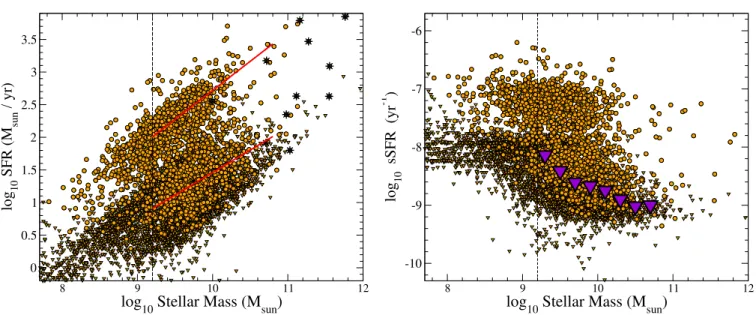
Figure 2 shows the resulting SFR and sSFR ver-sus stellar mass diagrams, which span more than three decades in stellar mass. In these plots we include the SFR and sSFR based on the derived Hα luminosities for the “Hα excess” galaxies and upper limits for all other galaxies at 3.9 ≤ z ≤ 4.9. These upper limits are based on the minimum line-complex EW that we can detect from flux excess in the 3.6 µm band. The vertical dashed lines indicate the 50% stellar-mass com-pleteness level of our sample, which is log10M∗≈ 9.2 at

3.9 ≤ z ≤ 4.9. Note that the 80% stellar-mass complete-ness level is log10M∗ ≈ 9.6, but no main conclusion in

this paper would change if we restricted our analysis to this higher stellar mass limit.

Caputi et al.

8 9 10 11 12

log₁₀ Stellar Mass (M_sun)

2 2.5 3 3.5 4 log 10 rest EW (H α +[NII]+[SII]) 8 9 10 11 12

log₁₀ Stellar Mass (M_sun)

0 0.2 0.4 0.6 0.8 1 Fraction of "H α excess" galaxies

AGN

contamination?

Figure 1. Left: (Hα + [NII] + [SII]) ((Hα + [NII]) at z > 4.8) rest EW versus stellar mass for the “Hα excess” galaxies at 3.9 ≤ z ≤ 4.9. The big purple circles show the median EW values at different stellar masses and the error bars indicate the two central quartiles of the EW distribution in each stellar mass bin. The vertical dashed line indicates the SMUVS 50% stellar-mass completeness at 3.9 ≤ z ≤ 4.9. Right: Fraction of SMUVS 3.9 ≤ z ≤ 4.9 galaxies with “Hα excess” versus stellar mass.

.

8 9 10 11 12

log

Stellar Mass (M

)

log

Stellar Mass (M

)

Figure 2. Left: SFR based on the derived Hα luminosities for “Hα excess” galaxies (circles) and upper limits derived for galaxies with no 3.6 µm excess (triangles), versus stellar mass, at 3.9 ≤ z ≤ 4.9. The asterisks indicate galaxies that are 24 µm detected, so they may have an AGN component in the IRAC bands. The “Hα excess” galaxies are clearly distributed in two clouds, which correspond to the galaxy main sequence and starbursts at those redshifts. The red lines show the results of linear regressions done on the two clouds separately, considering only galaxies with 9.2 ≤ log10(M∗) ≤ 10.8. Right: the corresponding

sSFR versus stellar mass diagram. The purple triangles indicate upper limits for the median sSFR per stellar mass bin, obtained considering all galaxies, i.e. the derived sSFR for “Hα excess” galaxies and upper limits for those with no 3.6 µm excess.

The asterisks on the SFR-M∗ _{plot indicate galaxies}

that have a 24 µm counterpart within a 2 arcsec ra-dius in the Mid Infrared Photometer for Spitzer (MIPS;

Rieke et al. 2004) S-COSMOS catalogue (Sanders et al. 2007). These sources correspond mostly to galaxies with log10(M∗) > 10.8. Given the limited depth of the 24 µm

catalogue, the detection of sources at 3.9 ≤ z ≤ 4.9 sug-gests that they are likely AGN. Unfortunately, an SED power-law analysis in the IRAC bands is not useful to study this issue further because of a k-correction effect: the maximum contribution of an AGN mid-IR power law is beyond the IRAC bands at such high redshifts, so

only the hottest dust AGN could be manifested as IR power-law sources in IRAC (Caputi 2013). But one of the 24 µm-detected most massive galaxies in our sample is indeed an X-ray source (Civano et al. 2016) spectro-scopically confirmed to be at z = 4.596, which indicates its AGN nature. Therefore, as a matter of precaution, we flagged the 24 µm detected sources in our sample and excluded all galaxies with log10(M∗) > 10.8 from

further analysis. This high fraction of 24 µm detections among the most massive “Hα excess” galaxies supports our AGN hypothesis also based on the reversing trend discussed in Section 4.1, which shows that the 3.6 µm incidence becomes higher at the highest mass end, after a continuous decrease from intermediate to high stellar masses.

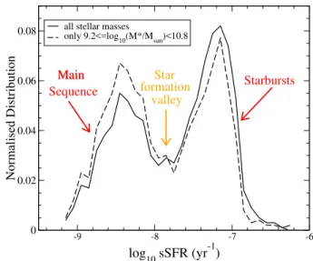
4.2.2. The bimodal distribution of Hα emitters on the SFR-M∗ plane

Fig.2 shows that the “Hα excess” galaxies form two distinct clouds on the SFR-M∗ and sSFR-M∗ planes. We identify these clouds as the so-called main-sequence of star formation (e.g.,Noeske et al. 2007; Rodighiero et al. 2010) and a starburst cloud, which appears to be more prominent than what is observed at any lower redshift. The two cloud separation becomes completely evident when we plot the fraction of “Hα excess” galax-ies versus sSFR (Fig. 3). From this Figure we can em-pirically derive that main-sequence galaxies are those with log10sSFR <_{∼ − 8.05, while starburst galaxies have}

log10sSFR >_{∼ − 7.60.}

In addition, there is an sSFR local minimum at −8.05 <_{∼ sSFR} <

∼ − 7.60 that here we denominate the star formation valley and likely contains galaxies in transition between the two star formation modes. This is analogous to the so-called ‘green valley’ which in the literature refers to galaxies in transition from the main sequence to the passive regime (e.g.,Balogh et al. 2011;

Zehavi et al. 2011;Renzini & Peng 2015).

On the sSFR-M∗ plot in Fig. 2 we indicate upper limits to the median sSFR per stellar mass bin, ob-tained from all the galaxies at 3.9 ≤ z ≤ 4.9. For the “Hα excess” galaxies we adopted the derived sSFR, while for the other galaxies we considered sSFR upper limits derived from the line complex EW (and corre-sponding Hα flux) upper limits. In that plot we clearly see that the upper limits to the median sSFR decrease with increasing stellar mass in the stellar mass range 9.2 ≤ log10(M∗) ≤ 10.8. This trend is consistent with

what is observed at lower z (e.g., Karim et al. 2011).

-9 -8 -7 -6 log 10 sSFR (yr -1 ) 0 0.02 0.04 0.06 0.08 Normalised Distribution

all stellar masses

only 9.2<=log₁₀(M*/M_sun)<10.8

Main Sequence Main _Starbursts formation valley Star

Figure 3. Normalised sSFR distribution of “Hα excess” galaxies at 3.9 ≤ z ≤ 4.9. The main sequence and starburst galaxies are clearly separated at these redshifts. Here we denominate ‘star formation valley’ to the region empirically determined to be at −8.05 ≤ log10(sSFR) ≤ −7.60. This is

analogous to the ‘green valley’ between the main sequence and passive regime, which is observed at lower redshifts.

We fitted the SFR-M∗ relation in the two clouds formed by the “Hα excess” galaxies in Fig.2(left) with simple linear regressions and obtained:

log10(SFR) = (0.69 ± 0.01) × log10(M∗) − (5.44 ± 0.13)

(2) for the main sequence and

log10(SFR) = (0.89±0.02)×log10(M∗)−(6.18+0.16_−0.15) (3)

for the starburst cloud. In these relations, we have obtained the error bars on the slopes and intercepts through Markov Chain Monte Carlo (MCMC) fittings, assuming a crude 30% average error on both the SFR and stellar mass.

The “Hα excess” galaxies identified as starbursts here constitute all the starbursts in our entire SMUVS sam-ple at 3.9 ≤ z ≤ 4.9, as virtually no SFR upper limit (corresponding to the non-“Hα excess” galaxies) lies on the starburst cloud in Fig. 2. Instead, the main se-quence defined by the “Hα excess” galaxies and fitted by Eq. (2) is not the complete main sequence at those redshifts. Therefore, we cannot use Eq. (2) along with analogous relations from the literature at lower redshifts to draw conclusions regarding the redshift evolution of the galaxy main sequence. Nonetheless, to put our re-sults in context, in Fig.4we show our separate main se-quence and starburst cloud fittings at z = 3.9−4.9, along

Caputi et al.

9 10 11 12

log

10 Stellar Mass (Msun) 0 0.5 1 1.5 2 2.5 3 3.5 log 10 SFR (M sun / yr) This work; z=3.9-4.9 S+14; z~4.3 S+14; z~2 W+14; z~2.25 B+18; z~2.5 Starbursts MS

Figure 4. Comparison of our “Hα excess” galaxy main sequence with main-sequence determinations from the liter-ature: S+14 (Speagle et al. 2014); W+14 (Whitaker et al. 2014) and B+18 (Bisigello et al. 2018), at different redshifts. Among these, only theBisigello et al. (2018) main-sequence has been obtained after a starburst segregation as we have performed here. We also show our starburst cloud fitting for reference.

with the median main-sequence determination by Spea-gle et al. (2014) at similar redshifts, which is given by log10(SFR) ≈ 0.80×log10(M∗)−6.36 at z ∼ 4.3. For

ref-erence, we also show some recent main-sequence deter-minations at 2 < z < 3 (Speagle et al. 2014;Whitaker et al. 2014; Bisigello et al. 2018). Among these lit-erature results, only the Bisigello et al. (2018) curve has been obtained after performing a starburst/main-sequence separation as we do here. The others fit all star-forming galaxies onto a single sequence.

The analysis of the different curves in Fig.4 tells us the following: firstly, the Speagle et al. (2014) main-sequence curve at z ∼ 4.3 is above our own, even when ours is an upper limit to the main-sequence which is biased for fitting only the “Hα excess” galaxies. This is simply because Speagle et al. (2014) do not sep-arate main sequence and starburst galaxies as we do, but rather fit a single relation for all star-forming galax-ies. Secondly, our “Hα excess” galaxy main sequence broadly coincides with the main sequences by Speagle et al. (2014) and Whitaker et al. (2014) at z ∼ 2. We caution the reader against a wrong interpretation: this coincidence is just fortuitous, as our own main-sequence is an upper limit and the Speagle et al. (2014) and

Whitaker et al. (2014) main sequences include all star-forming galaxies, so any direct comparison could be mis-leading. Our main-sequence determination can be more

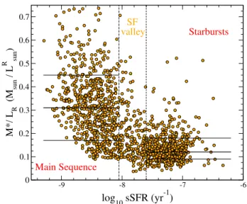
-9 -8 -7 -6 log 10 sSFR (yr -1 ) 0 0.1 0.2 0.3 0.4 0.5 0.6 0.7 M*/ L R (M sun / L R sun ) Starbursts Main Sequence SF valley

Figure 5. R-band mass-to-light ratios versus sSFR for our “Hα excess” galaxies with stellar mass 9.2 ≤ log10(M∗) ≤

10.8. The vertical lines indicate our empirical separation between main sequence and starburst galaxies, as well as the star-formation (SF) valley, according to their sSFR (see Fig 3). The horizontal lines in each of the main-sequence/starburst regions indicate the 16th, 50th and 84th percentiles of the M∗/LRdistributions.

fairly compared with that of Bisigello et al. (2018) at z ∼ 2.5, which has been obtained after a starburst segre-gation. Taking into account that our own main sequence at z = 3.9 − 4.9 is an upper limit to the true main se-quence at these redshifts, we can conclude that there is probably little or no evolution of this sequence between z ∼ 2.5 and z = 3.9 − 4.9.

4.2.3. The origin of the sSFR bimodality

A priori it may seem surprising that the bimodality displayed by the Hα emitters on the SFR-M∗and sSFR-M∗planes is not observed in the rest EW versus stellar mass diagram (Fig.1, left). Fumagalli et al. (2012) de-rived that the sSFR of an Hα emitter is proportional to the ratio between the line rest EW and the R-band mass-to-light ratio, i.e., sSFR ∝ EW/(M∗/LR), where

LR is the R-band luminosity. Therefore, one could

rea-sonably expect that the distribution of M∗/LRratios is

different for main sequence and starburst Hα emitters, and that this difference is to some extent responsible for the bimodal sSFR behaviour.

Figure 5 shows the R-band mass-to-light M∗/LR

ra-tio versus sSFR for our Hα emitters with stellar mass 9.2 ≤ log10(M∗) ≤ 10.8. The R-band luminosities LR

considered here correspond to continuum luminosities, and have been obtained from the best-fit templates in LEPHARE’s run excluding the 3.6 µm photometry.

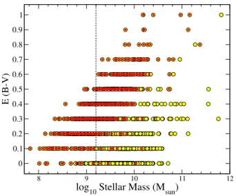
Al-8 9 10 11 12 log

10 Stellar Mass (Msun) 0 0.1 0.2 0.3 0.4 0.5 0.6 0.7 0.8 0.9 1 E (B-V)

Figure 6. Colour excess versus stellar mass for the “Hα excess” galaxies. Datapoints corresponding to our identified starbursts are highlighted with red dots. The vertical line indicates the SMUVS 50% stellar-mass completeness at 3.9 ≤ z ≤ 4.9.

though there is no bimodality in the M∗/LR ratios, a

decreasing trend of these values with increasing sSFR is evident, with starburst galaxies having a tight distribu-tion of small M∗/LRvalues. For the starbursts, we find

a median M∗/LR= 0.12, with 16th-84th percentiles of

0.09-0.18. Instead, main-sequence Hα emitters typically have larger M∗/LR, following a wide distribution: the

median is M∗/LR= 0.31 and the 16th-84th percentiles

are 0.17-0.45.

The small M∗/LR ratios for starbursts are mainly

the consequence of their systematic young ages, which typically are a few ×107_{yr, according to their best}

SED fitting templates. However, starbursts are not the only galaxies in our sample which are characterised by such young ages: about 20% of the “non-Hα excess” galaxies with stellar mass 9.2 ≤ log10(M∗) ≤ 10.8 at

3.9 ≤ z ≤ 4.9 have equally young best-fit ages in their SED fitting. Besides, starbursts are also characterised by having the largest extinction values among the “Hα excess” galaxies at fixed stellar mass, but there is no bi-modality in the colour excess E(B − V) distribution, as can be seen in Fig.6. All these facts indicate that the sSFR bimodality for the Hα emitters does not arise as a consequence of a single galaxy property, but is rather the consequence of the existence of a galaxy population (i.e., the starbursts) with a particular combination of properties: large Hα EW, young ages, and mostly high dust extinctions.

Although dust extinction and age can be degenerate in the SED fitting, this does not appear to be a

signif-icant problem for our starburst galaxies. If we analyze the probability density distribution as a function of age, marginalised over all other variables, we find that ∼90% of the starbursts have 84th percentiles at ages < 108yr, i.e., they are truly galaxies dominated by young stellar populations, in contrast to the main-sequence Hα emit-ters, whose ages are mostly > 108yr.

4.2.4. The importance of starburst galaxies at z ∼ 4 − 5

The existence of different regions on the SFR-M∗ plane, corresponding to different modes of star forma-tion, has been analyzed in the literature at different red-shifts, from the local Universe (Renzini & Peng 2015) to z ∼ 3 (e.g.,Santini et al. 2009;Kajisawa et al. 2010;

Wuyts et al. 2011; Ilbert et al. 2015). Here we show, for the first time, the existence of a prominent starburst sequence along with the main sequence on the SFR-M∗ plane at 3.9 ≤ z ≤ 4.9.

Starbursts constitute a small fraction (15%) of all the SMUVS galaxies at 3.9 ≤ z ≤ 4.9, but the percentage that we find here is significantly higher than the percent-ages found at z ∼ 2−3 (e.g.,Rodighiero et al. 2011; Sar-gent et al. 2012;Schreiber et al. 2015). This is the case in spite of defining starbursts with an sSFR cut which is quite higher than the value log10(sSFR) >_{∼ −8.1 adopted}

by Rodighiero et al. (2011) at z ∼ 2. At these lower redshifts, the percentage of galaxies with log10(M∗) > 9

and log10(sSFR) > −7.60 is negligible.

Starbursts and main-sequence galaxies are similarly important in number among our “Hα excess” galaxies with 9.2 ≤ log10(M∗) ≤ 10.8 at 3.9 ≤ z ≤ 4.9. However,

since starbursts make only ∼ 15% of all the SMUVS galaxies in these stellar mass and redshift bins, the me-dian sSFR upper limits shown in Fig.2(right) lie all on the star-formation main sequence.

Figure 7shows how the fraction of starburst galaxies at 3.9 ≤ z ≤ 4.9 varies with stellar mass. These frac-tions range from ∼ 0.25 at log10(M∗) ∼ 9.3 to < 0.05

at log10(M∗) > 10.2, showing that the starburst

phe-nomenon is much more common among intermediate-mass than intermediate-massive galaxies at z ∼ 4 − 5, consistently to what is predicted by theoretical galaxy models (e.g.,

Cowley et al. 2017) and observed at lower redshifts (e.g.,

Bisigello et al. 2018).

It is interesting to do a back-of-the-envelope calcu-lation of how much stellar mass these starbursts could accumulate at these redshifts. A log10(sSFR) = −7.2

value implies a stellar-mass doubling time of 1/sSFR ≈ 1.6 × 107_{yr = 0.016 Gyr. The elapsed time between z =}

4.9 and z = 3.9 is 0.379 Gyr. Besides, from Fig.7we see that the fraction of galaxies with log10(M∗) ∼ 9.5 that

Caputi et al.

9 10 11

log

10 Stellar mass (Msun) 0 0.05 0.1 0.15 0.2 0.25 Starburst Fraction

Figure 7. Fraction of starbursts (defined as galaxies with log10(sSFR) > −7.60) in different stellar mass bins among

all the SMUVS galaxies at 3.9 ≤ z ≤ 4.9.

with similar stellar mass would spend a similar amount of time in the starburst phase, then the log10(M∗) ∼ 9.5

galaxies would spend a fifth of the above-mentioned elapsed time as starbursts, i.e., ∼ 0.076 Gyr, which is almost five times the stellar-mass doubling time. There-fore, assuming a recycled fraction of 50%, we infer that these galaxies could grow their stellar mass by a factor of ∼ 2.5 at those redshifts. This means that a typical M∗ ∼ 3 × 109_M

 galaxy at 3.9 ≤ z ≤ 4.9 would

be-come a galaxy with M∗ ∼ 8 × 109_M

 at z < 3.9. This

crude estimate shows that the large sSFR values derived here are consistent with a rapid, but plausible, growth of intermediate-mass galaxies happening ∼ 1.5 Gyr after the Big Bang.

4.3. The inferred cosmic star formation rate density at z = 3.9 − 4.9

We can use our derived SFR to obtain an estimate of the cosmic SFR density (SFRD) at 3.9 ≤ z ≤ 4.9. Considering only the “Hα excess” galaxies gives us a lower limit to the SFRD. Instead, if we added the SFR contributions of all the other SMUVS galaxies at these redshifts, for which we only have SFR upper limits, we could estimate an upper limit to the SFRD. However, we recall that SMUVS significantly loses completeness at stellar masses log10(M∗) < 9.2, so even if we apply

completeness corrections, we can only extrapolate the missing galaxy SFRs based on the galaxies that we de-tect. Therefore, estimating a more secure upper limit requires accounting somehow for the galaxies that we do not see. This can be done, at least in a crude man-ner, taking into account the faint-end slope of the galaxy

stellar mass function (GSMF) at those redshifts and as-suming that the SFR versus stellar mass trends shown in Fig.2can be extrapolated to lower stellar masses.

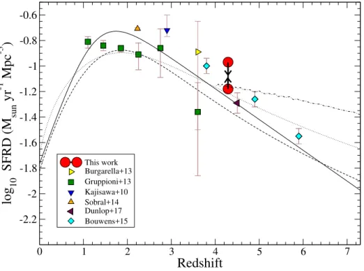
Figure 8shows the redshift evolution of the SFRD in the so-called Lilly-Madau diagram (Lilly et al. 1996;

Madau et al. 1996). In this plot we have included our derived lower and upper limits to the SFRD at a median redshift hzi = 4.29, as well as a compilation of values re-cently reported in the literature, which are based on dif-ferent galaxy surveys and individual galaxy SFRs from a variety of SFR tracers: UV fluxes (Bouwens et al. 2015); spectral line emission from narrow-band surveys (Sobral et al. 2014); far-IR fluxes (Gruppioni et al. 2013); and a combination of UV and IR fluxes (Kajisawa et al. 2010;

Burgarella et al. 2013; Dunlop et al. 2017). Multiple other previous works have presented SFRD estimates at high z, especially based on UV fluxes. However, UV-based SFRs are much more affected by dust-extinction corrections than those based on any other tracer, mak-ing the resultmak-ing SFRD values particularly uncertain at least to z ∼ 6 (see e.g.,Castellano et al. 2014).

In the derivation of our own SFRD, we have explic-itly excluded all galaxies with log10(M∗) > 10.8 to

minimize any plausible AGN contamination (see dis-cussion in Section 4.2). By considering only the SFR of “Hα excess” galaxies we obtained a robust SFRD lower limit of 0.066 Myr−1Mpc−3. To obtain an

SFRD upper limit, we estimated separately the contri-butions of all galaxies with 9.2 ≤ log10M∗ ≤ 10.8 and

8 ≤ log10M∗ < 9.2 and added them up, as follows. For

the 9.2 ≤ log10M∗ ≤ 10.8 objects we directly adopted

our derived SFR (“Hα excess” galaxies) or SFR upper limits (for the other galaxies). To account for the con-tribution of lower mass galaxies we considered that the extrapolation of the GSMF at z = 4 − 5 (Caputi et al. 2015;Grazian et al. 2015) indicates that we should ex-pect ∼ 5 times more galaxies with 8 ≤ log10M∗ < 9.2

than with log10M∗ ≥ 9.2. And according to Fig. 2,

the 8 ≤ log10M∗ < 9.2 objects should have on

av-erage SFR that are about a dex lower than the more massive galaxies. Thus, the lower mass galaxies should roughly add ∼ 50% to the SFRD value calculated based only on the 9.2 ≤ log10M∗ ≤ 10.8 sources. With all

these considerations, we obtain an SFRD upper limit of 0.106 Myr−1Mpc−3. All the SFRD quoted here and in

Fig.8correspond to aSalpeter (1955) IMF over stellar masses (0.1 − 100) M to facilitate the comparison with

the literature, in which this IMF is mostly used. Our resulting range of SFRD at hzi = 4.29 is in good agree-ment with the other recent observational determinations in the literature.

0 1 2 3 4 5 6 7

Redshift

log

SFRD (M

yr

Mpc

)

Figure 8. Cosmic star formation rate density versus redshift. The large red circles at z = 4.29 indicate our own lower and upper limit determinations. To derive the SFRD lower limit, we considered only the SFR of “Hα excess” galaxies with log10(M∗) ≤ 10.8. To derive the upper limit, we took into account the SFR of all SMUVS galaxies with 9.2 ≤ log10(M∗) ≤ 10.8

at 3.9 ≤ z ≤ 4.9 (exact values for the “Hα excess” galaxies and upper limits for all the others), and applied a correction factor for lower stellar masses inferred from the GSMF extrapolation at those redshifts (see text). In both cases, only galaxies with log10(M∗) ≤ 10.8 have been taken into account to minimize any possible AGN contamination. Other symbols show recent SFRD

determinations from the literature, based on different SFR tracers. The different curves correspond to either data-compilation best fits or theoretical predictions from the literature. Solid line: Behroozi et al. (2013); dashed-dotted line: Dayal et al. (2014); dashed line: Madau & Dickinson (2014); dotted line: Khaire & Srianand (2014). All SFRD values in this figure correspond to aSalpeter (1955) IMF over stellar masses (0.1 − 100) M. This is the only figure in this paper in which this IMF is adopted,

only for the purpose of facilitating the comparison with the literature.

The different curves in Fig.8 show best fits to com-pilations of observational data (Behroozi et al. 2013;

Madau & Dickinson 2014) and theoretical predictions (Dayal et al. 2014; Khaire & Srianand 2014). We see that the majority of the most recent SFRD estimates at high z, including our own, are at least 0.10-0.15 dex above the best fits provided by Madau & Dickinson

(2014) and Behroozi et al. (2013). This is probably because most of the observational works considered for these fits calculated SFRs based on UV fluxes, which are very sensitive to dust extinction corrections, as men-tioned above. A revision of these corrections (Bouwens et al. 2015) or, even better, a consideration of UV+IR data (Kajisawa et al. 2010; Burgarella et al. 2013) or SFRs based on line emission like those we obtain here should provide better constraints to the cosmic SFRDs at high z at least to z ∼ 6. Dust extinction corrections are expected to be less critical at earlier cosmic times, but this will have to be confirmed in the future, with

systematic IR galaxy surveys that can trace Balmer line emission in the early Universe, which will happen with the James Webb Space Telescope (JWST). The theoreti-cal predictions appear to be in good agreement with our SFRD lower limit at hzi = 4.29, as well as some of the other observational data points.

The contribution of starburst galaxies to the total SFRD budget up to z ∼ 3 has been discussed in the literature (e.g., Rodighiero et al. 2011; Sargent et al. 2012;Schreiber et al. 2015). The derived contributions vary according to the selection effects and the starburst definition adopted by different groups, but in all cases it has been found that starbursts make <_{∼ 15% of the} total SFRD. As we discussed before, all these studies have been based on the analysis of M∗ >_{∼ 10}10_M

galax-ies. Here, we obtain that the “Hα excess” galaxies de-fined as starbursts by log10(sSFR) >_{∼ − 7.60 account for}

> 50% of our upper limit to the SFRD (and 84% of our lower limit based only on the “Hα excess” galaxies)

Caputi et al. at 3.9 ≤ z ≤ 4.9. These percentages are substantially

higher than all previous determinations. The key reason for this higher percentage is that here we are including galaxies down to lower stellar masses, which are much more numerous than massive galaxies and have a higher fraction of starbursts among them.

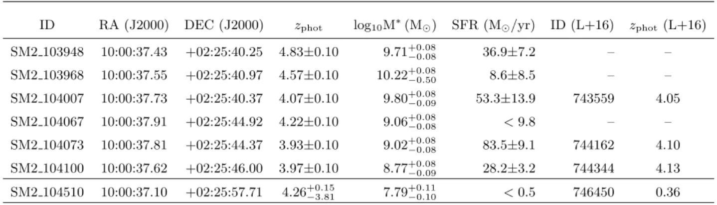
4.4. A > 50σ overdensity of 3.9 ≤ z ≤ 4.9 galaxies Within our analysis of SMUVS galaxies at 3.9 ≤ z ≤ 4.9, we find that six of these sources lie in a very small region of only ∼ 0.20 × 0.20 arcmin2, with a median redshift z ≈ 4.2. We have a total of 5925 SMUVS galaxies at those redshifts over a total area of 0.66 deg2, which makes for an average surface density of ∼2.5 arcmin−2_{. Therefore, the six galaxies concentrated}

in the tiny ∼ 0.20 × 0.20 arcmin2 _{area constitute a}

re-markable > 50σ overdensity of sources at 3.9 ≤ z ≤ 4.9. Figure 9 shows the UltraVISTA HKs stack and SMUVS 3.6 µm images of this galaxy overdensity. The properties of the six individual galaxies, as well as those of another galaxy at a similar (albeit less secure) red-shift, which lies only ∼0.3 arcmin apart, are given in Table1.

In the main overdensity region, three out of six galax-ies have redshifts 3.93 ≤ z ≤ 4.07. Within the error bars, this suggests that these galaxies are likely part of the same bound structure. These three galaxies are also present in the COSMOS2015 catalogue byLaigle et al.

(2016), whose photometry and redshifts have been in-dependently determined based on a previous release of the UltraVISTA data (DR2) and shallower Spitzer data (see Table 1). Their photometric redshifts are consis-tent with ours within the error bars. These independent results support our claim that a z ∼ 4 overdensity is present in that region of the sky. The other three galax-ies that we find in the overdesity region are at higher redshifts 4.22 ≤ z ≤ 4.83, so spectroscopic data are needed to determine whether they belong to the same structure or not.

Among the six galaxies in the overdensity, five are classified as “Hα excess” sources, although for one of them this classification is marginal. The other four have SFRs corresponding to several tens M/yr. Note,

how-ever, that only one of them (ID SM2 104073) is a star-burst galaxy, while the others are main sequence galax-ies. All these galaxies have intermediate stellar masses, with only one of them having log10M∗> 10.

5. DISCUSSION AND CONCLUSIONS

In this paper we have studied a sample of 5925 galaxies at 3.9 ≤ z ≤ 4.9 from the SMUVS survey over 0.66 deg2

of the COSMOS field. We have analyzed the presence

of flux excess in the IRAC 3.6 µm band to identify “Hα excess” galaxies at these redshifts. From the inferred Hα EW we have derived SFR and sSFR for these galaxies and obtain upper limits for all the other galaxies at these redshifts.

The incidence of “Hα excess” galaxies in our 3.9 ≤ z ≤ 4.9 sample decreases from stellar masses log10(M∗) ∼ 9.2

through log10(M∗) ∼ 10.8, indicating that intense

star formation is relatively more important among intermediate-mass than massive galaxies at these red-shifts. At higher stellar masses, surprisingly, we see a reversing trend which seems difficult to explain by simply invoking enhanced star formation for the most massive systems. As a large fraction of the most mas-sive galaxies with 3.6 µm flux excess at 3.9 ≤ z ≤ 4.9 are 24 µm-detected, we suggest that AGN activity could at least be partly responsible for this flux excess. This statement is supported by a spectroscopically confirmed AGN among the most massive “Hα excess” galaxies.

The most important result in this paper is that we found that the “Hα excess” galaxies form two distinct sequences on the SFR-M∗ plane, which we recognise as the so-called formation main sequence and a star-burst sequence. Although the exact location of galaxies on these planes depends on the SED fitting assumptions, we have shown that the sSFR bimodality is indepen-dent of the assumed metallicities and dust reddening law, under reasonable assumptions. Starburst galaxies are characterised by a unique combination of large Hα EW, young ages and mostly high dust extinctions, which result in very high sSFR.

This suggests the existence of two distinct star for-mation modes, one corresponding to secular baryonic accretion within dark matter haloes (giving rise to the main sequence), and another one much more effective for rapid galaxy growth, possibly linked to galaxy merg-ers or external perturbations that produce the starburst phase. A fundamental intrinsic assumption in all these results is that the same conversion from gas into stars given by Kennicutt’s law (equation1) is valid for all star-forming galaxies at high z. Demonstrating this general validity is extremely difficult, but recent studies of the link between gas content and star formation in high-z galaxies suggest that a universal conversion may indeed hold (e.g., Scoville et al. 2016).

The star-formation main sequence at different red-shifts has been analyzed from multiple observational datasets (e.g., Brinchmann et al. 2004; Noeske et al. 2007;Rodighiero et al. 2010;Elbaz et al. 2011;Speagle et al. 2014; Whitaker et al. 2014; Tasca et al. 2015). Theoretical studies have attempted to explain the main sequence as a mere consequence of gas accretion within

Figure 9. A > 50σ overdensity of SMUVS galaxies at z ≈ 4.2. Left: UltraVISTA HKs mosaic; right: SMUVS 3.6 µm

mosaic. In addition to the six galaxies making the unusually high overdensity, a seventh galaxy with similar redshift is present only ∼ 0.3 arcmin apart. The properties of individual galaxies are listed in Table 1. Each image corresponds to an area of ∼ 0.8 × 0.8 arcmin2

.

dark matter haloes (e.g., Somerville et al. 2008;Lu et al. 2014;Cousin et al. 2015), but have difficulty in re-producing the evolution of its normalization with cosmic time (Dutton et al. 2010; Gennel et al. 2014;Furlong et al. 2015; Sparre et al. 2015) – seeMitchell et al.

(2014) for a thorough discussion of this problem. Other groups have investigated the role of galaxy-black hole co-evolution in shaping the star formation main sequence (e.g.,Mancuso et al. 2016;Kaviraj et al. 2017). In any case, a complete theoretical explanation of this relation between stellar mass and instantaneous star formation rate is still missing.

In contrast to the widely discussed main sequence, most observational studies have failed to recognise the presence of a separate starburst cloud on the SFR-M∗ plane (its existence has been suggested byCassar`a et al.

(2016), but these authors referred to it as a “second main sequence”). The failure to recognise the starburst cloud is mainly due to the relatively small galaxy samples an-alyzed in most of the literature, with starburst galax-ies typically identified and studied only among mas-sive galaxies (Rodighiero et al. 2011; Sargent et al. 2012). Here we show, for the first time, that star-burst galaxies make a clearly distinct sequence on the SFR-M∗ plane and constitute a significant percentage (∼ 15%) of all galaxies with 9.2 ≤ log10M∗ ≤ 10.8 at

3.9 ≤ z ≤ 4.9. Only a slightly smaller percentage is obtained at z ∼ 2 − 3 when a broad dynamic range in stellar mass is considered, albeit with significantly lower sSFR (Bisigello et al. 2018). We find that the fraction of starburst galaxies has a strong dependence on stel-lar mass, varying between ∼ 0.25 at log10(M∗) ∼ 9.3

to < 0.05 at log10(M∗) > 10.2. This is also expected

from galaxy formation models (e.g.,Vogelsberger et al. 2014).

The starburst galaxies in our sample are charac-terised by log10(sSFR) > −7.60. At redshifts z <_{∼ 4,}

these very high sSFR values are very unusual and have only been found to be common among low stellar-mass M∗<

∼ 108Myoung galaxies – see, e.g., Fig. 11 in

Kar-man et al. (2017), and also Amor´ın et al. (2017);

Vanzella et al. (2017). Here we show that these high sSFRs are relatively common among star forming, intermediate-mass galaxies at 3.9 ≤ z ≤ 4.9.

Another key result of this paper is that starbursts make for at least 50% of the total SFRD budget at z ∼ 4 − 5. This percentage is substantially higher than any previous determination found in the literature. This is because previous starburst studies only analyzed galaxies with M∗ >_{∼ 10}10_M

 (up to z ∼ 3). The

inclu-sion of lower mass galaxies is essential to recognise the importance of the starburst phase and how much it con-tributes to the total cosmic SFRD, particularly at high redshifts.

We have also discovered an unusually high-significance galaxy overdensity at these high redshifts. A total of six galaxies in our high-z sample reside in a tiny area of 0.20 × 0.20 arcmin2_{, five of which correspond to “Hα}

ex-cess” sources. The spectroscopic confirmation of such an overdensity would unveil one of the most concentrated active sites of star formation known at z ∼ 4 − 5.

All the results presented in this paper have exploited the unique combination of area and depth provided by the SMUVS survey at mid-IR wavelengths. This survey has provided us with an unprecedented level of statis-tics and dynamic range which are fundamental to reveal

Caputi et al.

Table 1. Properties of individual sources in the z ≈ 4.2 galaxy overdensity.

ID RA (J2000) DEC (J2000) zphot log10M∗(M) SFR (M/yr) ID (L+16) zphot(L+16)

SM2 103948 10:00:37.43 +02:25:40.25 4.83±0.10 9.71+0.08 −0.08 36.9±7.2 – – SM2 103968 10:00:37.55 +02:25:40.97 4.57±0.10 10.22+0.08−0.50 8.6±8.5 – – SM2 104007 10:00:37.73 +02:25:40.37 4.07±0.10 9.80+0.08−0.09 53.3±13.9 743559 4.05 SM2 104067 10:00:37.91 +02:25:44.92 4.22±0.10 9.06+0.08 −0.08 < 9.8 – – SM2 104073 10:00:37.81 +02:25:44.37 3.93±0.10 9.02+0.08−0.08 83.5±9.1 744162 4.10 SM2 104100 10:00:37.62 +02:25:46.00 3.97±0.10 8.77+0.08−0.09 28.2±3.2 744344 4.13 SM2 104510 10:00:37.10 +02:25:57.71 4.26+0.15−3.81 7.79 +0.11 −0.10 < 0.5 746450 0.36

Note—Source coordinates correspond to the HKs mosaic. The SFR values are based on the inferred Hα rest EWs and fluxes

derived from the 3.6 µm photometry. The last two columns contain ID and photometric redshifts from the COSMOS 2015 catalogue by Laigle et al. (2016; L+16). The last row corresponds to a galaxy outside the main overdensity region, but only ∼ 0.3 arcmin apart from it.

unknown aspects of galaxy evolution in the young Uni-verse.

Based in part on observations carried out with the Spitzer Space Telescope, which is operated by the Jet Propulsion Laboratory, California Institute of Technol-ogy under a contract with NASA. Also based on data products from observations conducted with ESO Tele-scopes at the Paranal Observatory under ESO program ID 179.A-2005 and on data products produced by TER-APIX and the Cambridge Astronomy Survey Unit on behalf of the UltraVISTA consortium. Also based on observations carried out by NASA/ESA Hubble Space

Telescope, obtained and archived at the Space Telescope Science Institute; and the Subaru Telescope, which is operated by the National Astronomical Observatory of Japan. This research has made use of the NASA/IPAC Infrared Science Archive, which is operated by the Jet Propulsion Laboratory, California Institute of Technol-ogy, under contract with NASA.

We thank an anonymous referee for a constructive re-port. KIC, SD and WC acknowledge funding from the European Research Council through the award of the Consolidator Grant ID 681627-BUILDUP.

Facilities:

Software:

APPENDIX

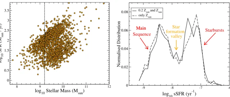
A. IMPACT OF CONSIDERING TWO METALLICITIES FOR THE Hα EXCESS GALAXIES

8 9 10 11 12

log

Stellar Mass (M

)

log

sSFR (yr

)

0.2 Z_sun and Z_sun only Z_sun Main Sequence Main _Starbursts formation valley Star

Figure 10. Left: SFR based on the derived Hα luminosities for “Hα excess” galaxies versus stellar mass at 3.9 ≤ z ≤ 4.9, obtained after allowing for two possible metallicities (Zand 0.2 Z) in the SED fitting. Right: resulting sSFR distribution for

the “Hα excess” galaxies with 9.2 ≤ log10(M∗) ≤ 10.8.

In this paper we have modelled the SEDs of our 3.9 ≤ z ≤ 4.9 galaxies assuming a solar metallicity. Other authors have preferred to adopt a much lower metallicity (0.2 Z) to study “Hα excess” galaxies at similar redshifts (e.g.,Smit

et al. 2016). However, in a stellar-mass selected galaxy sample like SMUVS, the adoption of sub-sollar metallicities for all galaxies is likely not correct (e.g. Scoville et al. 2016). The most likely scenario is that our galaxies span a range of metallicities between a fraction of the solar and the entire solar values.

To test the impact of this effect on our results, we have re-run the SED fitting of our “Hα excess” galaxies at 3.9 ≤ z ≤ 4.9 allowing LePhare to use both templates with 0.2 Z and Z metallicities, covering the same grid for all

the other parameter values (i.e., star formation histories, ages, extinctions). By doing this, we found that: i) 96% of all our original “Hα excess” galaxies are confirmed to be in the redshift range 3.9 ≤ z ≤ 4.9, and thus confirmed as Hα emitting sources; ii) about 34% of the original “Hα excess” galaxies have a best-fit SED with 0.2 Z, while ∼ 62%

Caputi et al.

Taking into account these results, we re-computed the Hα rest EW and fluxes for the “Hα excess” galaxies that have a best-fit SED with 0.2 Z in the new LePhare run. At this low metallicity, the net Hα contribution to the

total 3.6 µm flux excess is given by (Anders & Fritze-van Alvensleben 2003): f (Hα)= 0.81f (Hα + [NII] + [SII]) and f (Hα)= 0.92f (Hα + [NII]), which are valid at 3.9 ≤ z ≤ 4.8 and 4.8 < z ≤ 4.9, respectively. Finally, we derived the corresponding clean Hα luminosities and SFR in the same way as explained in Section §4.2.

Figure10 (left) shows the resulting SFR-M∗ plane for “Hα excess” galaxies when considering two metallicities for the SED fitting (we only plotted here the 96% of the original “Hα excess” sources that stayed in the 3.9 ≤ z ≤ 4.9 redshift range in the new SED-fitting run). Qualitatively, this plot looks similar to the analogous plot in Fig. 2, with two distinct galaxy star-formation main sequence and starburst cloud clearly visible. Fig. 10(right) shows the corresponding sSFR distribution compared to the original distribution derived adopting only solar metallicity (see Fig.3). This plot confirms the existence of two sSFR regimes, separated by a star formation valley corresponding to an underdensity of sources with −8.05 <_{∼ sSFR} <

∼ − 7.60. Therefore, we can conclude that all the main results in this paper are robust against our SED metallicity assumptions.

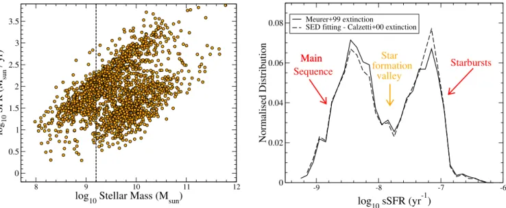
B. IMPACT OF CONSIDERING A REDDENING LAW DEPENDENT ON THE UV SLOPE β

Another parameter that could potentially influence our results is the choice of dust reddening law in the SED fitting and recovery of intrinsic Hα luminosities. In this work we have adopted theCalzetti et al. (2000) reddening law for the SED fitting and applied the derived colour excess from the best-fit SED of each “Hα excess” galaxy to determine its intrinsic Hα flux. Here we investigate the impact of a different assumption, namely, that the internal extinction of each galaxy is directly related to its UV spectral slope β, which is defined as the slope in fλ(λ) ∝ λβ for rest-frame

1500 < λ < 2500 ˚A.

8 9 10 11 12

log₁₀ Stellar Mass (M_sun)

0 0.5 1 1.5 2 2.5 3 3.5 log 10 SFR (M sun / yr) -9 -8 -7 -6 log 10 sSFR (yr -1 ) 0 0.02 0.04 0.06 0.08 Normalised Distribution Meurer+99 extinction

SED fitting - Calzetti+00 extinction

Main Sequence Main _Starbursts formation valley Star

Figure 11. Left: SFR based on the derived Hα luminosities for “Hα excess” galaxies versus stellar mass at 3.9 ≤ z ≤ 4.9, obtained after considering a dust extinction correction dependent on the rest UV slope of each galaxy, following theMeurer et al. (1999) relation. Right: resulting sSFR distribution for the “Hα excess” galaxies with 9.2 ≤ log10(M∗) ≤ 10.8.

We computed the UV slope β of each of our galaxies by fitting this power-law functional form to the photometric fluxes tracing rest 1500 < λ < 2500 ˚A, which correspond to about ten photometric bands in the COSMOS field (as has been done by e.g.,Fudamoto et al. 2017). Then we assumed that the internal dust extinction was given by the

Meurer et al. (1999) law: A1600 = 4.43 + 1.99β, and considered a conversion A6563 ≈ A1600/3.2. We applied this

new extinction correction (which we considered to be the same for the continuum and line) to each galaxy, and we re-computed its Hα rest EW and luminosity, and derived the corresponding SFR.

Fig.11is the analogue of Fig.10, but in this case we show the SFR-M∗plane and sSFR distribution that result from considering the new dust extinction correction (at fixed solar metallicity, as in Section 4). The star-formation main sequence and starburst cloud are clearly distinct in these plots, showing that the sSFR bimodality is still present when

we consider a single, β-dependent extinction relation rather than the best-fit extinction obtained from the individual SED fitting of each of our galaxies. We conclude that the observed sSFR bimodality is robust to reasonable changes in the modelling assumptions.

REFERENCES

Amor´ın, R., Fontana, A., P´erez-Montero, E. et al., 2017, NatAs, 1E, 52

Anders, P., Fritze-van Alvensleben, U., 2003, A&A, 401, 1063

Arnouts, S., Cristiani, S., Moscardini, L. et al., 1999, MNRAS, 310, 540

Ashby, M. L. N., Willner, S. P., Fazio, G. G. et al., 2013, ApJ, 769, 80

Ashby, M. L. N., Willner, S. P., Fazio, G. G. et al., 2015, ApJS, 218, 33

Balogh, M. L., McGee, S. L., Wilman, D.J. et al., 2011, MNRAS, 412, 2303

Behroozi, P. S., Wechsler, R. H., Conroy, C., 2013, ApJ, 770, 57

Bertin, E., & Arnouts, S. 1996, A&AS, 117, 393 Bisigello, L., Caputi, K. I., Grogin, N., Koekemoer, A.,

2018, A&A, submitted (arXiv:1706.06154)

Bouwens, R. J., Illingworth, G. D., Oesch, P. A. et al., 2015, ApJ, 803, 34

Brinchmann, J., Charlot, S., White, S. D. M. et al., 2004, MNRAS, 351, 1151

Bruzual, G., Charlot, S., 2003, MNRAS, 344, 1000 Burgarella, D., Buat, V., Gruppioni, C. et al., 2013, A&A,

554, A70

Calzetti, D., Armus, L., Bohlin, R. C. et al., 2000, ApJ, 533, 682

Caputi, K. I., Cirasuolo, M., Dunlop J. S. et al., 2011, MNRAS, 413, 162

Caputi, K. I., 2013, ApJ, 768, 103

Caputi, K. I., Ilbert, O., Laigle, C. et al., 2015, ApJ, 810, 73 Cassar`a, L. P., Maccagni, D., Garilli, B. et al., 2016, A&A,

593, A9

Castellano, M., Sommariva, V., Fontana, A. et al., 2014, A&A, 566, A19

Chabrier, G., 2003, PASP, 115, 763

Civano, F., Marchesi, S., Comastri, A. et al., 2016, ApJ, 819, 62

Cousin, M., Lagache, G., B´ethermin, M. et al., A&A, 575, A32

Cowley, W. I., B´ethermin, M., Lagos, C. del P. et al., 2017, MNRAS, 467, 1231

Dayal, P., Ferrara, A., Dunlop, J. S., Pacucci, F., 2014, MNRAS, 445, 2545

Dutton, A. A., van den Bosch, F. C., Dekel, A., 2010, MNRAS, 405, 1690

Dunlop, J. S., McLure, R. J., Biggs, A. D. et al., MNRAS, 466, 861

Elbaz, D., Dickinson, M., Hwang, H. S. et al., 2011, A&A, 533, A119

Faisst, A. L., Capak, P., Hsieh, B. C. et al., 2016, ApJ, 821, 122

Fazio, G. G., Hora, J. L., Allen, L. E. et al., 2004, ApJS, 154, 10

Fudamoto, Y, Oesch, P. A., Schinnerer, E. et al., 2017, MNRAS, submitted (arXiv:1705.01559)

Fumagalli, M., Patel, S. G., Franx, M. et al., 2012, ApJ, 757, L22

Furlong, M., Bower, R. G., Theuns, T. et al., 2015, MNRAS, 450, 4486

Genel, S., Vogelsberger, M., Springel, V. et al., 2014, MNRAS, 445, 175

Grazian, A., Fontana, A., Santini, P. et al., 2015, A&A, 575A, 96

Gruppioni, C., Pozzi, F., Rodighiero, G. et al., 2013, MNRAS, 432, 23

Hopkins, A. M., Beacom, J. F., 2006, ApJ, 651, 142 Ilbert, O., Arnouts, S., McCracken, H. J. et al., 2006, A&A,

457, 8415

Ilbert, O., Arnouts, S., Le Floc’h, E. et al., 2015, A&A, 579, A2

Kajisawa, M., Ichikawa, T., yamada, T. et al., 2010, ApJ, 723, 129

Karim, A., Schinnerer, E., Mart´ınez-Sansigre, A. et al., ApJ, 730, 61

Karman, W., Caputi, K. I., Caminha, G. B. et al., 2017, A&A, 599, A28

Kaviraj, S., Laigle, C., Kimm, T. et al., 2017, MNRAS, 467, 4739

Kennicutt, R. C. Jr., 1998, ARA&A, 36, 189 Khaire, V., Srianand, R., 2015, ApJ, 805, 33 Lagos, C. del P., Theuns, T., Schaye, J. et al., 2016,

MNRAS, 459, 2632

Laigle, C., McCracken, H. J., Ilbert, O. et al., 2016, ApJS, 224, 24

Lilly, S. J., Le F`evre, O., Hammer, F., Crampton, O., 1996, ApJ, 460, L1

Caputi et al.

Lilly, S. J., Le F`evre, O., Renzini, A. et al., 2007, ApJS, 172, 70

Lu, Y., Wechsler, R. H., Somerville, R. S. et al., 2014, ApJ, 795, 123

Madau, P., Ferguson, H. C., Dickinson, M. E. et al., 1996, MNRAS, 283, 1388

Madau, P., Dickinson, M., 2014, ARA&A, 52, 415 Mancuso, C., Lapi, A., Shi, J. et al., 2016, ApJ, 833, 152 M´armol-Queralt´o , E., McLure, R. J., Cullen, F. et al.,

2016, MNRAS, 460, 3587

McCracken, H. J., Milvang-Jensen, B., Dunlop, J. et al., 2012, A&A, 544, A156

Meurer, G. R., Heckmann, T., Calzetti, D., 1999. ApJ, 521, 64

Mitchell, P. D., Lacey, C. G., Cole, S., Baugh, C. M., 2014, MNRAS, 444, 2637

Mouhcine, M., Lewis, I, Jones, B. et al., 2005, MNRAS, 362, 1143

Noeske, K. G., Weiner, B. J., Faber, S. M. et al., 2007, ApJ, 660, L43

Oke, J. B., Gunn, J. E., 1983, ApJ, 266, 713

Popping, G., Caputi, K. I., Trager, S. C. et al., 2015, MNRAS, 454, 2258

Reddy, N., Erb, D. K., Pettini, M. et al., 2010, ApJ, 712, 1070

Renzini, A., Peng, Y., 2015, ApJ, 801, L29

Rieke, G. H., Young, E. T., Engelbracht, C. W. et al., 2004, ApJS, 154, 25

Rodighiero, G., Cimatti, A., Gruppioni, C. et al, 2010, A&A, 518, L25

Rodighiero, G., Daddi, E., Baronchelli, I. et al., 2011, ApJ, 739, L40

Rodighiero, G., Renzini, A., Daddi, E. et al., 2014, MNRAS, 443, 19

Salpeter, E. E., 1955, ApJ, 121, 161

Sanders, D.B., Salvato, M., Aussel, H. et al., 2007, ApJS, 172, 86

Santini, P., Fontana, A., Grazian, A. et al., 2009, A&A, 504, 751

Sargent, M., B´ethermin, M., Daddi, E., Elbaz, D., 2012, ApJ, 747, L31

Schreiber, C., Pannella, M., Elbaz, D. et al., 2015, A&A, 575, A74

Scoville, N., Aussel, H., Brusa, M. et al., 2007, ApJS, 172, 1 Scoville, N., Sheth, K., Aussel, H. et al., 2016, ApJ, 820, 83 Shim, H., Chary, R.-R., Dickinson, M. et al., 2011, ApJ,

738, 69

Shivaei, I., Reddy, N. A. , Shapley, A. E. et al., 2015, ApJ, 815, 98

Smit, R., Bouwens, R. J., Labb´e, I. et al., 2016, ApJ, 833, 254

Sobral, D., Best, P. N., Smail, I. et al., 2014, MNRAS, 437, 3516

Somerville, R. S., Hopkins, P. F., Cox, T. J. et al., 2008, MNRAS, 391, 481

Sparre, M., Hayward, C. C., Springel, V. et al., 2015, MNRAS, 447, 3548

Speagle, J. S., Steinhardt, C. L., Capak, P. L., Silverman, J. D., 2014, ApJS, 214, 15

Stark, D. P., Schenker, M. A., Ellis, R. et al., 2013, ApJ, 763, 129

Steinhardt, C. L., Speagle, J. S., Capak, P. et al., 2014, ApJ, 791, L25

Taniguchi, Y., Scoville, N., Murayama, T. et al., 2007, ApJS, 172, 9

Tasca, L. A. M., Le F`evre, O., Hathi, N. P. et al., 2015, A&A, 581, A54

Vanzella, E., Calura, F., Meneghetti, F. et al., 2017, MNRAS, 467, 4304

Vogelsberger, M., Genel, S., Springel, V. et al., 2015, MNRAS, 444, 1518

Werner M. W., Roellig, T. L., Low, F. J. et al., 2004, ApJS, 154, 1

Whitaker, K. E., Franx, M., Leja, J. et al., 2014, ApJ, 795, 104

Wuyts. S., F¨orster-Schreiber, N., van der Wel, A. et al., 2011, ApJ, 742, 96

Zehavi, I., Zheng, Z., Weinberg, D. H. et al., 2007, ApJ, 736, 59