Mean-field theory of localization in a fuse model

HAL Id: hal-00107354

https://hal.archives-ouvertes.fr/hal-00107354

Submitted on 9 Nov 2018

HAL is a multi-disciplinary open access

archive for the deposit and dissemination of

sci-entific research documents, whether they are

pub-lished or not. The documents may come from

teaching and research institutions in France or

abroad, or from public or private research centers.

L’archive ouverte pluridisciplinaire HAL, est

destinée au dépôt et à la diffusion de documents

scientifiques de niveau recherche, publiés ou non,

émanant des établissements d’enseignement et de

recherche français ou étrangers, des laboratoires

publics ou privés.

Renaud Toussaint, Alex Hansen

To cite this version:

Renaud Toussaint, Alex Hansen. Mean-field theory of localization in a fuse model. Physical Review E :

Statistical, Nonlinear, and Soft Matter Physics, American Physical Society, 2006, 73 (4), pp.046103.

�10.1103/PhysRevE.73.046103�. �hal-00107354�

Mean-field theory of localization in a fuse model

Renaud Toussaint*

Institut de Physique du Globe de Strasbourg, CNRS, UMR 7516, 5 rue Descartes, F-67084 Strasbourg Cedex, France Alex Hansen†

Department of Physics, Norwegian University of Science and Technology, N-7491 Trondheim, Norway

共Received 28 November 2005; published 3 April 2006兲

We propose a mean-field theory for the localization of damage in a quasistatic fuse model on a cylinder. Depending on the quenched disorder distribution of the fuse thresholds, we show analytically that the system can either stay in a percolation regime up to breakdown, or start at some imposed current, to localize starting from the smallest scale共lattice spacing兲, or instead go to a diffuse localization regime where damage starts to concentrate in bands of width scaling as the width of the system, but remains diffuse at smaller scales. Depending on the nature of the quenched disorder on the fuse thresholds, we derive analytically the phase diagram of the system separating these regimes and the current levels for the onset of these possible localiza-tions. We compare these predictions to numerical results.

DOI:10.1103/PhysRevE.73.046103 PACS number共s兲: 62.20.Mk, 46.50.⫹a, 46.65.⫹g, 64.60.Cn I. INTRODUCTION

To understand breakdown processes in brittle systems with elastic interactions between the elements, and disorder in the material properties, fuse networks are often studied 关1,2兴. Such simplified models correspond to a scalar approxi-mation of elasticity, i.e., retain the presence of long-range interactions, and such lattice models can be conveniently studied numerically, with the possibility to control a priori the probability distribution function 共p.d.f.兲 characterizing the disorder in the rupture thresholds关1兴. Fuse models allow us to study the impact on breakdown processes, of param-eters as the disorder in material properties, and of size effects 共the ratio of system size over lattice spacing, or over grain size for a natural system兲. We will present here a detailed study of the fuse model implemented on a network forming a long cylinder, and show how three different breakdown re-gimes are accessible to it depending on the nature of the quenched disorder共q.d.兲 in the rupture thresholds, and on the system size.

Related studies have already been performed on fuse models implemented on square lattices关3兴. The present work extends these studies to the case of rectangular systems, with an extent Ly importantly exceeding the dimension L in the

direction perpendicular to the main current flow. This exten-sion will allow us to show how three types of breakdown processes can emerge in it, which will be termed as an en-tirely localized regime, a diffuse localization regime, and a percolationlike one. We will develop an analytical mean-field theory, allowing us to classify which regime dominates the final breakdown, as a function of the system size, and of the characteristics of the quenched disorder. The three possible regimes are illustrated in Fig. 1. The total localization regime corresponds to the breakdown propagating between close or

nearest neighbors. The percolationlike regime corresponds to systems where a significant fraction of the entire set of fuses have blown before the system becomes nonconducting. The diffuse localization regime corresponds to a system where the burned-out fuses concentrate in a band of size compa-rable with the system width, but where the damage is distrib-uted diffusely inside this band, without necessarily propagat-ing to the close neighbors of the already burned fuses.

An important motivation of this study is to characterize the scaling law between the system size, and the character-istic size where damage localizes in the so-called “diffuse localization” regime. This scaling law has an important the-oretical impact on the understanding of the origin of the geometrical characteristics of natural fracture surfaces. In-deed, in general the main contribution共so far兲 to the science of fracture by the physics community over the last 20 years is the discovery that brittle fracture surfaces are self-affine 关4兴. Self-affinity implies statistical invariance of fracture sur-faces under the rescaling of length scales parallel to the av-erage fracture plane by a factor␭ and rescaling of the out-of-plane length scale by a factor␭␨, where␨is the Hurst or roughness exponent. In 1990, based on experimental inves-tigations of brittle aluminum fracture surfaces, Bouchaud et

al.关5兴 proposed that the roughness exponent has a universal

value close to 0.8. This value has been reported in many later investigations, see, e.g.,关6–9兴. In Refs. 关8,9兴, a small-scale regime governed by a different roughness exponent was re-ported in addition to the “usual” regime characterized by a roughness exponent of 0.8, see关10兴 for a review. There have been several attempts at finding a theoretical explanation for the universal roughness exponents, see关11–14兴.

Using the fuse model as paradigm for brittle fracture 关1,2兴, Hansen and Schmittbuhl 关14兴 have recently proposed that the roughness exponent ␨ is related to the exponent ␯ controlling the divergence of the autocorrelation length of the emerging damage, ␰, as function of the control param-eter: more explicitly, in the case of a burned fuse model, noting V the imposed global voltage difference, and Vc the

voltage at complete electrical failure, ␰⬃兩V−Vc兩−␯. Hansen

*Email address: Renaud.Toussaint@eost.u-strasbg.fr

†

and Schmittbuhl 关14兴 proposed the existence of a scaling relationship between these two exponents,␨= 2␯/共1+2␯兲 in such breakdown problems. This relationship was numerically checked for a fuse model in two dimensions, where the ex-ponent␯was numerically measured, and found to be close to that of percolation,␯=4₃ 关15兴, leading to the roughness ex-ponent ␨⬇8/11. However, large-scale simulations by Nukala et al.关16兴 gave␯= 1.56 and high-precision measure-ments of the roughness exponent gives ␨= 0.74± 0.03 关17兴. Using the value 1.56 in the relation ␨= 2␯/共1+2␯兲 gives 0.76. In three dimensions, one finds␯= 0.83± 0.04关18兴, and ␨= 0.62± 0.05 关19兴. The same reasoning for brittle fracture, based on the same scaling relationship, and an auto correla-tion divergence exponent ␯= 2 关20兴, leads to the roughness exponent ␨=4₅ for brittle fracture, in excellent agreement with the experimental measurements 关5兴. Central to this theory is the scaling law w⬃L/ᐉ between the width of a concentrated damage zone w and the size of the system L, whereᐉ is the lattice constant. One of the aims of this paper is to explain the origin of this scaling law.

The fuse model consists of a lattice of Ohmic resistors with identical conductances placed between two bus bars, where each bond carries an electrical current up to a thresh-old t above which the bond burns irreversibly. Each of these local random thresholds t are fixed initially and taken inde-pendently of each other from the p.d.f. p共t兲, which entirely characterizes the uncorrelated quenched disorder present in this system.

For square systems, the phase diagram of this system was established numerically and through order statistics argu-ments关3兴 depending of two parameters␣and␤ characteriz-ing the quenched disorder distribution tails in the limit of zero or infinite thresholds, as p共t兲⬃t␣−1 where t→0 and

p共t兲⬃t−␤−1when t→⬁. We will consider here such systems in a cylindrical geometry, i.e. a periodic band of finite width

LⰇᐉ, where ᐉ is the lattice constant placed between two bus

bar at distances LyⰇL, and derive analytically the equivalent

of this phase diagram as function of ␣ and L /ᐉ, at

Ly/ᐉⰇ1–we will only consider here power-law distributions

with an upper cutoff, corresponding to␤→⬁ in the previous terminology. With respect to this previous work, we extend the study in two ways: we consider elongated systems, and in detail the anisotropic aspect of the current perturbation gen-erated by burned fuses.

The derivation of the phase diagram of such a paradig-matic model is important in several respects. It allows first to clarify the role of disorder and system geometry on this par-ticular simple breaking model. Moreover, there have been recent studies focusing on isomorphisms between classical statistical mechanics models, and breakdown models such as burned fuse models 关21兴 or quasistatic fracture models 关22,23兴. The determination of the phase diagram of such simple breakdown models, as function of the quenched dis-order and system geometry, should help in the future to theo-retically scrutinize these isomorphisms, by comparison of the phase diagrams of the known systems.

In the next section, we present the basic assumptions for and philosophy of our statistical analysis of the fuse model. In Section III we calculate the shape of the current distribu-tion around a region of burned-out fuses. We then present in Section IV the spatial probability distribution of subsequent fuse burn-outs. The main result of the calculation is pre-sented in Fig. 4. Depending on the disorder exponent␣, and on the system size, there are three possible breakdown re-gimes:共1兲 A percolationlike phase where no localization oc-curs and where a finite fraction of the total number of fuses needs to burn out in order for the conductance of the lattice

FIG. 1. Configuration of burned fuses in an elongated network at system breakdown, for five realizations with a decreasing quenched disorder from共a兲–共e兲: the distribution of the fuse thresholds t is of the type p共t兲⬃t␣−1_{for 0⬍t⬍1, with␣ indicate. In the white region is}

a nondisplayed diamond lattice of intact fuses, inclined at 45° with respect to the bus bars at the top and bottom, with a lattice stepᐉ=1. Burned fuses are marked by gray squares, with a gray index turning from dark to light in chronological order. In cases共d兲 and 共e兲, order dominates and the rupture proceeds almost always via nearest neighbors: this is an ordered rupture, with a total localization of damage. In case共a兲, disorder is large and the breakdown process is dominated by the distributed location of weakest flaws: this is a percolationlike filling, with a finite fraction of bonds to break to reach the system breakdown. In cases共b兲 and 共c兲, rupture does not proceed via nearest neighbors, and looks diffuse at scales below L = 30ᐉ, the lateral x size of the system. Broken bonds are nonetheless localized in a band of vertical size w comparable to the horizontal width L of the system: this is the diffuse localization regime.

to drop to zero in the infinite-lattice limit; 共2兲 a diffuse lo-calization phase where a damage zone develops, with a width w proportional to the width of the lattice L; and共3兲 a complete localization phase where a single crack evolves without damage around it. These regimes are illustrated in Fig. 1. We do not in this paper discuss the phase diagram with respect to the second disorder exponent␤. In Sec. V, we compare our analysis to numerical results on the fuse model. We summarize our findings in Sec. VI.

II. MODEL UNDER STUDY AND BASIC ASSUMPTIONS

At any stage of the rupture process, we will assume that the local currents in the fuse model are determined through a continuous approximation, as the solution of the conserva-tion of charge ⵱·j=0 under boundary conditions j→ jeyˆ

when y→ ±Ly/ 2 关the band is L-periodic in the x direction,

共xˆ,yˆ兲 are the unit vectors兴. The current density is of the form j共r兲=−c共r兲⵱␾共r兲, with a conductance c共r兲 equal to unity in the intact cells, and zero in the broken ones.

After the first fuse has burnt at a certain current level jeat

a position defined as the origin, we are interested in the av-erage change of external current necessary to break the next element: since the problem is linear, for a given geometry of burnt elements, the current flow for any other value of the external current j

⬘

is simply共j

⬘

/ je兲j共r兲. For a given

realiza-tion of the quenched disorder t共r兲 关such as t共r兲⬎ jeat every

location兴, the next fuse will burn when a first threshold is reached by the local current, i.e., when the external current reaches

jn= jeminr

冉

t共r兲

j共r兲

冊

, 共1兲

at a position rncorresponding to the realization of this

mini-mum. If jn⬎ je, the applied external current has to be

in-creased by a finite value for the next fuse to burn. On the contrary, if jn艋 je, there is an avalanche and the next fuse

burns immediately if the external current is not reduced im-mediately during the first burn-out to this lower value jn.

We are also interested in the geometric characteristics of the relative position of the next burnt fuse with respect to the first one: over all realizations of the quenched disorder, we define the probability distribution over this relative position of the next burnt fuse as␮共rn兲. Three scenarii will be shown

to happen, depending on the random mean square distance of the next burnt fuse to the previous one, d2_=兰r

n 2_␮共r

n兲drn:共1兲

d⬃ +⬁ and the process remains diffuse, resembling a

perco-lation process. 共2兲 d⬃ᐉ, i.e., it is a function of the lattice spacing, independent of the system width L. This is the onset of a complete localization, i.e., the current perturbation cre-ated by the broken cell is such that the rupture will propagate mainly from nearest neighbor to nearest neighbor up to com-plete breakdown of the system.共3兲 d⬃L, which is the onset of a regime which we define as “diffuse localization:” dam-age starts to concentrate in a band of a width in the y direc-tion comparable to the system size in the x direcdirec-tion, L, but the closest neighbors of the previously burnt cell are not significantly favorized. This is the regime where the scaling arguments of关14兴 should apply.

If the system remains in the diffuse regime, the spatial correlations of the damage are not significant, and we are entitled to consider a mean-field approximation to study the subsequent history of the process: if the last fuse has burnt at a location r0at a current level je, the probability distribution

over the location of the next fuse burning is approximated as the probability obtained from a situation where a single fuse has burnt at r0, under the condition that all of the remaining

thresholds were above je.

To estimate the average level of current necessary to trig-ger the next fuse burning and the statistical properties of its location, we extend the arguments of Roux and Hansen关24兴: By convention, any level of local current j in the system will be expressed through a reduced dimensionless variable s =共j− je兲/ je, the ratio of the current perturbation generated by

the last fuse burnt, over the average imposed current level. We next define n共s兲⌬s as the number of cells experiencing a local current between je共1+s兲 and je共1+s+⌬s兲, where ⌬s

Ⰶ1 is a small parameter. Defining as ⍀共s,⌬s兲 the region experiencing that local current level, we have

n共s兲 = lim ⌬s→0 1 ᐉ2_·⌬s

冕

共x,y兲苸⍀共s,⌬s兲 dx dy . 共2兲

The average value m of the external current leading to the next burn-out is, from Eq.共1兲, the average value of the mini-mum over all cells of the random variable y = t /共1+s兲—Eq. 共1兲,

m =

冓

min_{兵s=n⌬s,r苸⍀共s,⌬s兲/n苸Z其} t共r兲

1 + s

冔

. 共3兲 At a given level of current perturbation s, we define P共y,s兲 as the cumulative probability of the random variable y = t /共1+s兲, given that t⬎ je. This last condition reflects the

fact that the intact fuses experiencing a current je共1+s兲 have

survived, up to the burning point of the fuse creating the dipolar perturbation we look at. This is straightforwardly

P共y,s兲 = P关y共1 + s兲兴 − P共je兲

1 − P共je兲

He关y共1 + s兲 − je兴, 共4兲

where He is the Heaviside function, and P is the cumulative distribution of thresholds.

As shown in Appendix, A, where we extended some sta-tistical results of Gumbel关25兴, m satisfies the implicit equa-tion

冕

s

n共s兲P共m,s兲ds = 1. 共5兲

We also show in this Appendix that␮共rn兲␣P(m , s共rn兲), where

m is the solution of the above equation, i.e., that n共s兲P共m,s兲⌬s is the probability that the next bond would

break in ⍀共s,⌬s兲. Thus, if we find 共smax,⌬s兲 such as the

integral in the above has a significant support only in 关smax, smax+⌬s兴—i.e., 兰s_max

s_max+⌬s_{n共s兲P共m,s兲ds=1, the next}

break will almost certainly happen in the spatial region ⍀共smax,⌬s兲, and the geometric properties of this spatial

distribu-tion over all possible locadistribu-tions of the next broken bond, i.e., the random mean square distance to the next broken bond will be evaluated as

d2=

冕

共x,y兲苸⍀共smax,⌬s兲

共x2_{+ y}2_{兲dx dy. 共6兲}

III. NUMBER DENSITY OF CELLS OVER THE LEVEL OF CURRENT PERTURBATION

We will now compute the mass n共s兲⌬s and shape ⍀共s,⌬s兲 of each region carrying a certain value of the local current magnitude in 关je共1+s兲, je共1+s+⌬s兲兴. The local

cur-rent, after a unit has fused somewhere, is written as j共r兲 = jeyˆ +␦j共r兲, with a perturbation ␦j共r兲=−ⵜ␾ and a potential

field satisfying Laplace equation ⵜ2_{␾= 0 under Neumann}

boundary conditions,ⵜ␾= 0 when y→ ±Ly and nˆⵜ␾= jenˆyˆ

along the surface of the broken element共elementary lattice cell兲, where nˆ is the elementary vector normal to it. Since

LⰆLy, this current perturbation will be approximated as the

one in an infinitely long cylinder, i.e., the long-range condi-tion used will be ⵜ␾= 0 when y→ ±⬁, and x periodicity with a period L. We will then also use the coordinate system where the last burnt fuse is at the origin. Furthermore, from a distance of a few lattice size and above, the shape of the lattice cell is no more relevant, and this elementary current perturbation is itself approximated as the solution of this problem with a spherical fused element of diameter ᐉ: ␾ satisfies in circular coordinates, nˆⵜ␾共r=ᐉ/2,␪兲= jesin共␪兲.

For sufficiently large systems L /ᐉⰇ1, this particular poten-tial can itself be constructed as

␾= − je␲ᐉ2yˆⵜ G/2, 共7兲

where G is the solution of the Poisson equation in L-periodic boundary conditions in the x direction, satisfying ⌬G =␦共x,y兲 and G共x+L,y兲=G共x,y兲: indeed, along the surface of the elementary circle of diameter ᐉ, we have ⵜG ⯝rˆ/2␲r, and with rˆ the elementary radial vector, and ␪ the angle between xˆ and rˆ,

rˆ ·ⵜ共yˆ ⵜ G兲 = rˆ ⵜ 关sin共␪兲/2␲r兴 = − 2 sin共␪兲/␲ᐉ2. The complete expression of G in such periodic boundary conditions is after Morse and Feshbach关26兴,

G共x,y兲 = 1 4␲ln

冋

4 sin 2

冉

␲x L

冊

+ 4 sinh 2

冉

␲y L

冊

册

. 共8兲

Eventually, at a sufficient distance from a broken cell rⰇᐉ, we have ␦jⰆ je and j共r兲⯝

冑

关jeyˆ +␦j共r兲兴⯝ je+␦j共r兲, where

␦j共r兲=yˆ␦j共r兲—which is a classical expression for the dipolar

perturbation emanating from a burned fuse in such models, see, e.g.,关27兴. The magnitude of the current perturbation is thus determined from the above Eqs.共7兲 and 共8兲 as

␦j共x,y兲/je= ␲2_ᐉ2 2L2 f共2␲x/L,2␲y/L兲, 共9兲 with f共u,v兲 = 1 − cos共u兲cosh共v兲 关cosh共v兲 − cos共u兲兴2. 共10兲

A contour map of the dimensionless current perturbation

f共u,v兲 is displayed in Fig. 2.

Since this perturbation f共u,v兲 is a pair in both its argu-ments, only a zone关0,␲兴2was represented. The system is 2␲ periodic in the x direction. Two special contours were high-lightened: f共u,v兲=0 is the long-dashed curve. On the dis-played region, points to the right of this line experience an increased current due to the burnt fuse at the origin, and conversely the current is screened for those to the left of it. This zero perturbation contour correspond to v0共u兲

= a cosh关1/cos共u兲兴, which has a support on u mod 关2␲兴 苸关−␲/ 2 ,␲/ 2兴 and an asymptot v0共u兲→ +⬁ when u

→ ±␲/ 2. The other contour goes through a saddle point of f in共u,v兲=共0,␲兲, and corresponds to f共u,v兲=0.5, or v0.5共u兲

= a cosh共

冑

2 − cos2u兲.

The regions ⍀共s,⌬s兲 that we want to characterize geo-metrically, which support a perturbation of current such as

s⬍␦j / je⬍s+⌬s, correspond to the regions between two

neighboring lines of the contour map in Fig. 2. The number of the cells in such regions, defined in Eq.共2兲, is shown in Appendix B to be of the form

n共s兲 = 2L

4

␲2_ᐉ4g共2L

2_s/␲2_ᐉ2_{兲, 共11兲}

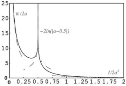
where the dimensionless quantity g, function of its dimen-sionless argument, is numerically evaluated and plotted as a continuous line in Fig. 3. The numerical evaluation is based on analytical expressions detailed in Appendix B, where the asymptotic behaviors of this function g are also derived, which are plotted in Fig. 3.

FIG. 2. Contour map of the elementary current perturbation due to a burnt fuse at the origin. The long-dashed curve corresponds to a 0 perturbation, the short-dashed one meets a saddle point at共␲,0兲, and corresponds to f共u,v兲=0.5.

IV. REGION OF MOST PROBABLE NEXT EVENT

We have now derived the number of cells associated with each current level, n共s兲, characterizing the interactions in this system, and need to consider some specific quenched disor-der to determine the typical separation between two subse-quent burning fuses. With a quenched disorder distribution of power-law type P共t兲=t␣ on 0艋t艋1, with ␣艌0, we obtain the cumulative distribution for thresholds to be below m, for the fuses that were still intact at current je, through Eq.共4兲,

as P共m,s兲 =m ␣_{共1 + s兲}␣_{− j} e ␣ 1 − je␣ He关m共1 + s兲 − je兴. 共12兲

We divide the space with respect to the last burned fuse in three zones, noted ⍀c, ⍀d, and ⍀f, and have to solve the

implicit Eq.共5兲 to find both the most probable region out of these three where the next break will happen, and the most probable value of the external current m at which the next fuse will burn. This equation becomes

冉

冕

⍀c +

冕

⍀d +

冕

⍀f

冊

n共s兲P共m,s兲ds = 1. 共13兲

By definition,⍀cis a region of fuses close to the last burned

one, with the largest positive current perturbation, such as

f共u,v兲⬎L/共2␲2ᐉ兲. All such fuses lie within a distance r

⬍

冑

共Lᐉ兲 of the last burned one, where we recall that ᐉ is the lattice step and L is the x dimension of the system.

⍀d is a region defined with moderate and finite current

perturbations, where L /共2␲2_{ᐉ兲⬎ f共u,v兲⬎}1

4. The typical

dis-tance r from the origin of the current perturbation, over the zone⍀d, is such as

冑

共Lᐉ兲⬍r⬍␲L.

Last,⍀f is a region of weak to negative current

perturba-tion, defined by the implicit equation f共u,v兲⬍1₄. It will be shown that when this region dominates the left-hand side of Eq. 共13兲, the leading contribution to it comes from points sitting at a characteristic distance r to the last burned fuse, scaling with the system size as r⬃Ly.

In Appendix C, we analyze in detail the three terms of Eq. 共13兲, and reformulate it as

Hc共␭兲 + Hd共␭兲 + Hf共␭兲 =

2␧共1 − je␣兲

je␣

, 共14兲 where␭=m/ je, with je, m the values of te external current at

the last break and at the most probable next one, ␧ =␲2_ᐉ2_/共2L2_{兲 and H}

c, Hd, Hfare proportional to the integrals

in Eq.共13兲 over the regions ⍀c,⍀d, and ⍀f.

We will classify the regime of the system according to the dominant term in the left-hand side of Eq.共14兲: If Hf

domi-nates, the system remains in a diffuse regime where there are no noticeable spatial correlations in the pattern of burnt fuse. If Hcdominates, this signifies the onset of a complete

local-ization regime where the damage will develop in a concen-trated zone scaling as the lattice size ᐉ, and propagate through the system, tearing it with jumps between successive events close to this smallest scale. Last, the dominance of Hd

would denote the onset of a diffuse localization regime, where the characteristic distance d between the burnt fuse scales as L, the system’s width.

Thus, following as the imposed current increases, which of the three terms dominates in Eq.共14兲, allows us to under-stand when damage starts to localize, and at which spatial scale. This allows us to classify, as function of the system dimensions Lx/ᐉ, Ly/ᐉ and of the quenched disorder,

char-acterized by␣, in which localization regime the system ends up in.

It is shown in Appendix C that in the early stages of the process, at small je, Hf dominates the solution of Eq.共14兲,

owing to the singularity of n共s兲 around s⬃0 共zero current perturbation line兲, and this equation reduces to

␭␣_{− 1 =} 1 − je␣

Ncellsje␣

. 共15兲

Since the first break is typically for j₁␣= 1 / Ncells, this

equa-tion predicts a second break typically at

␭1␣− 1 = 1, 共16兲

i.e., the second break should happen on average at j2=␭1j1

=共1+1兲1/␣j₁=共2/Ncells兲1/␣. Since j2⬎ j1, the process is stable

and there is a finite gap in the external current to trigger the next fuse burning. Since Hfis dominated by the asymptote of

zero current perturbation共noted h4 and h6 in Appendix C兲,

corresponding to the long dashed curve in Fig. 2, which spans the whole y range of the system, the next fuse is likely to burn at a distance scaling as d⬃Lyfrom the first one, i.e.,

the system remains in a diffuse regime, with no noticeable correlations between the locations of the burnt fuses: the size of the system wins compared to the attractive feature of the current concentration around the last burnt fuse, in a Flory-type argument. We can then proceed with this mean-field theory to treat the later stages of the process.

As long as Hfdominates Eq.共14兲, Eq. 共15兲 remains valid,

and by recurrence, we show in Appendix C that the nth fuse burns on average when the external current is such as

jn␣=共n/Ncells兲:. 共17兲

As long as this is the case, the nth weakest bonds are the most likely to be the n first burnt ones.

FIG. 3. Dimensionless number density of cells as function of the level of current perturbation, and asymptotic forms in dashed, at infinite distance共a=0兲, around the saddle point共a =1₂兲 and in the region close to the burnt fuse共a→⬁兲.

For threshold distributions characterized by a very large disorder, i.e., in the limit␣→0, it is shown in Appendix C that Hf共␭兲 always dominates in the solution of Eq. 共14兲, up to

the moment where je␣= 1

2. In this limit, the nth fuse burning

corresponds to the nth weakest threshold, and this lasts until the entire system is broken due to burned fuses percolating through the system. In this case, the process remains diffuse, in a percolationlike regime, up to the moment where P共je兲

=1₂, which corresponds to the critical percolation threshold. This means that in this limit of nonrenormalizability of the q.d. distribution, and very large disorder, the process is equivalent to a bond-percolation process, which was shown by Roux et al.关28兴.

On the contrary, for very small disorder, in the limit ␣

→ +⬁, we show in Appendix C that Hc共␭兲 dominates, and

even that the contribution of the nearest neighboring cells on the sides of the last burnt fuse dominate the integral: thus, the next fuses to burn are the ones carrying the highest cur-rent perturbation, and from the asymptotic expression of

Hc共␭兲 derived in Appendix C, and Eq. 共14兲, the level of next

break is set by ␭ = 21/␣ jes共␣兲1/␣ , 共18兲 where s共␣兲 =

冕

ᐉ/4␲L 1/4␲ _{共1 +␥兲}␣ 2␥2 d␥. 共19兲 This happens in a controlled way, i.e., for␭⬎1 if␣ is still sufficiently small so that s共␣兲⬍2N=2/ je␣, or through

imme-diate avalanches␭⬍1 in the opposite case. This is the limit of no disorder, where all bonds share the same threshold, and the concentration of current around the first broken one is the significant parameter controlling the process in this case: the rupture proceeds from the smallest scales, expanding through nearest neighbors from the initial seed to tear the system apart. This corresponds to a classical rupture process, analog to the rupture of a perfectly elastic and homogeneous mate-rial共no disorder兲, where the stress concentration at the tips of an initial default leads to the rupture of the system when the load is increased—in a stable way or not, depending on the load level—the situation known from one century in linear elastic fracture mechanics, treated by Griffith and Inglis关29兴. Between these two extreme cases, in the range of finite␣, the system can be driven to a third regime if Hddominates in

the solution of Eq.共14兲: correlations in the damage start to be significant, but the characteristic distance to the preceding burnt fuses is in a range between

冑

Lᐉ and L, and does not

scale as the lattice constant ᐉ: this is the regime which we refer to as “diffuse localization.”

We determine a lower value␣mof the exponent of the q.d.

distribution separating systems entirely equivalent to perco-lation up to breakdown, and these leading to diffuse localiza-tion, as follows: as long as the percolation regime holds, the value of the external current, and the size of the jumps␭ in it, are determined by Eq.共17兲. This regime goes on as long as Hd共␭兲 can indeed be neglected in front of Hf共␭兲. If both

terms become equal, the system transits towards the diffuse

localization regime, which is shown in Appendix C to corre-spond to leading order in 1 / Ncells, to the condition

␣ 2 ln

冉

L ᐉ

冊

= 2 1 − je␣ je␣ . 共20兲

If this condition is not met at the percolation threshold

je␣= 1 2, i.e. if ␣⬍␣m= 4 ln共L/ᐉ兲, 共21兲

the system always remains in the percolation universality class. If on contrary␣⬎␣m, the system undergoes a

transi-tion towards diffuse localizatransi-tion at a typical external current

jt= 1/关1 +␣ln共L/ᐉ兲/4兴1/␣. 共22兲

Similarly, we determine an upper cutoff␣M of the

expo-nent of the q.d. distribution, above which complete localiza-tion will prevail about the diffuse one. By equating Hf共␭兲

and Hc共␭兲, with ␭ evaluated from the percolation regime

expression in Eq. 共15兲, we show in Appendix C that this upper cutoff satisfies the implicit equation

s共␣M兲 − 2␲L/ᐉ

␣M

=ln共L/ᐉ兲

2 . 共23兲

From the expression of s, the equation above has a single solution at ␣M= 1. If ␣⬎1, the system will transit towards

complete localization at a characteristic current level

jt= 1/兵1 + 关s共␣兲 − 2␲L/ᐉ兴/2其1/␣. 共24兲

Eventually, if L /ᐉ⬍e4_{⯝54, the above would lead to}

␣M⬍␣m, and no diffuse localization is obtained for any

value of ␣. There is instead a transition directly from the percolation regime below␣⬍␣dto a regime leading to

com-plete localization for␣⬎␣d, with

s共␣d兲 − 2␲L ᐉ = ␲ ␧ ln

冉

1 am

冊

共␭perco␣ − 1兲 = 2. 共25兲

where␭percois estimated by Eq.共15兲. For␣⬎␣d, the system

starts a complete localization at a current level given by Eq. 共24兲.

To summarize the above results, a phase diagram of the system, showing the regime through which it will go to final breakdown, is shown in Fig. 4. The value of␣d was

deter-mined numerically from Eq.共25兲. A visual representation of sequences of burning fuses, for small systems, in five points of this phase diagram, illustrating the three regimes, is given in Fig. 1.

The above can be compared, in the limit of infinitely large systems, to the numerical analysis carried by Hansen et al. 关3兴: using the notations of this paper, ␣=␾0, and 1 /␾⬁= 0,

and the system goes from a disorderless regime A when␣ ⬎␣M= 1 to a scaling regime B with diffuse damage and

lo-calization when␣⬍␣M. The difference between the critical

exponent separating the two regimes, which is␣M= 1 in the

present case, and␾0= 2 in the models of 关3兴, is believed to

come from the elongated character of the systems considered here共LyⰇL兲.

Some remarks can be done on the succession of approxi-mations carried to establish this phase diagram: Most of these approximations correspond to keeping the leading or-der in the inverse of the number of lattice cells in the lateral dimension, ᐉ/L, for systems of infinite anisotropic ratio 共such as L/Ly→0兲. These approximations already take into

account finite size effects, since they keep finiteᐉ/L. They should thus be valid as long as these numbers areᐉⰆL, and

LⰆLy. Evaluating the following terms corresponding to

higher orders of the parameters ᐉ/L and L/Ly, in order to

estimate the quality of the asymptotic expansions reduced to leading order, is beyond the scope of the present work. In this analytical development, there is however an approxima-tion that does not fall in this category of asymptotic expan-sion: in order to evaluate whether the system departs from the percolationlike regime, as more and more fuses are burned and the system has stayed so far in this regime, we have considered separately the current perturbation triggered by each burned fuse. This is perfectly justified in the early stages of the process, where since the process is in a perco-lationlike regime, successively burned fuses are at distances of order Lyfrom each other, and almost do not interact.

How-ever, as the density of burned fuses increases, it can become finite共for sizes and q.d. where the process always remains in a percolation like regime, the density reaches eventually a large fraction, in principle, the percolation threshold兲. In this situation of a high fraction of burned fuses, the approxima-tion corresponding to evaluate the local current as a homo-geneous background je, superimposed to the perturbation

emanating from a single burned fuse 共the last burned one兲, becomes of lower quality, due to the existence of multiple close burned fuses anywhere in the system. Overcoming this limitation at high fractions of burned fuses, would require to take into account a large number of perturbation sources. This task seems more suitable for a purely numerical ap-proach: a main scope of this paper is to carry out the ana-lytical development in terms of extreme statistics for a mean-field theory going beyond the purely homogeneous description of damage 共i.e., incorporating a homogeneous term plus a local perturbation兲. Carrying out analytically the details of the calculation while keeping the track of every local perturbation is beyond the scope of this work. The

re-sult of this approximation is mainly to underestimate the number of close perturbation sources anywhere in the system as the process goes on: thus, this overestimates the weight of the probability to break far from the existing sources, Hf, and

underestimates the probability to enter a diffuse localization or a total localization regime. Thus, the mean-field theory presented here should predict properly the transition between “total” and “diffuse” localization regime, but should overes-timate the domain of the “percolationlike” regime: in Fig. 4, the left line should be located at smaller sizes. This approxi-mation seems to overestimate the transition size L /ᐉ by a finite factor not exceeding an order of magnitude, as will be shown in the next section.

Eventually, we note that in the diffuse localization regime, the process looks uncorrelated at the lattice constant scale, i.e., looks like a percolation system, but the arguments de-veloped in this paper show that damage starts to concentrate in a band of width scaling as the width of the system L. An argument based on percolation in a gradient corresponding to the structure of the damage concentration at the scale of the system can then be applied to describe the breakdown pro-cess, which sustains the arguments developed in关14兴 to ex-plain the origin of the roughness of the ultimate breakdown connected fronts in this regime.

Qualitatively, the phase diagram shown above supports the idea that the failure of natural macroscopic heteroge-neous systems is dominated by either the “total localization,” or the “diffuse localization” regime. Indeed, macroscopic materials are often systems much larger than the typical scale of the disorder, i.e., systems with a high ratio of system size over cell size, L / ell. In such regime, the present work pre-dicts that the percolation regime vanishes. More precisely, in this limit, the percolation regime would only subsist in the limit of nonnormalizable threshold distribution, correspond-ing to ␣→0. So the present work predicts that the break-down of such system is “totally localizing” at low disorder, or “diffusely localizating” at a larger one. This picture is consistent with the fracture properties of natural objects: when the fracturing solid is more homogeneous, or has only moderately disordered toughness properties, corresponding to large values of␣, the rupture is initiated on the weakest flaws, and the fracture propagates from nearest neighbor to nearest neighbor: this is the classical picture of linear elastic fracture mechanics of a homogeneous solid, described here as “total localization.” The fracture of such a regular object, as, e.g., a crystal, leaves a flat, or close to flat, fracture sur-face, as seen in Fig. 1共e兲. Conversely, when the toughness properties of the breaking solid are more scattered, i.e., at smaller␣, when the heterogeneous solid is more disordered, the rupture proceeds according to the “diffuse localization” regime 关illustrated in Fig. 1共b兲兴: this corresponds to the rough post mortem fracture surfaces observed in most natu-ral materials, found to be self-affine with a universal rough-ness of 0.8.

V. COMPARISON TO NUMERICAL SIMULATIONS

We now turn to confront this theory to numerical simula-tions of the fuse model. We consider rectangular models of

FIG. 4. Phase diagram of the system displaying the regime through which it will go to macroscopic breakdown, as a function of the system’s width and exponent characterizing the fuse thresh-old distribution.

L⫻Lycells, with high aspect ratios Ly/ L in order to be close

to the infinitely long cylinder considered so far. The lattice constantᐉ is now considered as unit length, the models con-sidered are periodic along the transverse x direction, and the rows of nodes at both lattice boundaries are set to two con-stant potential values, with a voltage drop⌬U between both regularly increased from 0. The rows of fuses are inclined at 45° with respect to the x and y directions. Current conserva-tion 共Kirchhoff equation兲 is required at each node, and the current through each fuse at location r connecting neighbor-ing nodes with a local potential drop ⌬V between them, is ⌬V if the fuse is intact, or 0 if the fuse is burned. This allows for each configuration of burned and intact fuses, to obtain by solving a linear system the voltage at each node, and the corresponding current map as j共r兲=C共r兲⌬U, where C共r兲 de-pends on the configuration of burned and intact fuses. The linear inversion is performed via a conjugate gradient algo-rithm 关Hestenes-Stiefel, Eqs. 共32兲–共38兲 in Ref. 关30兴兴. Ini-tially, the system is entirely intact and random thresholds of maximum sustainable current jt共r兲 are picked from the

quenched disorder distribution, independently for each fuse. At any stage of the process, the location r of the next fuse to burn and the corresponding value of the external current⌬U is obtained as⌬U=mins关jt共s兲/C共s兲兴= jt共r兲/C共r兲.

An example of configurations and the history of burning fuses is displayed in Fig. 1, for systems of size L⫻Ly= 30

⫻100, and values of␣between 0.25 and 2.5. The character-istic features of the three regimes are examplified in these cases.

For various values of L , Lyand of the exponent␣

charac-terizing the quenched disorder, we look at the distance d between two successive events, as function of its occurrence number in the succession of events up to total failure of the system共when a connected line separated the upper and lower boundaries of the system兲. This distance is averaged over 50 realizations.

The characteristic situation corresponding to ␣⬎1 is il-lustrated for the case of ␣= 1.5 in Fig. 5: the distance be-tween successive events is from a very early stage of order of a few unities, irrespectively, of the sizes L共4, 10, 20兲 and Ly

共200 and 2000兲 considered. This regime was referred above as total localization.

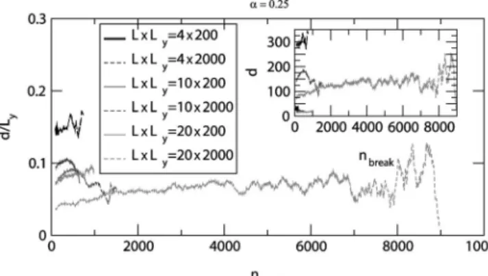
On the contrary, for low exponents ␣ corresponding to larger disorder, the typical situation is illustrated in Fig. 6 by the case of␣= 0.25: Simulations have been performed using lattice elongations Ly= 200 and Ly= 2000, and widths L = 4,

10 and 20. The distance between successive events has been averaged over 50 simulations. Even so, this quantity is still highly fluctuating, and an additional running average over 200 successive events is performed in order to extract the proper slow varying average of this distance. These high fluctuations are easily explainable: this regime is expected to be in the universality class of percolation, where the distri-bution of this distance at any stage is non-negligible for all possible distances in the lattice. Assuming consequently that the root of the variance of this distribution is of the same order as its average, the central limit theorem ensures that the root of the variance of the averaged distance over 50 realiza-tions is still of the order 1₇ of its average, which still corre-sponds to a high noise to signal ratio. The resulting average distance is plotted in Fig. 6, scaled by the lattice elongation

Ly in the main figure, or directly in lattice constant units in

the insert. This distance is found out to vary slightly during the process, and shows 50% variations between the different probed widths L, but the main result is that the average d is of order 0.1Ly, i.e. scales with Ly: this is consistent with the

prediction of the previous sections, that systems of infinite elongation Lyare isomorphic to percolation, i.e., that the

dis-tribution of burnt-out fuses is homogeneous, irrespectively of the configuration of the already burned fuses—which would predict for a very elongated system Ly→⬁, an average

dis-tance between successive events d⬃兰₀Ly兰

0 L_y

dy₁dy₂兩y₁

− y2兩/Ly2= Ly/ 3. The fact that we observe d⬃Ly/ 10 rather

than Ly/ 3 can be understood as a finite size effect: less cells

far away from the last fuse burning are likely to present the minimum ratio t / j, which increases the likelihood of having a next burned fuse in the zone of significant current pertur-bation, closer to the last burned fuse.

We have also analyzed the behavior of the system for␣ = 0.5, where according to Eq.共21兲, in the limit of Ly→⬁ one

FIG. 5. Total localization: distance between successive burning events, as a function of their index, averaged over 50 realizations. For a quenched disorder exponent␣=1.5, this distance remains of order unity, irrespectively of the dimensions L and Lyof the lattice.

FIG. 6. Fuse threshold distribution corresponding to exponent ␣=0.25: percolation universality class. Distance between succes-sive burning fuses, divided by the lattice elongation L_y, averaged over 50 realizations and 200 successive events. Irrespectively of the lattice dimensions, this distance is comparable to L_y共of order L_y/ 10 here兲. Note that this corresponds depending on the lattice dimen-sions, to an average distance d equal to 20–200 lattice units, as the inset shows, and equal to 1–10 times L.

expects a percolationlike behavior for L⬍e4/0.5_{⬃2980, or a}

diffuse localization behavior for larger system width. The average distance for L = 4, 10, 20 and Ly= 200 and 2000 is

displayed in Fig. 7—the inset represents the same data on a smaller scale. A qualitative interpretation of these results can be presented as follows: focusing first on the least elongated systems共Ly= 200兲, the average distance is for L=10 and 20

of a few units, but the thinest systems, L = 4, display a more complicated behavior: after an initial decrease, the distance displays episodes where its magnitude is around a few uni-ties, alternated with episodes of order Ly. This can be

inter-preted as a case on the verge between localizing or nonlocal-izing, i.e., as a case sitting around the line separating percolation from the localizing regime in Fig. 4. The value

L = 4 is considerably smaller than the predicted L⯝2980 for

infinitely elongated system. This presumably results from the underestimate in the analytical calculations, of the localizing and/or nonlocalizing separation due to the high fraction of burned fuse close to the breakdown process, and from strong finite-size effects at finite Ly, as explained in the previous

Section.

The presence of important finite size effects is confirmed by the fact that for more elongated systems, Ly= 2000, such

episodes where the average distance significantly exceeds the width of the system occur even more for the case L = 4, and appear also for the case L = 10, while they are absent from the case L = 20: presumably, the boundary between localizing and percolating systems is around L = 10 in that case. This means at finite elongations Ly, this boundary for any␣

cor-responds to significantly smaller L than value predicted for infinitely elongated systems. This finite size effect is ob-served to diminish for increasing elongations, as expected: the larger is the elongation Ly, the larger is the transition

width L. Due to numerical costs, it seems, however, difficult to evaluate numerically, in the limit Ly→⬁ where this finite

size effects would vanish, the exact transition value for the x-size separating non localizing systems and systems with diffuse localization, for example for such q.d. at ␣= 0.5. From the above, at finite Ly, this transition size at␣= 0.5 is

bounded between L = 10 共numerical observation for Ly

= 2000兲 and L⯝2980 关theoretical upper bound from the

mean field approach, Eq.共21兲兴. For practical numerical pur-poses at moderate system sizes, we note that such systems get into localizing regimes for x-system sizes L /ᐉ at one to two orders of magnitude than the previously derived upper bound, Eq.共21兲.

Eventually, in the localizing regimes, we need to distin-guish between what was referred to as diffuse or total local-ization in Sec. IV: total locallocal-ization was defined as a case where the most probable break after departing from percola-tion, would happen in the zone referred to as共1兲, i.e. corre-sponding to a distance r /ᐉ from the last burned fuse smaller than

冑

L /ᐉ. Diffuse localization corresponds to cases where

the next event would happen preferentially in zone 共2兲, at moderate current perturbations, which corresponds to dis-tances r /ᐉ from the last burned fuse ranging from

冑

L /ᐉ up to

a few L /ᐉ. A criterion to distinguish numerically between these two regimes is thus to look, for a fixed large elongation

Ly, whether the dependence of the average distance between

successive events over the system width is such as d /

冑

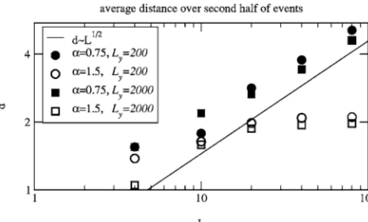
Lᐉ

vanishes at large L, or on the contrary remains finite or di-verges. In Fig. 8, the average distance between successive events was evaluated over 50 simulations and over the sec-ond half of the events before complete breakdown, which is in the localization regime for all cases probed. This average distance seems lowly sensitive to Ly= 200 or 2000共20%

dif-ference or less between both sizes兲, but the scaling as func-tion of L shows that this distance saturates rapidly for ␣ = 0.75, while it grows approximately as

冑

L for␣= 1.5. The extent over which this power law corresponds to slightly more than a decade for L, which is the maximum achievable numerically since the elongation Ly has to exceed

signifi-cantly L to be in the considered framework. This result is thus consistent with a transition from diffuse to total local-ization between␣= 0.75 and ␣= 1.5—the theory for Ly→⬁

predicts this transition at␣= 1. To pinpoint more accurately the precise value of the transition exponent 关between 0.75 and 1.5 is not easy numerically兴: this would require a priori to look at the scaling of d共L兲 over more orders of

magni-FIG. 7. ␣=0.5: features of localization, or of percolation, de-pending on L and Ly: Localization共short distance between

succes-sive events兲 is seen for larger L and smaller Ly, whereas episodes

with distances significantly larger than L are observed for short L and large Ly. Data averaged over 50 simulations.

FIG. 8. Distinction between total and diffuse localization: at elongations Ly= 200 or 2000, average distance d between

succes-sive events, for the second half of events, as function of the lateral size L of the system, on a bilogarithmic scale. Over the numerically accessible range as L grows, d is seen to saturate for␣=1.5, corre-sponding to total localization. For␣=0.75, d/L1/2_{does not vanish,}

tudes, for numerous ␣ inbetween, which would represent a significant numerical cost and was not the main objective of this work, performed mainly as a numerical check of the analytical derivations carried out in the previous sections.

VI. CONCLUSION

The main results of the analytical calculation presented in this paper are to be found in Fig. 4: There are three distinct phases of the fracture process depending on the disorder ex-ponent␣and on the ratio between the width of the lattice L and the lattice constant ᐉ when the lattice is a cylinder of infinite length. The first regime is a percolationlike regime where the distance between successive failing fuses is com-pletely random. In the second regime, named diffuse local-ization, the controlling parameter is L /ᐉ, while in the third regime, complete localization, the controlling length isᐉ.

To summarize the numerical results of Sec. V, regimes corresponding to percolation, diffuse and total localization have been clearly identified. The transition from diffuse to total localization is consistent with the predicted ␣= 1. The transition from percolation universality class to localizing regimes is seen to happen under increase of either the expo-nent␣ of the quenched disorder power-law distribution, or the width of the system, as predicted by the theory. Nonethe-less, the transition width for a given exponent was found significantly smaller for the systems of finite elongation stud-ied than for the infinite elongation system considered analyti-cally. This discrepancy was observed to be lower when the elongation Lyincreased, and presumably corresponds to

im-portant finite size effects. The transition from diffuse to total localization is consistent with the predicted ␣= 1, irrespec-tively of the system’s elongation.

Hence, in the diffuse localization phase, we expect a smooth variation of the damage profile scales L, while there is still no strong localization driving the burned fuse to merge at the lattice constant scale: the region where argu-ments based on the percolation in gradient should apply. In this case, the shape of the dipolar current perturbation共Fig. 2兲, leads to most probable relative positions 共x,y兲 of the next burned fuse relative to the last one, for which x and y are of the same order of magnitude, which is at the origin of the smooth quadratic maximum of the damage profile as func-tion of y, as observed in关14兴: This confirms the scaling ar-guments used to relate to roughness exponents and correla-tion length divergence exponents in such systems.

APPENDIX A: STATISTICAL LEMMAS

Consider p different types of random variables y, charac-terized by their cumulative distributions Pi共y兲 and

probabil-ity density functions pi共y兲=dPi共y兲/dy= Pi

⬘

共y兲, for i

= 1 , . . . , p. Next, consider an ensemble of n1 random

vari-ables distributed according to p1, n2 according to p2, . . . , np

according to np. In the limit where N =兺i=1 p

niⰇ1, we wish to

characterize

m =具min_{兵i=1,. . .,p,j=1,. . .,n}

i其yi,j典. 共A1兲

The probability that some particular variable number j of type i, yi,j, would be equal to x, while all others are larger, is

pi共x兲关1 − Pi共x兲兴ni−1

兿

j_⫽i

关1 − Pj共x兲兴nj. 共A2兲

The probability that any of the variables of type i would be the smallest and equal to x, is the above times a factor ni.

Thus, the wanted quantity may be written as

m =

冕

x dx

兺

i=1 p

冋

nipi共x兲关1 − Pi共x兲兴ni−1

兿

j⫽i 关1 − Pj共x兲兴nj

册

=

冕

x dxd dx

冋

兿

_j=1 p 关1 − Pj共x兲兴nj

册

=

冕

dx

冋

兿

j=1 p 关1 − Pj共x兲兴nj

册

. 共A3兲

Setting p = 1 in Eq.共A3兲, we have that

m =

冕

dx关1 − P1共x兲兴N. 共A4兲

Since the function 1 − P1共x兲 decreases continuously from 1 to

0, for large n the product 关1− P1共x兲兴N is equal to 1 for x

⬍xc, up to a certain cutoff xc, above which it becomes

van-ishingly small. The integral Eq.共A4兲 is then simply equal to

xc. We determine xc by invoking the standard saddle point

approximation, which leads to the equation

p₁

⬘

共xc兲

p1共xc兲

=共N − 1兲 p1共xc兲 1 − P1共xc兲

共A5兲 for xc. By using l’Hôpital’s rule, p1

⬘

/ p1⬇p1/ P1, this equation

reduces to the condition NP共xc兲=1. Using m=xc, we have

关25兴

NP1共m兲 = 1. 共A6兲

Generalizing this result to p⬎1, we find by invoking the saddle point approximation for Eq.共A3兲, the equation

兺

i=1 p

冉

nipi共m兲 1 − Pi共m兲

冊

⬘

=

冉

兺

j=1 p njpj共m兲 1 − Pj共m兲

冊

2 . 共A7兲 If we now set 1 − Pj共m兲⬇1 as Pj共m兲Ⰶ1, and use l’Hôpital’s

rule,

兺

i=1 p nipi

⬘

共m兲

兺

j=1 p njpj共m兲 ⬇

兺

i=1 p nipi共m兲

兺

j=1 p njPj共m兲 , 共A8兲

Eq.共A7兲 reduces to

兺

j=1 p

njPj共m兲 = 1, 共A9兲

which generalizes Eq.共A6兲.

In the case of an infinite number of random variables indexed by a continuous parameter s, the equivalent of Eq. 共A9兲 is

冕

s

n共s兲P共m,s兲ds = 1. 共A10兲

The probability Qi that the minimum variable would be of

type i 共for a discrete set of random variables兲, is from the above

Qi=

冕

dx

冋

nipi共x兲关1 − Pi共x兲兴ni−1

兿

j⫽i

关1 − Pj共x兲兴nj

册

.

共A11兲 The same argument shows that 关1− Pi共x兲兴ni−1兿j⫽i关1

− Pj共x兲兴nj is equivalent to 1 when x⬍m, or 0 when x⬎m.

Thus,

Qi=

冕

x=−⬁

m

dx nipi共x兲 = niPi共m兲. 共A12兲

For a continuous set of random variables, the probability that the minimum variable would correspond to an index s 苸关s1, s2兴 is then Q_关s 1,s2兴=

冕

s₁ s₂ n共s兲P共m,s兲ds. 共A13兲

APPENDIX B: DENSITY OF CELLS PER LEVEL OF SUSTAINED CURRENT

To compute n共s兲, we will use an explicit expression va共u兲

of the contours of isoperturbation, shown in Fig. 2 defined implicitly as

f„u,va共u兲… = a. 共B1兲

Inverting this expression from Eqs.共10兲 and 共B1兲, comes the following: if a⬍0, there are two points of abcissa u satisfy-ing this. Their ordinates are

va±共u兲 = a cosh

冋

2a − 1 2a cos共u兲 ±

冑

cos2共u兲 4a2 + sin2共u兲 a

册

. 共B2兲 These functions are defined for

u mod关2␲兴 苸 关− ua max ,ua max_兴, with ua max

= a cos关4a/共4a−1兲兴. If 0⬍a⬍0.5, there is a single defined functionva共u兲 satisfying Eq. 共B1兲 for any u, which is

the positive alternative of the above Eq. 共B2兲. Last, if a ⬎0.5, the expression of va共u兲 is identical, but once again this

function has a finite support u mod关2␲兴苸关−ua max

, ua

max_{兴, with}

u_amax= a cos共1−1/a兲. Some examples of these auxiliary quan-tities were set in Fig. 2.

To compute n共s兲, we reformulate the condition j苸关je共1+s兲, je共1+s+⌬s兲兴 as f共u,v兲苸关a,a+⌬a兴 where a

= 2L2s /共␲2ᐉ2兲 and ⌬a=2L2⌬s/共␲2ᐉ2兲 from Eq. 共9兲, which

through a Taylor expansion of f共u,v兲 in v around va共u兲

de-fines

⍀共s,⌬s兲 = 兵共u,v兲/v 苸 关va共u兲 − wa共u兲⌬a,va共u兲兴其, 共B3兲

wa共u兲 = − 1/

⳵f

⳵v关u,va共u兲兴, 共B4兲

and thus n共s兲= 1

⌬sᐉ2兰共x,y兲苸⍀共s,⌬s兲dx dy can be expressed as

n共s兲 = 2L 4 ␲2_ᐉ4g共2L 2_s/␲2_ᐉ2_{兲, 共B5兲} where g共a兲 =

冕

u=0 min共ua max_,␲兲 wa共u兲du. 共B6兲

This number density g共a兲 was numerically evaluated from the above and displayed in Fig. 3. We will also derive below the asymptotic behavior of this function around the special values a⬃0, infinitely away from the burnt fuse, a→ +⬁, around for the near neighbors of the broken fuse, and a ⬃0.5, around the saddle point 共u=␲, v = 0兲. As will be

shown straightforwardly, these asymptots, displayed in Fig. 3, are

g共a兲⬃a→0␲/2兩a兩, 共B7兲

g共␦a + 1/2兲⬃_␦a→0− 2 ln共兩␦a兩兲, 共B8兲

g共a兲⬃a_→±⬁1/2a2. 共B9兲

Indeed, from Eq.共10兲,

wa共u兲 = − 1/

⳵f

⳵v关u,va共u兲兴

= 关cosh„va共u兲… − cos„u…兴

3

sinh„va共u兲…关cos2共u兲 + cos共u兲cosh„va共u兲… − 2兴

, 共B10兲 whereva共u兲 is given by Eq. 共B2兲.

Developing the above around a⬃0+_{to main order in a is}

a direct exercise which leads to wa共u兲⬃−1/a when u

苸关␲/ 2 ,␲兴, and 兩wa共u兲兩Ⰶ1/a for u苸关0,␲/ 2兴. The

integra-tion of wa共u兲 in Eq. 共B6兲 leads then to the asymptotic value

in Eq.共B7兲.

Conversely, around a⬃ +⬁, f共u,v兲⬃2共u2_−v2_兲/共u2_+v2_兲2

= 2 cos共2␪兲/r2_{, where u / r = cos␪ and v / r = sin␪. Then,}

defining, I共a兲 =

冕

u⬎0,v⬎0,f共u,v兲⬍a du dv, we have g共a兲 = − dI共a兲/da, 共B11兲

and in polar coordinates

I共a兲 =

冕

␪=0 ␲/4

冕

r=0 冑2 cos共2␪兲/a r dr d␪= 1/2a, 共B12兲

leading to the asymptotic form g共a兲⬃1/2a2_{, Eq.共B9兲.}

Eventually, around␦a = a −1₂⬃0, we reformulate the

second order in v: ␦f = f共u,v兲−1/2= f共u,v兲− f关u,v0.5共u兲兴

⬃⳵vf关u,v0.5共u兲兴␦v +⳵vvf关u,v0.5共u兲兴␦v2/ 2. The first term

dominates if ␦a⬍兩2共⳵_vf兲2_/⳵

vvf兩 and then 0⬍␦f⬍␦a is

equivalent to 0⬍␦v⬍−␦a /⳵_vf. When␦a⬎2共␦_vf兲2_/⳵ vvf, we

will have兩␦f兩⬍␦a if 0⬍␦v⬍

冑

␦a /⳵vvf. From Eqs.共B2兲 and

共B10兲, v0.5共u兲=

冑

2 − cos2共u兲, and ⳵vf关u,v0.5共u兲兴 has a single

zero in u =␲ 共saddle point兲, ⳵vf⬃共␲− u兲/4, whereas

⳵vvf关u,v0.5共u兲兴 remains finite, tending towards a finite value

␣when u→␲. Thus, we have

冕

u,v/f共u,v兲苸关0.5−␦a,0.5兴 du dv, 共B13兲 ⯝␦a

冕

0 ␲−冑␦a/8␣_{− 4du} ␲− u + O共␦a兲, ⯝− 2␦a ln共␦a兲 + O共␦a兲. 共B14兲

Differentiating this expression with respect to␦a shows that g共0.5−␦a兲⬃−2 ln共␦a兲, for␦a→0+_{. Similar arguments lead}

to the same asymptotic form for a negative␦a, i.e., to the

asymptotic form in Eq.共B8兲.

APPENDIX C: SPATIAL DIVISION OF THE INTEGRAL CHARACTERIZING EXTREME STATISTICS

Here, we present the details of the subterms intervening in the implicit Eq.共5兲, which determine both the region of the most probable next break with respect to the previous one, and the most probable jump in external current to reach this next break.

We have to solve the implicit Eq. 共5兲, with a derived distribution P共m,s兲 =m ␣_{共1 + s兲}␣_{− j} e ␣ 1 − je␣ He„m共1 + s兲 − je…. 共C1兲

coming from the assumed quenched disorder distribution,

P共t兲=t␣ on 0艋t艋1, with ␣艌0, transformed into a condi-tional probability of breaking for fuses having so far sur-vived, using Eq.共4兲.

In the integrand of Eq.共5兲, n共s兲 is expressed as function of g共a兲 through Eq. 共11兲, and we approximate this last func-tion by its asymptotic forms Eqs.共B7兲–共B9兲 around the sin-gularities and in the tail of highest perturbations. We divide the support of the integral in seven zones.

共1兲 In the neighboring cells carrying maximum current, such as r /ᐉ⬍c where c is a finite large number. The nearest neighbors on the sides of the last broken cell carry the maxi-mum current, ␦j / je= f共2␲ᐉ/L,0兲␲2ᐉ2/ 2L2=

1

4,

correspond-ing to an upper cutoff aM= L2/ 2␲2ᐉ2. Close to the origin, the

current perturbation falls as 1 / r2_{, and this close zone is then}

defined by the condition aM/ c2⬍ f共u,v兲⬍aM.

共2兲 The cells carrying a current such as 3

4⬍ f共u,v兲

⬍c2_{/ 2␲}2_{. On the x axis, from Eq. 共10兲, these conditions}

correspond to 2L / c⬍x⬍a cos

共

−1₃

兲

L / 2␲⯝L/3. We require

that these two defined first zones have a common boundary, which by equating the cutoffs of f sets c2= L /ᐉ.

共3兲 A zone around the saddle point, defined as 1 4

⬍ f共u,v兲⬍3 4.

共4兲 A zone such as am⬍ f共u,v兲⬍1/4. This zone includes

the far-range from the last broken fuse, on which the current is slightly increased by its presence. The lower cutoff amis

determined by the y extent of the system 共length of the band兲, which was so far omitted. When the finite aspect of Ly

is taken into account, the current perturbation derived from boundary conditions at infinity, Eqs.共9兲 and 共10兲 is still valid in boundary conditions corresponding to setting the global current through the top and bottom plate, i.e.,

冕

x=−L/2 L/2

yˆj共x, ± Ly/2兲dx/L = jo.

Indeed, we find for LyⰇL, that

f共u,␲Ly/L兲 ⯝ − cos共u兲/cosh共␲Ly/L兲

⯝ − cos共u兲exp共−␲Ly/L兲,

whose integral is zero for u苸关−␲,␲兴. However, when counting the number of cells sustaining a given current, the condition兩y兩⬍Ly/ 2 should be added to derive n共s兲. From the

above, n共s兲 is unmodified when a⬎am= exp共−␲Ly/ L兲, or

when a⬍−am, but in the neighborhood of zero for −am⬍a

⬍am, n共s兲 has to be modified according to

g共a兲 =1

a关a cos共− a/am兲 −␲/2兴. 共C2兲

This function is pair, and increasing for a艌0 from g共0兲 = 1 / amto g共am兲=␲/ 2am.

共5兲 A tiny zone of vanishing current perturbation, −am

⬍ f共u,v兲⬍am, for which n共s兲 has just been determined.

共6兲 A far-range zone where the current is screened by the last burnt fuse, −1⬍ f共u,v兲⬍−am.

共7兲 A zone of a highly screened current, −aM⬍ f共u,v兲⬍

−1.

The zones corresponding to regions defined as ⍀c, ⍀d,

and ⍀f in Sec. IV, are, respectively, regions 共1兲–共7兲. They

correspond to regions, which are with respect to the last break, either close to it, at distances comparable with the lattice step, or diffusively close, at distances comparable to the width of the system Ly, or “far,” at distances comparable

with the system size LyⰇLx. Dividing here in seven

subre-gions, will allow us to use asymptotic forms of the seven corresponding subintegrals.

We will classify the regime of the system according to the zone where most of the integral in Eq. 共5兲 is realized: We expect this zone to be either共4兲–共6兲, in which case the sys-tem remains in a diffuse regime where there are no notice-able spatial correlations in the pattern of burnt fuse, or 共1兲, which signifys the onset of a complete localization regime where the damage will develop in a concentrated zone scal-ing as the lattice sizeᐉ, and tear through the system starting from this smallest scale, or共2兲 and 共3兲, which would denote the onset of a diffuse localization regime, where the charac-teristic distance d between the burnt fuse scales as L, the system’s width.