Dynamic Performance of Nonlinear 100X
Displacement Amplification Piezoelectric Actuator
The MIT Faculty has made this article openly available.
Please share
how this access benefits you. Your story matters.
Citation
Neal, Devin, and H. Harry Asada. “Dynamic Performance of
Nonlinear 100X Displacement Amplification Piezoelectric Actuator.”
ASME 2010 Dynamic Systems and Control Conference, Volume 2,
12-15 September, 2010, Cambridge, Massachusetts, ASME, 2010,
pp. 65–72. © 2010 by ASME
As Published
http://dx.doi.org/10.1115/DSCC2010-4227
Publisher
ASME International
Version
Final published version
Citable link
http://hdl.handle.net/1721.1/118785
Terms of Use
Article is made available in accordance with the publisher's
policy and may be subject to US copyright law. Please refer to the
publisher's site for terms of use.
DYNAMIC PERFORMANCE OF NONLINEAR 100X DISPLACEMENT AMPLIFICATION
PIEZOELECTRIC ACTUATOR
Devin Neal H.Harry Asada Mechanical Engineering MIT Cambridge, MA 02139 [email protected] ABSTRACTThe dynamic frequency response of a nonlinear piezoelectric amplification mechanism capable of over 150 fold displacement amplification is presented. Research to amplify the displacement of piezoelectric actuators has included flexure based approaches that utilize geometric configuration, and has included frequency based approaches that utilize resonance and small steps to contribute to a full motion. The dynamic operation of the actuator presented here utilizes the benefits from both of these methods. The geometry allows for great displacement amplification, and operation within a specific frequency band allows for the exploitation of a nonlinear singularity. The actuator has three distinct modes of dynamic operation, one of which achieves significant displacement by utilizing momentum to pass through a singular configuration. A nonlinear model, linear models for each frequency response mode, and multiple prototypes are presented. This actuator operating in the high displacement frequency band is promising as an input actuator for stepping mechanisms.
INTRODUCTION
Piezoelectric actuators have a number of salient features, including high stress, high bandwidth, and high power density along with stable and reliable material properties. Despite valuable features, the greatest shortcoming of piezoelectric actuators is the limited strain they produce. Strains of PZT stacks are on the order of 0.1%, well below skeletal muscles and other smart actuator materials. Displacement amplification has been a subject of piezoelectric actuator research for the past several decades. A number of methods have been developed, which can be classified into internally leveraged (bi-morph bending cantilevers, and uni-morph bowing actuators), externally leveraged (lever arm, hydraulic, and flextensional actuators), and
frequency leveraged actuators (inchworm, and ultrasonic actuators) [1]. Internally leveraged actuators exhibit substantial displacement but with significantly decreased force due to the strain energy absorbed in bending and low stiffness. Frequency leveraged actuators rely on friction of contacting surfaces, which varies depending on pressure and surface conditions. Applications are limited to light duty, and open-loop repeatability is limited [2]. This paper focuses on a novel type of flextensional displacement amplification. Flexure based amplification methods have been studied extensively. They were originally designed for acoustic purposes, but have since been designed to maximize output displacement and force [3]. These actuators include the Moonie [4] and the Cymbal [5]. These designs are modular and have been stacked serially to increase net displacement [6]. Most of the flextensional mechanisms use a rhombus-type amplification structure. A single rhombus can produce approximately 10 times larger displacement. In an attempt to gain a larger effective strain, nested amplification mechanisms have been developed. Using two layers of the rhombus-type amplification, over 20% effective strain has been obtained, where the effective strain is defined to be the ratio of output displacement to actuator body length along the axis of output displacement [7].
This paper presents an alternative method, which can produce over 100 times larger displacement in a single stage. The key idea is to exploit “buckling”, a pronounced nonlinearity of structural mechanics. While this nonlinear and singular phenomenon can produce an order-of-magnitude larger displacement amplification than typical flexure based methods, buckling is an unstable, unpredictable phenomenon. Nonlinear stiffness characteristics are not inherently negative though. For example, the unstable stiffness characteristics of a similar bi-stable element have been utilized to shape the force-displacement profile of dialectric
Proceedings of the ASME 2010 Dynamic Systems and Control Conference DSCC2010 September 12-15, 2010, Cambridge, Massachusetts, USA
polymer actuators [8]. Additionally, the unpredictability of buckling can be controlled. In our previous publications, methods for controlling the direction of buckling were developed by using an additional mechanical stiffness, and by asynchronously activating multiple phase arrayed buckling actuators [9], [10].
This paper extends the buckling concept to dynamic operation. It bridges a gap between frequency leveraged actuators and externally leveraged actuators. Passing through the singularity and providing power to a load on both sides can be effectively accomplished within a specific freque
ncy band by utilizing the momentum of the load.
The buckling actuator principle is discussed, followed by the derivation of the nonlinear dynamic equation. Next linearized models are provided for the 3 modes of operation that can occur. Results are verified experimentally and discussed.
PRINCIPLE AND METHODS OF BUCKLING CONTROL [9]
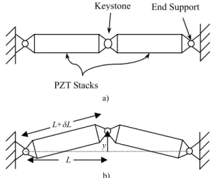
Figure 1 shows the schematic of a nonlinear, large-strain buckling piezoelectric actuator, consisting of a pair of piezoelectric stacks and a monolithic structure. The monolithic structure mechanically grounds the piezoelectric stacks between a “keystone” output node and the end supports placed at both sides. The end supports, and output node are connected to the piezoelectric stacks through rotational joints.
As the PZT stacks are activated, they tend to elongate, generating a large stress along the longitudinal direction. When the two PZT stacks are aligned, the longitudinal forces cancel out, creating an unstable equilibrium. With disturbance, the PZT stacks tend to “buckle” as illustrated in Fig. 1(b). Let δL be the unforced elongation of each PZT stack and y be the vertical displacement of the keystone output node. Differentiating the kinematic relation, y2=(L+δL)2-L2, in terms of δL and ignoring
higher-order small quantities yields the following amplification ratio, G, , as 0 L G y y . (1)
This is a type of kinematic singularity at y = 0. Even for a finite piezoelectric displacement, the amplification gain, G, is significantly large. Although this buckling mechanism can provide extremely large displacement amplification, buckling is in general an unpredictable, erratic phenomenon. It is not feasible to quasi-statically bring the output keystone from one side to the other across the middle point. Once it goes upwards, it tends to stay there, and vice versa. This is in a sense “mono-polar” activation where the stroke of the output keystone is about half of the total possible displacement. Therefore, it is desirable to have the capability to pass through the singularity point to the other side once buckling has occurred to achieve “bipolar” activation. To achieve this “bipolar” activation, previous methods have utilized additional mechanical stiffness elements [9] and utilized multiple buckling actuators to guide each other through their respective singularity points [10]. This paper presents an alternative approach: dynamically activating a single buckling actuator and utilizing the momentum of the load to pass the output through the singularity point at y=0. This relies on the nonlinear stiffness characteristics of the actuator which are analyzed next.
FIGURE. 1. BUCKLING ACTUATOR CONSISTEND OF 2 PIEZOELECTRIC STACK ACTUATORS ARANGED FACE TO
FACE
NONLINEAR DYNAMIC MODEL
The buckling actuator can be modeled as a series of two springs in parallel between two grounded nodes as shown in Fig. 2. For the ideal actuators, the length of each spring at the singularity point shown in Fig. 2 a) would be equal to the rest length of each spring. However this is not physically realizable due to manufacturing tolerances, nor necessarily desirable due to preload benefits. A preload is achieved by positioning the grounded ends of the buckling actuator a preload displacement length, lp, closer to the center than the rest length of the spring, L.
Preload is beneficial because it eliminates nonlinear, and generally overly compliant initial contact stress. It is preferred to not adhesively connect the PZT stacks to the grounded nodes for two reasons. First, adhesive or other coupling methods would introduce additional compliance in series with the PZT stacks, and second, the coupling should not be used in tension because the PZT stacks of ceramic layers could become delaminated due to cyclic tensile stresses. Compliance from any source that is in series with the PZT stacks degrades output performance by storing strain energy that could be otherwise applied to the load upon activation. With sufficient preload, the PZT stacks stay in contact and don’t slip on the node contact surfaces.
The activation of the PZT stacks are modeled as effectively changing the rest length of the springs from L to L + δL. With this model, the potential energy, U, stored in a spring can be calculated as a function of δL and output displacement, y. The length of the spring can be seen geometrically in Fig. 2 b) and the rest length is modified by the PZT stack input, δL.
PZT Stacks
Keystone End Support
L+δL y L
a)
FIGURE 2. MODEL OF BUCKLING ACTUATOR AS SERIES OF 2 SPRINGS OF RESLT LENGTH L + ∆L
2
2 21
2
pU
k
y
L l
L
L
(2)The negative derivative of U with respect to y yields the force along the output axis exerted by the buckling actuator.
2(
)
2 pL
L ky
dU
F
ky
dy
y
L l
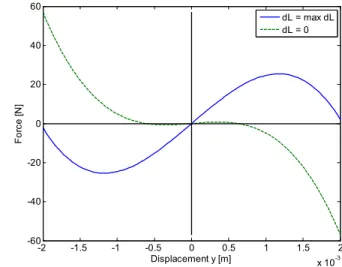
(3)A plot of the force vs. output displacement is shown in Fig. 3. Notice the large region near y = 0 that has positive slope. Positive slope indicates instability, further showing that the singularity point at y = 0 is unstable. The parameter values for this plot are based on realized prototypes using 40 mm PZT stack actuators with a maximum free displacement of 42µm [11]. The stiffness, k, is calculated based on the geometry and material properties of the flexures, as well as the stiffness of the PZT stacks as described in [12]. The bending stiffness of the flexures was calculated and accounted for but proved to be insignificant and was neglected. The preload displacement, lp, is on the same order as dL; ranging
from 0 to 42 micrometers.
The force from this actuator is exerted on a load modeled as a mass of mass m, and damper of damping coefficient b. The full dynamic equation of interest is then,
2(
)
2 pL
L ky
my by ky
y
L l
(4)The mass is approximated as constant despite the fact that the PZT stacks are rotating and their effective mass is changing. This is because, the angular displacement is very small, and total mass contributed by the stacks is also small. The damping is also assumed to be constant because small changes in damping have little effect on the frequency based analysis for which simulation is used. Simulation of this nonlinear model, and experimental evaluation demonstrate that there are 3 distinct frequency response modes. These modes are discussed in the next section.
LINEARIZED MODELS OF DYNAMIC SYSTEM
Three modes of oscillations have been observed in this actuator. The first is an approximately linear mode in which mono-polar displacement is observed for lower frequencies and the magnitude of the oscillations are largely independent of frequency. The second mode is bipolar oscillation and is observed in a single band of frequencies. This second mode is the most interesting because it results in the most power transferred from the actuator to the load and exists at a frequency band that is tunable to specific applications. The third and final mode is again mono-polar displacement, is highly linear due to small displacements, and the magnitude decreases sharply with increased activation frequency.
-2 -1.5 -1 -0.5 0 0.5 1 1.5 2 x 10⁻³ -60 -40 -20 0 20 40 60 Displacement y [m] Fo rc e [N ] dL = max dL dL = 0
FIGURE 3. FORCE VS. DISPLACEMENT FOR A BUCKLING ACTUATOR WITH MAXIMUM PIEZOELECTRIC ACTIVATION
(DL = MAX DL), AND ZERO ACTIVATION (DL = 0)
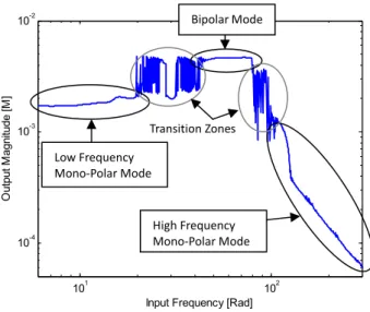
To see each mode clearly, the nonlinear model was simulated by driving δL between 0 and 42 µm over a range of frequencies. Many oscillation cycles were simulated to allow any transient effects to attenuate. The magnitude of the last complete output oscillation was then recorded as the magnitude of the response. The results are plotted in Fig. 4. This is similar to the magnitude plot of a bode diagram. The phase plot of a bode diagram is not presented because it does not make physical sense to plot for this system because the output frequency is not equal to the input frequency during bipolar activation. In fact, for bipolar activation, the output frequency is exactly ½ of the input frequency. The first flat region in Fig. 4 is the first mono-polar frequency response mode. Next, there is a transition band of frequencies at which the output passes though the singularity position but there is no steady state solution. Then there is the bipolar mode. In this frequency band, the output passes through the singularity point with each oscillation of the input PZT actuators and there exist steady state solutions. Next, there is another transition band, followed by the high frequency mono-polar mode. L k O k O y a) b) lp L-lp
We now present linearized models of these modes in order to gain a better understanding and intuition of the dynamic system.
101 102
10-4 10-3
10-2
Input Frequency [Rad]
O ut put M agnit ude [ M ]
FIGURE 4. OUTPUT DISPLACEMENT MAGNITUDE RESPONSE AS A FUNCTION OF FREQUENCY OF DRIVING
PZT STACKS SIMULATED USING NONLINEAR MODEL
Low Frequency Mono-Polar Mode
The first mode is in a relatively linear region of displacement. A diagram of this mode of oscillation is shown in Fig. 5 a). As the input PZT actuators activate, the total displacement does not change dramatically. Therefore selecting the displacement at the mean level of activation as the operating point lends itself well to linearization via Taylor expansion. The linearized force from Eq. (3) is,
0 0 2 2 0 2 0 0 0 0 3/ 2 2 2 2 2 0 0 , ( ) 1 ( ) ( ) p p p ky F L y L L y L l L L y L L k y y y L l y L l
, (5)where δL0 is the mean value of δL (δLmax/2), and y0 is the value of
y where the force from the actuator is zero,
2 2
0
(
0)
(
p)
y
L
L
L l
.
The results of the linearization of the force function are shown in Fig. 6. We see that the linearized model does a good job of capturing the frequency and magnitude properties of the nonlinear model.
The nonlinear model shows slightly less displacement than the linearized model because of the nonlinearities. At greater displacement, the stiffness increases and pulls the output node down, while at lower displacement, the stiffness is lower and allows the displacement to reach further down. If the magnitude
of the input displacement, δL, is greatly reduced, then the nonlinear effects are greatly reduced as well. In such a case, the nonlinear and linear models align almost exactly.
FIGURE 5. (A) FIRST AND THIRD OSCILLATION MODES: LOW AND HIGH FREQUENCY MONO-POLAR DISPLACEMENT. (B) SECOND MODE: MID FREQUENCY
BIPOLAR DISPLACEMENT 0 0.5 1 1.5 2 2.5 3 3.5 4 0.4 0.6 0.8 1 1.2 1.4 1.6 1.8 2 2.2x 10 -3 Time [s] Di spl a ce m ent y [ m ] Nonlinear Model Linearized Model
FIGURE 6. SIMULATION OF NONLINEAR AND LINEAR MODEL AT LOW FREQUENCY (1 HZ)
High Frequency Mono-Polar Mode
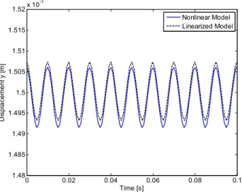
Additionally, at frequencies higher than the range in which bipolar oscillation occurs, the linearized model matches very well with the linear model derived via first order Taylor expansion. This is due to the nonlinear model having low magnitude oscillations at high frequencies and behaving very linear at such high frequencies. A diagram of this oscillation mode is shown in Fig. 5 a). An example of the output performance of both the linear and nonlinear models simulated at high frequency is plotted in Fig. 7. Notice that the magnitude in the high frequency simulation (Fig. 7) has dropped significantly from the low frequency simulation (Fig. 6).
O y0 O a) b) Low Frequency Mono‐Polar Mode Bipolar Mode High Frequency Mono‐Polar Mode Transition Zones
Mid Frequency Bipolar Mode
The linear model begins to break down as the frequency approaches the range at which bipolar activation occurs. This is shown in Fig. 8. As the frequency approaches the damped natural frequency of the linearized model, the magnitude of the oscillations increase for both the nonlinear and linear models. When the magnitude is sufficiently high, the linear model will have reached a displacement close to the singularity at y = 0, and the nonlinear model will reach a negative displacement value. When this happens, the nonlinear model will pass through the singularity point to the other side. However, the nonlinear model will not necessarily continue to pass through the singularity with each input cycle. This is demonstrated in Fig. 8 where the nonlinear model passes through the singularity at about 0.3 s, settles in the linear regime on the other side from 0.3-0.7 s, builds in magnitude in the linear regime, and then passes through again at 0.7 s once the oscillation magnitude is sufficiently high again.
0 0.02 0.04 0.06 0.08 0.1 1.48 1.485 1.49 1.495 1.5 1.505 1.51 1.515 1.52x 10 -3 Time [s] Di spl a ce m ent y [ m ] Nonlinear Model Linearized Model
FIGURE 7. SIMULATION OF NONLINEAR AND LINEAR MODEL AT HIGH FREQUENCY (100 HZ)
0 0.5 1 1.5 2 -3 -2 -1 0 1 2 3x 10 -3 Time [s] D is p la cem ent y [ m ] Nonlinear Model Linearized Model
FIGURE 8. SIMULATION OF NONLINEAR AND LINEARIZED MODELS DEMONSTRATING A TRANSITION FREQUENCY (7 HZ) BETWEEN LOW FREQUENCY MONOPOLAR MODE AND
BIPOLAR MODE
The linear model of Eq. (5) is ineffective at providing any valuable information at frequencies in the range of bipolar oscillations. The models simulated in this frequency band are shown in Fig. 9. At this frequency, the magnitude of the nonlinear model is much greater than the linear model, and centered about a displacement of 0 rather than the operating point at which the linear model was linearized about. A diagram of this bipolar mode of operation is shown if Fig 4 b).
To formulate a linearized model of the bipolar frequency response of the nonlinear model, Taylor series expansion is insufficient. This is because the mean value of displacement to linearize about is zero, i.e. y0 = 0, and the first order term does not
capture the dependence of stiffness on the magnitude of the oscillation. 0 0.2 0.4 0.6 0.8 1 1.2 1.4 -3 -2 -1 0 1 2 3 4x 10 -3 Time [s] Di spl a ce m ent y [ m ] Nonlinear Model Linearized Model
FIGURE 9. SIMULATION OF NONLINEAR MODEL AND LINEARIZED MODEL ACTIVATED AT A FREQUENCY (10 HZ)
HIGHER THAN THE DAMPED NATURAL FREUQUENCY OF THE LINEARIZED MODEL (9.6 HZ)
We can gain some intuition by calculating the minimum displacement magnitude required to generate bipolar activation. One method is to use potential energy. If damping is neglected, then the potential energy at the extreme of the oscillation must be at least as great as the potential energy at the singularity point.
22 2
1
(
1
4
2
k
y
L l
p
L
2
kl
p
y
Ll
p .(6)With this value of the magnitude we can now utilize the nonlinear tool called the describing function method. This
Pass Through Singularity
method is useful for analyzing nonlinear functions such as Eq (4) because it meets the following conditions:
1. There is only a single nonlinear component 2. The nonlinear component is time-invariant
3. Only the fundamental frequency needs consideration
4. The nonlinearity is odd [13]
It is valuable to separate the nonlinear describing differential equation into linear and nonlinear components, such that the nonlinear component can be modeled by a describing function to be incorporated into the rest of the model. The nonlinearities of the force function in Eq. (3) can’t be separated easily and the describing function is too complex to be of use in providing intuitive information. Therefore it is valuable to take an intermediate approximation step. We take the 3rd order Taylor
series expansion of the force function of Eq. (3). Conveniently, the zero and second order terms vanish at the operating point y0 =
0 leaving just two terms.
1 3 3 3 3 11 ;
3
( )
3!
p pL
L
L
L
a
k
a
k
L l
L l
a
F y
a y
y
. (7) -5 0 5 x 10⁻³ -400 -300 -200 -100 0 100 200 300 400 Displacement y [m] Fo rc e [N ] -0.1 0 0.1 -8 -6 -4 -2 0 2 4 6 8x 10 6 Displacement y [m] Fo rc e [N ] Nonlinear Model 3rd Order ModelFIGURE 10. PLOT OF FORCE VS. DISPLACEMENT FOR NONLINEAR AND 3RD ORDER TAYLOR EXPANSION OF
FORCE FUNCTION ON 2 DIFFERENT LENGTH SCALES
This approximation is very good on the millimeter scale of displacements we are working with. As shown in Fig. 10, differences only begin to arise on the centimeter scale at which point, the nonlinear function of Eq. (3) is no longer physically realistic either. Note: the two curves overlap almost completely in the left plot of Fig. 10.
For a given input, yAsin( )t , the output
3 3 3 1 ( , ) sin( ) sin ( ) 3! a
F y t a A t A t can be Fourier transformed to the first fundamental frequency. Because the function is odd, the cosine coeffient is zero. Thus the resulting force takes the form of ( , )F y t bsin( )t . The coeffient, b, is,
3 3 3 1 3 3 1
1 [ sin( ) sin ( )]sin( ) ( )
6 8 a a A t A t t d t a a A A
(8)Thus the fundamental term is 3 3
1 ( , ) sin( ) 8 a F y t a A A t ,
and the describing function for this nonlinear stiffness is the coeffiecient, b/A yielding the linearized force value of,
2 3 1 1 ( ) 8 a F y a A y a (9)
The linearized force function utilizing the describing function of the nonlinear part is,
2 3 1 1
1
( )
8
a
F y
my by
a
A
y
a
, (10)where a1 and a3 are from Eq. (7), and A is the magnitude of y
from Eq. (6). This is a standard mass, spring, damper system with a damped natural frequency of,
2 3 1 1
1
1
;
8
2
da
k
b
k a
A
m
mk
a
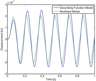
. (11) Figure 11 shows simulations of the model utilizing the describing and the nonlinear model for a sinusoidal force input at a frequency equal to ωd. Bipolar displacement will not reliablyoccur at frequencies greater than this value. This is very clearly observed in the nonlinear model. With the values used in the simulations, 2ωd has a value of 77.5 rad/s. Keep in mind that
when bipolar displacement occurs, the input frequency of the actuators is twice that of the output displacement frequency. Thus, we should expect bipolar output displacements to be unstable at frequencies higher than approximately 77.5 rad/s. We see this clearly in the simulations shown in Fig. 12. The driving frequency of 76 rad/s produces clean clear bipolar oscillations once transient effects of initial conditions attenuate. Conversely, the driving frequency of 77 rad/s produces erratic, unpredictable passes through the singularity point. Thus, it is clear that the model derived using the describing function method is accurate in determining the upper bound on the frequency band of reliable bipolar oscillations.
0 0.2 0.4 0.6 0.8 1 -3 -2 -1 0 1 2 3x 10 -3 Time [s] D isp la ce m e n t [ m ]
Describing Function Model Nonlinear Model
FIGURE 11. SINUSOIDAL FORCE INPUT RESPONSE OF THE NONLINEAR MODEL AND THE MODEL LINIARIZED VIA THE
DESCRIBING FUNCTION METHOD AT THE DAMPED NATURAL FREQUENCY OF THE LINEARIZED MODEL
0 0.5 1 1.5 -2.5 -2 -1.5 -1 -0.5 0 0.5 1 1.5 2 2.5 Time [s] D is p la ce me n t y [mm]
76 rad/s Driving Frequency
0 0.5 1 1.5 -2.5 -2 -1.5 -1 -0.5 0 0.5 1 1.5 2 2.5 Time [s] D is p la ce me n t y [mm]
77 rad/s Driving Frequency
FIGURE 12. NONLINEAR MODEL DRIVEN BY PZT STACKS AT 76 RAD/SEC (LEFT) WITH PERFECT RELIABLE BIPOLAR
OPERATION AND 77 RAD/SEC (RIGHT) WITH SPORADIC UNRELIABLE BIPOLAR OPERATION
We now have intuitive values that define the frequency band at which bipolar displacement will occur. The lower bound is defined by the frequency at which the linear model from Eq. (5) predicts displacements reaching near the singularity point, and the frequency from Eq. (11) predicts the frequency at which bipolar displacement will no longer be sustained. These tools should be used in the design process to quickly and accurately mach the frequency band of the actuator to the frequency requirement of the application. Once more precision is required, the more physically realistic nonlinear model should be used.
FIGIGURE 13. DYNAMIC MOTION PROTOTYPE THAT PASSES THROUGH SINGULARITY POINT CAPABLE OF
2.44 MM OF DISPLACEMENT AT 32 HZ 0 0.02 0.04 0.06 0.08 0.1 0 0.5 1 1.5 2 2.5 Time [s] D is pla ce me nt [ mm]
FIGURE 14. INPUT SQUARE WAVE SIGNAL AND OUTPUT RESPONSE OF PLASTIC ACTUATOR DYNAMICALLY PASSING THROUGH THE SINGULARITY
POINT
EXPERIMENTAL PROTOTYPES AND RESULTS
Multiple prototypes where fabricated and tested to study the three modes of output displacement described above. One is made out of an ABS based plastic using a dimension sst 1200es 3D printer[14]. It is shown in Fig. 13. It was valuable for testing because the series stiffness, k, as depicted in Fig. 2, was small and allowed for great magnitudes of displacement. Weights were attached to the output node along the output axis to test the drivability of different loads and observe the effects on the frequency response. The low and high frequency mono-polar modes were trivially reproduced, while the bipolar mode was only generated within the predicted frequency range. At the optimal mass load, the plastic device oscillated stably at 32 Hz (actuated at 64 Hz) with a displacement magnitude of 2.44 mm. This displacement is greater than 150 times the displacement provided by the input PZT actuator (18 μm). The displacement profile of this is shown in Fig. 14.
Another prototype fabricated and tested is made out of steel and is shown in Fig. 15. The flexures were machined via electric discharge machining (EDM) and the preload length, lp, was
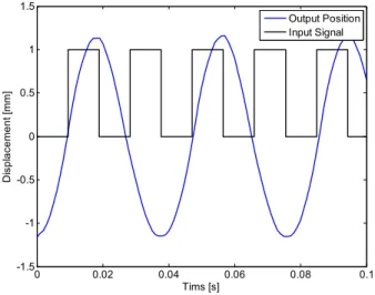
adjusted by filing the contact points of the PZT stacks. This prototype is much stiffer than the previous. This allows for faster oscillations, larger loads and greater output force. The peak force is 10.8 N. With the optimal mass load, bipolar oscillations were achievable at 53 Hz, with a displacement magnitude of 2.37 mm as shown in Fig. 16.
PZT Stacks Rigid Frame Output Axis
FIGURE 15. PROTOTYPE THAT PASSES THROUGH SINGULARITY POINT CAPABLE OF 2.37 MM OF DISPLACEMENT AT 53 HZ, AND MEASURED FORCE OF
10.8 N 0 0.02 0.04 0.06 0.08 0.1 -1.5 -1 -0.5 0 0.5 1 1.5 D is p la cem ent [m m ] Tims [s] Output Position Input Signal
FIGURE 16. INPUT SQUARE WAVE SIGNAL AND OUTPUT RESPONSE OF STEEL ACTUATOR DYNAMICALLY PASSING THROUGH THE SINGULARITY
POINT
CONCLUDING REMARKS
In this paper we have presented the buckling actuator concept and provided a framework with which to utilize it dynamically within specific applications. There is a well defined frequency band at which bipolar, large displacement occurs. Using the linearized models presented, the band can be easily and intuitively tuned. Using the more complex, less intuitive nonlinear model, the performance of specific designs can be evaluated precisely.
Dynamically operating piezoelectric actuators are already frequently used. In commercially available actuators, some utilize taking small steps, while others utilize deforming a rigid material to generate moving waves [2]. Our dynamically activated buckling actuator provides performance in the design space between frequency leveraged displacement amplification actuators, and geometrically leveraged displacement amplification actuators. By utilizing the buckling actuator within an optimal frequency band, the output displacement and transfer of power to the load can be maximized and applied to macro scale applications.
Future research efforts will utilize multiple buckling actuators in parallel, operating within the optimal frequency band to drive a single load.
REFERENCES
[1] Niezrecki, C., Brei, D., Balakrishnan, S., Moskalik, A. 2001. “Piezoelectric Actuation: State of the Art,” The Shock and Vibration Digest, 33 (4), pp. 269-280. [2] Physik Instrumente, Piezo Nano Positioning Inspirations
2009.
[3] Touli, W., 1966 “Flexural-extensional electromechanical transducer,” US Patent 3,277,433.
[4] Newnham, R., Dogan, A., Xu, Q., Onitsuka, K., Tressler, J., Yoshikawa, S., 1993 “Flextensional Moonie Actuators,” In 1993 IEEE Proceedings. Ultrasonics Symposium, vol. 1, pp. 509–513.
[5] Dogan, A., Uchino, K., Newnham, R., 1997. “Composite piezoelectric transducer with truncated conical endcaps ‘Cymbal’,” IEEE Transaction on Ultrasonics,
Ferroelectricsand Frequency Control, vol. 44, no. 3, pp. 597-605.
[6] Onitsuka, K., Dogan, A., Tressler, J., Xu, Q., Yoshikawa, S., Newnham, R., 1995. “Metal-Ceramic Composite Transducer, the ‘Moonie’,” Journal of Intelligent Material Systems and Structures, vol. 6, no. 4, p.447.
[7] Ueda, J., Secord, T., Asada, H., 2008. “Static lumped parameter model for nested PZT cellular actuators with exponential strain amplification mechanisms," in IEEE International Conference on Robotics and Automation, pp. 3582-3587.
[8] Wingert, A., Lichter, M., Dubowsky, S., 2002. “Hyper-Redundant Robot Manipulators Actuated by Optimized Binary Dielectric Polymers,” in Proceedings of SPIE, vol. 4695, pp. 415-423.
[9] Neal, D., Asada, H., 2009. “Nonlinear, Large-Strain PZT Actuators Using Controlled Structural Buckling,” in Proceeding of the IEEE International Conference on Robotics and Automation, pp 3677-3682.
[10] Neal, D., Asada, H., 2010. “Phased-Array Piezoelectric Actuators Using a Buckling Mechanism Having Large Displacement Amplification and Nonlinear Stiffness,” Proceeding of the IEEE International Conference on Robotics and Automation, to be published.
[11] Thorlabs.com, “Piezo-electric actuators," August 2009. [12] Neal, D., Asada, H., 2008. “Design of Cellular
Piezoelectric Actuators With High Blocking Force and High Strain,” Proceedings of ASME Dynamic Systems and Control Conference.
[13] Slotine, J., Li, W., 1991. Applied Nonlinear Conrol, 1st ed.
Prentice-Hall, Englewood Cliffs, New Jersey, Chap. 5, pp 159-171.
[14] www.dimensionprinting.com, “3D Printers: Dimension 1200 Series Specs," March 2010.
PZT Stacks Rigid Frame Output Axis