Digital image warping : theory and real time hardware implementation issues

Digital Image Warping:

Theory and Real Time Hardware Implementation Issues

by

Mark Sebastian Lohmeyer

Submitted to the Department of Electrical Engineering and Com-puter Science in Partial Fulfillment of the Requirements for the Degrees of Bachelor of Science in Electrical Science and

Engineer-ing and Master of EngineerEngineer-ing in Electrical EngineerEngineer-ing and Com-puter Science

at the

MASSACHUSETTS INSTITUTE OF TECHNOLOGY

© 1996 Mark S. Lohmeyer. All Rights Reserved.

The author hereby grants to M.I.T. permission to reproduce distrib-ute publicly paper and electronic copies of this thesis and to grant

others the right to do so.

Author ...

Department ot Electrical Engmeerntg anau , mputer Science May 17, 1996 Certified by ... George Verghese Thesis Supervisor :. Morgenthaler ,raduate Theses Accepted by

1;ASSACHUSE fTS INIST'fU i'E

OF TECHNOLOGY

JUN

1

1 1996

Digital Image Warping:

Theory and Real Time Hardware Implementation Issues

Mark Sebastian Lohmeyer Submitted to the

Department of Electrical Engineering and Computer Science May 17, 1996

In Partial Fulfillment of the Requirements for the Degree of Bache-lor of Science in Electrical Science and Engineering and Master of

Engineering in Electrical Engineering and Computer Science

Abstract

This thesis begins with a broad introduction to digital image warping. It includes back-ground on spatial transformations and basic signal processing theory as they are used in the warping application. Next, an analysis of various interpolation kernels in the time domain is performed. The results from this study lead directly to a new approach to per-forming a generalized high-quality image warp that maps well to an efficient hardware implementation. Finally, the design of a hardware system capable of performing image warps in real-time is described.

Thesis Supervisor: George Verghese

Acknowledgments

First I would like to thank my 6-A internship company, the David Sarnoff Research Center for sponsoring my work. In particular, I would like to recognize Gooitzen van der Wal and Peter Burt for finding me such an interesting project, supervising my work, and always having the time to listen and help.

Thanks to Professor George Verghese for being my MIT thesis supervisor and providing great feedback throughout the process.

Thanks to my family for always being so supportive (and keeping me well supplied with candy and cookies.)

Thanks to my brother Dan for always using my car so I had nothing else to do but work on my thesis.

Thanks to all my friends at MIT for providing me with plenty of opportunities to relax and take my mind off of thesis.

Finally, thanks to Benjie Chen for providing me with disk space to store all those warped images.

Table of Contents

1 Introduction ... 13

1.1 Im age W arping... ... 13

1.2 Thesis Overview ... 14

2 Spatial Transform ations ... ... 17

2.1 D efinitions... 17

2.2 Polynomial Transformations... ... 18

2.3 Perspective Transformation ... 19

2.4 Flow-Field Transformation ... 20

2.5 Summary Remarks ... ... 20

3 Resampling Theory for Image Warping ... 23

3.1 Sampling of Continuous-Time Signals ... .... 23

3.2 Resampling Through Interpolation in Digital Domain... 28

3.3 Summary Remarks... ... 33

4 Analysis of Interpolation Methods for Image Resampling... ... 35

4.1 D escription ... 35

4.2 Expected Error Calculation... ... 36

4.3 Sampling Rate Issues ... 41

5 High Quality, Efficient Image Warping...45

5.1 General Description of Method. ... 45

5.2 Comparison with Standard Techniques ... ... 53

5.3 Optimal Upsampling Kernel Design... ... 61

5.4 Final R em arks ... ... 73

6 H ardw are D esign ... ... 75

6.1 B ackground ... ... 75

6.2 Functionality Requirements ... 75

6.3 C om ponents ... ... 75

6.4 High-Level Design ... ... 77

6.5 Warp Board Functional Description ... ... 77

6.6 Warp Control Block... ... 78

6.7 Address Generation Block ... 82

6.8 Warp Memory Block ... ... 83

6.9 Coefficient Look-Up Table ... 84

6.10 Sum of Products Interpolator ... 85

6.11 C onclusion ... ... 86

7 C onclusions... ... 87

7.1 Summary of Work... ... 87

7.2 Further Research ... ... 87

Appendix A Forward Difference Method ... 89

List of Figures

Figure 2.1: General inverse mapping ... ... 17

Figure 3.1: Continuous signal to discrete signal ... ... 24

Figure 3.2: Continuous signal to discrete signal in the frequency domain ... 27

Figure 3.3: Resampling at an arbitrary location... 30

Figure 3.4: Upsampling by U in frequency domain. ... ... 32

Figure 3.5: Downsampling, with and without aliasing ... 33

Figure 4.1: Reconstruction error illustration... 37

Figure 4.2: Interpolation kernels and their frequency responses ... 38

Figure 4.3: Expected error vs. frequency for sampling rate of 2000Hz. ... 39

Figure 4.4: Expected error vs. frequency for sampling rate of 2000Hz. ... 40

Figure 4.5: Sampling rate multiplier (linear vs. cubic convolution) ... 42

Figure 4.6: Sampling rate multiplier (nearest neighbor vs. linear) ... 42

Figure 5.1: High quality warp system ... ... 46

Figure 5.2: Upsampling stage ... 48

Figure 5.3: Frequency domain comparison. ... ... 49

Figure 5.4: Downsampling as part of image warp ... ... 50

Figure 5.5: Original and bilinear rotation images... ... 56

Figure 5.6: Keys-3 and Keys-4 rotation images. ... ... 56

Figure 5.7: Up2(Keys-3) and Up2(Keys-4) rotation images ... 57

Figure 5.8: Diamond cycle RMS error. ... 58

Figure 5.9: Diamond cycle RMS error. ... ... 59

Figure 5.10: Original and bilinear after 12 diamond cycles. ... 60

Figure 5.11: Keys-3 and Keys-4 after 12 diamond cycles ... 60

Figure 5.12: Up2(Keys-3) and Up2(Key-4) after 12 diamond cycles ... 61

Figure 5.13: General 4 tap upsampling filter ... ... 63

Figure 5.14: Frequency response of various 4-tap filters. ... 63

Figure 5.15: Frequency response of overall system for integer and half-pixel translation us-ing the Lohmeyer kernel for upsamplus-ing ... 65

Figure 5.16: Frequency response of overall system for integer and half-pixel translations using Pyramid kernel for upsampling ... ... 66

Figure 5.17: Up2(Loh) and Up2(Pyr) images after 16 rotations. ... 67

Figure 5.18: RMS error for diamond test...68

Figure 5.19: RMS error for diamond test...68

Figure 5.20: Up2(Loh) and Up2(Pyr) for diamond test ... 69

Figure 5.21: RMS error for random translation test. ... ... 70

Figure 5.22: RMS error for random translation ... ... 70

Figure 5.23: Original and bilinear image ... 71

Figure 5.24: Keys-3 and Keys-4 images ... 72

Figure 5.25: Up2(Keys-3) and Up2(Keys-4) images...72

Figure 5.26: Up2(Loh) and Up2(Pyr) images ... 73

Figure 6.1: Warp module block diagram. ... ... 76

Figure 6.2: Image data timing ... ... ... 80

List of Tables

Table 5.2; RMS Error for Rotation 55 Table 5.3: RMS Error for Rotation 66 Table 6.1: Warp Board Inputs 77 Table 6.2: Warp Board Outputs 77 Table 6.3: Control Registers 79 Table 6.4: Write Process 80 Table 6.5: Read Process 82 Table A.1: Increment Table 89

Chapter 1

Introduction

1.1 Image Warping

Digital image warping is an important and expanding branch of the field of digital image processing. In general, a digital image warp is a geometric transformation of a digitized image. Simple examples of warps include translation, rotation, and scale change. More complex warps can apply an arbitrary geometric transformation to the image.

Image warping was first used extensively for geometric correction in remote sensing applications. In the past twenty years, the field has grown to encompass a broad range of applications. These include medical imaging, image stabilization, machine vision, image synthesis and special effects generation. Every application has different speed, accuracy, and flexibility requirements. For example, the warping for movie special effects has to result in high-quality video, but the frames can be processed off-line and then pasted together into a sequence afterwards. On the other hand, in certain machine vision applica-tions, the warping must occur in real-time, but the quality of the resultant warped images is not as critical.

In recent years, with the advances in digital logic and memory, it has become possible to perform many image processing tasks in real-time on specialized hardware. Image warping is no exception. There is a wealth of applications where real-time image warping is required. Moving target detection from a moving platform is one example. In this case, it is not adequate to simply detect motion by frame differencing because the motion due to the target will be lost in the motion from the moving camera. Instead, if the frames are first warped to remove the motion due to the camera, and then differenced, the only motion left will be due to the target. This motion can then be detected more readily. The desire to

per-form image warping in real-time has lead to an increased interest in algorithms that map well to an efficient hardware implementation.

There are two basic components to an image warp: spatial transformation and resam-pling through interpolation. A spatial transformation defines a geometric relationship between each point in the input image and a corresponding point in the output image. There are many possible models for this geometric relationship. Typically, the spatial transformation will require the value of points in the source image that do not correspond to the integral sample positions. This is where the second component of image warping, namely age resampling through interpolation, becomes important. Some sort of interpola-tion is required to estimate the value of the underlying continuous source image at loca-tions that don't correspond to the sample points. Together, these two components determine the type and the quality of the warp.

1.2 Thesis Overview

This thesis begins with a broad introduction to image warping. Background on spatial transformations and basic signal processing theory are introduced to the extent required in the warping application. Next, an analysis of various interpolation kernels in the time domain is performed. The results from this study lead directly to an interesting approach to performing a generalized high-quality image warp that maps well to an efficient hard-ware implementation. Finally, the thesis describes the design of a hardhard-ware system capa-ble of performing image warps in real-time.

The thesis is divided into chapters as follows: Chapter 1 is an introduction to image warping.

Chapter 2 gives background on spatial transformations. There are many ways to spec-ify the relationship between points in the source and target images. Different

representa-tions allow for varying degrees of freedom. The price for greater freedom is often higher computational complexity. These trade-offs are analyzed, particularly in terms of their mapping to an efficient hardware implementation. Three transformations are described in some detail because they are each important for certain real-time machine vision tasks. These are: the polynomial transformation, the perspective transformation, and the flow-field transformation.

Chapter 3 gives the theoretical framework for image resampling. First it discusses sampling of continuous-time signals. Next it examines how a continuous signal can be reconstructed from its samples with a low-pass filter and then resampled to form a new discrete sequence. Finally, this chapter reviews aliasing within the image warping frame-work and discusses how it may be avoided through preprocessing.

Chapter 4 is an analysis of methods of resampling through interpolation. First, it describes some candidate interpolation kernels for resampling. Then it analyzes their per-formance in the time domain. For each interpolation method, and a specified sampling rate, the expected error between an original and reconstructed sinusoid of a certain fre-quency is calculated. The error is then computed and graphed for a wide range of frequen-cies to determine how the interpolation method performs as a function of the frequency of the original signal. Next, the sampling rate is allowed to vary, while the frequency of the analog sinusoid is fixed. In this way, it is possible to determine how much the sampling rate must increase for an otherwise poor interpolation method to perform adequately. The results of Chapter 4 lead directly to an interesting method of performing an image warp, which may have numerous advantages over some previous approaches. This method is analyzed in Chapter 5.

Chapter 5 describes a method for performing high quality, computationally efficient digital image warping through upsampling followed by warping and downsampling using

a smaller kernel for interpolation. This approach makes it particularly suitable for a low-complexity hardware implementation. Next, the performance of this algorithm is tested under a variety of conditions on actual images, and compared to standard techniques. Finally, based on the test results and knowledge of the filter used in the warping stage, an attempt is made to select an optimal filter for the upsampling stage.

Chapter 6 describes the hardware design of a specific warper implementation for use in a real-time image processing system. This includes a block diagram, summary of com-ponents, and board level design description. The chapter also analyzes the engineering

trade-offs encountered in the design.

Chapter 7 is a summary of the work completed, and a discussion of topics for further research.

Chapter 2

Spatial Transformations

2.1 Definitions

In a digital image warp, the spatial transformation defines a geometric relationship between each point in the input or source image and its corresponding point in the output or target image [13]. This relationship between the points can be specified as either a for-ward or inverse mapping. If [u,v] refers to the input image coordinates and [x,y] refers to the output image coordinates, then a forward mapping gives the locations [x,y] as some function of [u,v]. Likewise, an inverse mapping gives [u,v] as a function of [x,y]. This is depicted in Figure 2.1, where U and V are the inverse mapping functions. For most hard-ware implementations, the inverse mapping is a more appropriate representation.

The inverse mapping specifies reference locations in the source image as a function of the current location in the target image.

u x

V

y

0

Source Image

Target Image

[u,v] = [U(x,y), V(x,y)]

Commonly, the locations in the target image are sequentially stepped through, and at each integer position the reference location in the source image is calculated. Because the inverse mapping function can be arbitrary, the referenced source location may not have integer coordinates. Therefore, some sort of interpolation is required to give the input value at nonintegral input locations. This will be discussed later. The second difficulty with the inverse mapping is that pixels in the source image may be left unaccounted for in the target image. If the input is not appropriately bandlimited prior to this sort of a map-ping, aliasing can occur. Methods of avoiding this aliasing will also be discussed later.

In this chapter, three general categories of inverse mappings will be presented. These are: polynomial, perspective, and flow-field transformations. The selection of the most appropriate model depends upon both the application and the implementation require-ments. The models will be discussed in these terms.

2.2 Polynomial Transformations

The polynomial inverse transformation is usually given in the form

N N u = _ _a(i,j) x i i = Oj = 0 N N v = I b (i,j)x '_iy i = Oj = 0 Polynomial transformation (2.1)

where a(i,j) and b(i,j) are constant coefficients. This transformation originated in the remote sensing field, where it was used to correct both internal sensor distortions and external image distortions. It is currently being used in a wide range of applications. Mosaic construction is one example [5]. Typical hardware implementations use the

for-ward differencing method to compute [u,v]. This is discussed in Appendix A.

One specific polynomial transformation that is commonly used is the affine transfor-mation, specified as

u = a+bx+cy v = d+ex+fy

Affine transformation (2.2)

This transformation allows for image translation, rotation, scale, and shear. It has six degrees of freedom, given by the six arbitrary constants. Therefore, only three correspond-ing points in a source and target image are needed to infer the mappcorrespond-ing. The affine trans-formation can map a triangle to any other triangle. It can also map a rectangle to a parallelogram. It cannot, however, map one arbitrary quadrilateral into another.

The affine transformation is particularly well suited for implementation in hardware using the forward differencing method. Using the forward differencing method to calcu-late the source image addresses requires six registers to hold the values of the constant coefficients, four accumulators to store and update the current reference address, and four two-to-one multiplexers to pipe the correct increment values to the accumulators.

2.3 Perspective Transformation

The inverse mapping function of a perspective transformation is given as

a + bx + cy e +fx + gy h + ix + jy e +fx + gy

Perspective transformation (2.3)

transformation. Iff and g are not zero, then it is a perspective or projective mapping. The perspective mapping preserves lines in all orientations. The perspective mapping has eight degrees of freedom, which permits arbitrary quadrilateral-to-quadrilateral mappings.

Because the perspective transformation requires a division, it is not as easy to imple-ment in hardware as the affine transformation. The numerator and denominator for each [u,v] value can be computed using the forward differencing method, just as in the affine case. Then a division is needed. This could be performed in a specialized division chip, which may introduce a fairly long pipeline delay. Or, it could be done in a large look-up table. Depending on the required accuracy of the result, both of these methods may be pro-hibitively expensive in terms of cost or space. The perspective transformation can also be approximated by a polynomial transformation of high enough order. In many applications, a second or third degree polynomial will be adequate.

2.4 Flow-Field Transformation

The flow-field transformation is the most general transformation. It can be used to realize any other spatial mapping. It can be viewed simply as a table that gives an input location to reference for each output location. If these flow-field values are given to the warper module from other modules, the flow-field adds very little complexity to the warper mod-ule. The trade-off, of course, is that significant resources may be required elsewhere to compute these flow-field values.

2.5

Summary Remarks

This is only a brief description of some common spatial transformations, focusing on those transformations that are being considered for real-time hardware implementation at the David Sarnoff Research Center. A more detailed description of these and other geo-metric transformations can be found in [13]. A related problem is the estimation of the

constants of the warp equation, given a set of constraints. For example, in performing image stabilization, interframe motion must be accurately estimated. It has been shown that a multiresolution, iterative process operating in a coarse-to-fine fashion is an efficient way to perform this estimation. During each iteration, an optical flow-field is estimated between the images through local cross-correlation analysis, then a motion model is fit to the flow-field using weighted least-squares regression. The estimated transform is then used to warp the previous image to the current image and the process is repeated between them, [5]. This and other methods of estimating the warping parameters will not be dis-cussed in further detail here.

Chapter 3

Resampling Theory for Image Warping

3.1 Sampling of Continuous-Time Signals

Digital images are created by a variety of means. These fall into two general categories: computer-generated images and sampled images. Computer-generated graphics assign pixel values based on a mathematical formula. This can range from something as simple as a two-dimensional graph to a complex animation program derived from the laws of physics. If such a mathematical model is available, it is appropriate to warp the image

sim-ply by evaluating the formula at different points. In the case of sampled images, however,

no such formula is available. Usually, all that is available is the actual samples. To under-stand what can be done under these conditions, one must underunder-stand the digital image as a representation of a continuous image in both the spatial and frequency domains. First, the one-dimensional case is examined.

The discrete representation of a continuous signal is usually obtained by periodically sampling the continuous signal. If the sampling rate is T, this relationship is expressed as:

f[n] = fc (nT)

(3.1)

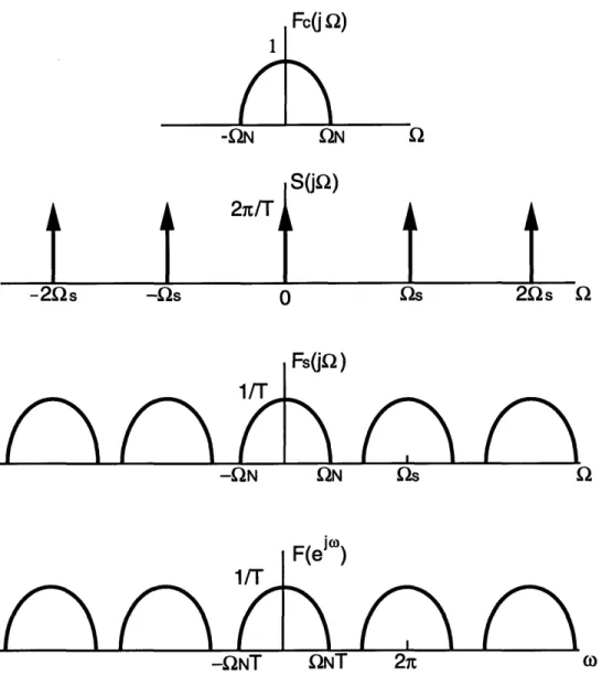
To derive the relationship between the Fourier transforms off[n] andfc(x), it is helpful to analyze this conversion in two steps. In the first step, the continuous signal is sampled by multiplication with an impulse train of period T. The second step is to then convert this impulse train into a discrete sequence. This process is shown in the spatial domain in Fig-ure 3.1.

S(X)

S.LILLLUI

Figure 3.1: Continuous signal to discrete signal.

The impulse train of period T can be written mathematically as:

s(x) =

B ((x-nT)

fs (x) = fc (x) s (x)

Since fs(x) is the product offc(x) and s(x), the Fourier transform offs(x) is the convolution of the Fourier transforms offc(x) and s(x):

Fs (jQ) = Fc (jQ) *S (jQ)

(3.5) The Fourier transform of s(x) is:

sO(jn) =

k = -00

where Qs= 21i/T, which is the sampling frequency. Doing the convolution then gives:

fc(x)

(3.6)

Fs (j) = Fc (j - kjs) (3.7)

Equation 3.7 gives the frequency-domain relationship between the original analog sig-nal and the impulse-sampled asig-nalog sigsig-nal. The Fourier transform of the impulse sampled signal comprises copies of the Fourier transform of the original signal superimposed at integer multiples of the sampling frequency. The higher the sampling rate, the further these copies are spread apart. From this analysis, one can see the origins of the Nyquist Sampling Theorem. If the original analog signal is bandlimited, it is possible to sample at a high enough rate that the copies of the Fourier transform of the original signal do not overlap in the Fourier transform of the sampled signal. If there is no overlap, then the orig-inal signal can be exactly reconstructed with an ideal lowpass filter with the correct gain. An ideal lowpass filter will reject all copies except the one centered at the origin, giving the original signal back. For there to be no overlap, the sampling rate must be at least twice the maximum frequency component of the original signal:

Us > 2Mn

(3.8)

If there is overlap in the frequency domain, the signal can no longer be exactly recon-structed from its samples. The error that occurs due to this overlap is referred to as alias-ing.

The second step in the continuous to discrete process is the conversion from the impulse-sampled signal in the continuous domain to a discrete sequence. The values of the discrete time sequence at n = 0, 1, 2,... are the areas of the impulses at 0, Us, 2Ms,... But what does this do in the frequency domain?

First the results will be derived mathematically. Taking the Fourier transform of equa-tion 3.4 gives:

Since Fs (jf) = fc (nT) e-jaTn fn] = -fc(n f [n] fc (nT) and F (eJi) = f [n] e-jon n = -0

looking at Equations 3.9, 3.10, and 3.11, it can be seen that

Fs (jQ) = F(ei•)

I

Now, from Equations 3.7 and 3.13.

1 oo

F(ejQT)

=

1

- F

_(jQ-jkQs)

k = -oo

(3.13) which can also be written

1 .co .2·rk •

F (eJ(O)

F

2-)

(3.14)

k = -0W

From these equations it can be seen that the conversion from the continuous domain train of impulses to a discrete sequence corresponds to a rescaling of the frequency axis in the frequency domain. The frequency scaling is given by cow=T. This scaling normalizes the continuous frequency 9=Qs to o-=2t for the Fourier transform. This makes some intu-itive sense as well. In the spatial domain, the impulses are spaced T apart, while the dis-crete sequence values are spaced apart by one. Thus, the spatial axis is normalized by a factor of T. In the frequency domain then, the axis is normalized by a factor of 1/T. [10]

(3.9)

(3.10)

(3.11)

A graphical representation is quite useful in understanding the relationship between all these signals. This is shown in Figure 3.2.

FP/ti 01 S(jQ)

i

-ON

ON

Qs

Q

1/T

Figure 3.2: Continuous signal to discrete signal in the frequency domain.

The whole continuous-to-discrete sampling process can be summarized quite simply in the spatial and frequency domain. In the spatial domain, the values of the discrete sequence at n = 0, 1, 2, etc. are the values of the continuous-time signal at the sample

points, 0, T, 2T, etc. In the frequency domain, the Fourier transform of the discrete sequence can be produced by normalizing the frequency axis of the continuous signal by a factor of 1/T, and then replicating this at all integer multiples of 27t. The two-dimensional case can be analyzed using the same methods as in the one-dimensional case here. The only difference is now one has to worry about frequencies in two dimensions.

For the purposes of this thesis, it will be assumed that no appreciable aliasing occurs in the continuous to discrete sampling of an image. This is indeed the case with most of the images encountered in typical image warping applications. However, understanding the relationships between the underlying analog image and its samples is still of extreme importance for warping. In this situation, a discrete image is all that is given. The values of the underlying continuous image are only known at integer locations in this discrete image. If this image is then to be warped based on a geometric transformation, it is very probable that the values of the continuous image at other positions than the original sam-ple points will be needed. This is the fundamental resampling problem encountered in dig-ital image warping.

3.2 Resampling Through Interpolation in Digital Domain

Resampling is the process of transforming a digital image from one coordinate system to another. In the case of image warping, these two coordinate systems are related to each other by the spatial transformation that defines the warp. Conceptually, resampling can be divided into two steps. First, interpolate the discrete image into a continuous one. Second, sample this continuous image at the desired locations to form the resampled image. In practice, these two steps are often consolidated so the interpolated values are only calcu-lated for those locations that will be sampled. This makes it possible to implement the res-ampling procedure entirely in the digital domain. This section discusses the spatial and frequency-domain interpretations of the resampling process. It also examines how this

res-ampling can be accomplished in digital hardware for an arbitrary geometric transforma-tion functransforma-tion.

Conceptually, the first step in the resampling process is reconstruction of the bandlim-ited analog signal from its samples. In Section 3.1, it was shown that if the original signal after modulation by an impulse train was appropriately low-pass filtered, it would return the original analog signal. This impulse train, fs(t), can be constructed from the discrete samples as follows:

fs(x) = f[n] 8 (x-nT) (3.15)

n = -oo

Then if Hr(jQ) is the frequency response of the low-pass filter, and h,(x) is its impulse response, the reconstructed signal at the output of the filter is:

fr(x) = f[n]hr(x-nT) (3.16)

n = -oo

The perfect Hr(jI) is an ideal low-pass filter with cut-off frequency of R/T and a gain of T. In the spatial domain, this is a sinc function:

sin(

mc)

hr(x) = (3.17)

7Cx T

So, perfect reconstruction comes from convolving the samples with a sinc function. One important property of this sinc function is that it has a value of unity at x=O, and a value of zero at all other integer multiples of T. This means that the reconstructed signal has the same values at the sample points as the original continuous signal.

After the continuous signal is reconstructed, it can be resampled at different positions to form the resampled sequence. Of course, in real implementations, this is not how the resampling is performed. One approach to performing this resampling entirely in the digi-tal domain is discussed below.

In the typical resampling problem, the samples at integer locations are given. From these, we wish to determine the value of the continuous sequence at other locations. This

is shown in Figure 3.3.

f rn f c(x) "

Figure 3.3: Resampling at an arbitrary location.

It is obvious at this point that the sinc function can not possibly be used for reconstruc-tion, as it is infinitely long. Instead, a finite length interpolation function must be used so that the convolution can be performed. Of course, this means that it will not correspond to a perfect low-pass filter, which will result in some error. The trade-offs involved in picking an appropriate interpolation method are discussed in greater detail in Chapter 4. For prac-tical implementations, a interpolation kernel of finite length is used. To demonstrate the approach, a kernel with a width of four will be used. This interpolation kernel will be

referred to as hr4(x).

Call the spatial location we are interested in loc. This can be written as the sum of a fractional and an integer part:

loc = intloc +fracloc (3.18)

So if loc is 2.3, intloc is 2 andfracloc is 0.3. Now, it can be seen that if the convolution was carried out using hr4(X) as the kernel, the value of the function at loc would be:

2

fr (loc) = C f[k +intloc] x hr4 (fracloc-k) (3.19)

k= -1

This approach lends itself well to a hardware implementation. A look-up table can be used to store the values of the interpolation kernel. The integer portion of the referenced source location is used to determine which sample points are accessed, and the fractional part of the source location determines the weights of the coefficients as generated by the look-up table. The final value at the referenced location is given by a sum of products of the sample points and the weighting coefficients. This approach can easily be used in two dimensions for image warping resampling. For example, if the one dimensional interpola-tion kernel is of width four, then this method will require a pixel area of 4x4, with sixteen weighting coefficients.

Next, it will be helpful to examine the effects that upsampling and downsampling have in the frequency domain. In general, the geometric transform of an image warp may require upsampling in some areas of the image and downsampling in others. Or, it may simply require a shift, which is neither upsampling or downsampling. The frequency-domain interpretation of such arbitrary resampling is difficult to represent in closed math-ematical form. Therefore, it will be useful to analyze the simpler cases of regular upsam-pling and downsamupsam-pling to gain intuition into the frequency-domain effects of the resampling required by a geometric transformation. In this analysis, it will be assumed that the interpolation uses an ideal low-pass filter. If this is the case, then resampling in the

Upsampling refers to an increase in the sampling rate. For example, upsampling by two corresponds to doubling the sampling rate of the continuous signal. From the analysis in Section 3.1, it can easily be seen that upsampling corresponds to a compression of the Fourier transform. If the signal in upsampled by a factor of U, then the Fourier transform is compressed in frequency by that same factor. This is shown in Figure 3.4.

IHl(eJ0)l _{IH2(ej0 )}

Upsampling

-2c -1_ C 27 -2n -itU iM/U 2n

Figure 3.4: Upsampling by U in frequency domain.

Of course, the relationship above holds only if the low-pass filter used for interpolation is

ideal; if it is not ideal, then some distortion will occur.

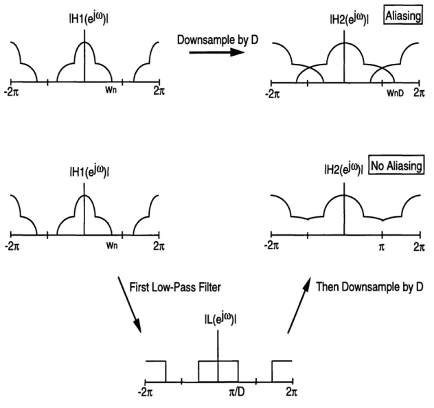
Downsampling refers to a decrease in the sampling rate. If the signal is not appropri-ately low-pass filtered before the downsampling occurs, aliasing can result. If the signal is downsampled by a factor of D, then the Fourier transform of the signal is expanded in fre-quency by that same factor. This can lead to an overlap in the frefre-quency domain, which is the cause of the aliasing. The problem is identical to that of sampling the original continu-ous signal below the Nyquist rate. This aliasing problem can be avoiding by pre-filtering the signal with a discrete-time low-pass filter to remove the frequencies that would over-lap, as shown in Figure 3.5.

IH1(ejW)Il

IH1(ejW)I)

IH2(eJ)l

IAliasingI

Downsample by D

lH2(eJ)Il

INo

Aliasingi

First Low-Pass Filter

IL(eJ)Il

/

Then Downsample by D

n/D

Figure 3.5: Downsampling, with and without aliasing.

3.3 Summary Remarks

In practice, for machine vision applications, aliasing usually is not a severe problem. The geometric transformations rarely requite shrinking the image to a size where aliasing might result. Also, the frequency composition of typical images rarely contains much energy in the higher frequencies that would overlap. For example, if the image contains no energy in radian frequencies higher than 7c/2, then the image can be downsampled by a

rt

2

factor of two in both directions, and no aliasing will occur. Also, if the geometric transfor-mation is known beforehand, then the image can be preprocessed with a low-pass filter to remove the frequencies that would cause problems. Methods of performing this pre-filter-ing will not be discussed in further detail here.

The usual culprit in poor quality image warps comes not from aliasing, but from the method used for interpolation prior to resampling. Chapter 4 will analyze the performance of some interpolation kernels, and discuss the implications of the results.

Chapter 4

Analysis of Interpolation Methods for Image

Resam-pling

4.1 Description

The real problem to be analyzed here is how well a continuous image can be recon-structed from its samples using practical interpolators. If the original continuous image is bandlimited and sampled above the Nyquist frequency, sampling theory shows it can be exactly recovered with a perfect low-pass filter. In the spatial domain, this corresponds to convolving with a two dimensional sinc function. This is not a practical option, as the sinc function is infinitely long and falls off only as the reciprocal of distance. Instead, practical implementations use an interpolation kernel of finite support. In general, the larger the support of the interpolation kernel is allowed to be, the more accurately its frequency response can approximate the ideal. However, longer interpolation kernels require greater computational resources to implement. This is the fundamental trade-off: efficient compu-tation versus accuracy of reconstruction. Much work has been done to identify methods of interpolation that strike an appropriate balance between these two competing require-ments.

There are numerous papers that compare various interpolation methods for their accu-racy of reconstruction [8]. Two general approaches to evaluation are usually taken. The first is simply to resample test images using different interpolation methods and visually assess the quality of the resultant image. The second, more analytical method is to base the evaluation on the frequency characteristics of the interpolation kernel.

The first method is very straightforward, and appropriate for applications where dis-play for human viewing is the ultimate goal. It has the natural advantage that it includes

the effects of human perception. However, it is somewhat ad hoc; the error is not quanti-fied. For comparison of interpolation methods, all that can really be said is that one "looks" better that the other. What may be reasonable for viewing may not be adequate if further calculations are to be performed.

The second method, on the other hand, is quantitative. Analysis in the frequency domain is quite powerful. Given the frequency spectrum of an image, the sampling rate, and the interpolation method, one can easily determine how well the method approximates the ideal. This is the approach usually taken, and this sort of analysis can be found in most

signal processing textbooks [10].

4.2 Expected Error Calculation

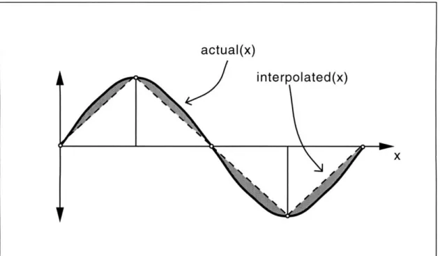
Rather than duplicate these results, a different approach is taken here. At a very basic level, it will attempt to quantify the error incurred by different interpolation methods in the spatial domain in a way that is appropriate to the image warping application. To facilitate analysis, this will be done in one dimension. First, take a continuous sinusoid of frequency

f Hz, actual (t) = sin (27tft). Next, sample this wave at 1/T Hz to produce,

samples [n] = sin( 274). Finally, using these samples and the selected interpolation

method, reconstruct the continuous sinewave. The reconstruction error is then calculated as follows:

b

ReconstructionError lactual (t) - interpolated (t) Idt ReconstructionError =

J (b - a)

a

Reconstruction Error Calculation (4.1)

This can be interpreted graphically as the area between the two functions divided by the length over which the area is being computed. Figure 4.1 shows this graphical interpreta-tion.

Figure 4.1: Reconstruction error illustration.

The length of integration is taken to be one complete period of the sinewave. The reconstruction error is calculated and averaged for all possible phase shifts of the sample points relative to the sinewave to give the expected error. This gives the average vertical separation between the two functions, and because it is computed for all phase shifts, expected error is an appropriate name.

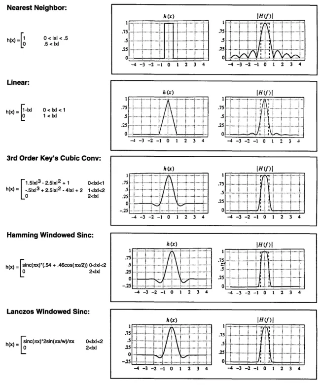
A few different interpolation kernels will be examined in this manner. Figure 4.2 shows these kernels and their frequency responses.

h (x) IH(f) l 1 ... ... .. o5 .75 75 ·. .5 .5 .25 .25 -4 -3 -2 -1 0 1 2 3 4 -4 -3 -2 -1 0 1 2 3 4 Linear: h(x) = -xl 0 < IxI < 1 01 1 < lxli

3rd Order Key's Cubic Conv:

1 .5 1x l3

-2.51x12 + 1 0<Ixl<l

h(x) = -.51x 3 + 2.51x12 - 41x1 + 2 1<1x1<2

L0 2<lxl

Hamming Windowed Sinc:

h(x) = inc(x) = nc)*(.54 + .46cos(nx/2)) 0<1xI<2

L

Lanczos Windowed Sinc:

h(x) = 0inc(nx )*2sin (irx/w)/x 0<IxI<2 2<Ixl h (x) IH(f) .75 ... i ... ... . ... . .5 ... ... ... .... .... ... ... .5S .25 -4 -3 -2 -1 0 1 2 3 4 -4 -3 -2 -1 0 1 2 3 4 h(x) IH(f)I -4 -3 -2 -1 0 1 2 3 4 I .1

I

1

Figure 4.2: Interpolation kernels and their frequency responses. Nearest Neighbor:

h(x) ₌

1

0< lxi <.5

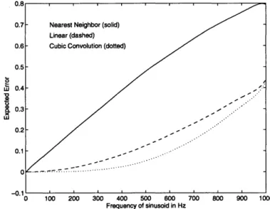
For each interpolation method, given a fixed sampling frequency of 1/T, a plot of expected error as a function of frequency of the underlying sinusoid is generated. This data is presented graphically in Figure 4.3 and Figure 4.4.

0.8

0.7- Nearest Neighbor (solid) Linear (dashed)

0.6- Cubic Convolution (dotted)

0.5 ,L 0.4 S0.3 0.2 0.1 0-0 :7 --. ---0.1 0 100 200 300 400 500 600 700 800 900 1000 Frequency of sinusoid in Hz

Figure 4.3: Expected error vs. frequency for sampling rate of 2000Hz.

Figure 4.3 shows the expected error for three basic interpolation methods. These are nearest neighbor interpolation, linear interpolation, and third order cubic convolution. The sampling rate is fixed at 2000Hz in this experiment. The horizontal axis is the frequency of the underlying sinusoid. It ranges from 0 to 1000Hz. If the frequency is allowed to go beyond 1000Hz, then the signal is no longer Nyquist sampled and the expected error value will include the affects of aliasing, which is not meant to be measured. The vertical axis is the expected error, as defined in Equation 4.1.

As expected, nearest neighbor interpolation is the poorest performer. Linear interpola-tion is the next best, followed by cubic convoluinterpola-tion interpolainterpola-tion. There is a marked dif-ference between all three methods. This is directly linked to the fact that nearest neighbor uses one sample point for interpolation, and linear and cubic use two and four sample

points, respectively. This basic result is also confirmed by frequency domain interpreta-tion. 0 Lil In Frequency of sinusoid in Hz

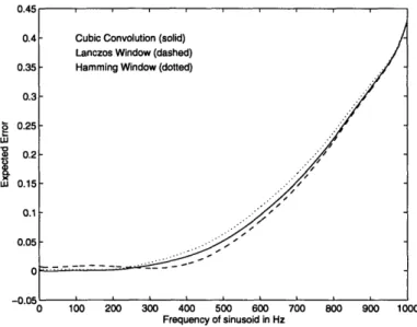
Figure 4.4: Expected error vs. frequency for sampling rate of 2000Hz.

Figure 4.4 shows expected error for two other interpolation methods. Cubic convolu-tion is included as a reference to Figure 4.3. The Lanczos windowed sinc kernel is the best performer for the higher frequencies, but cubic convolution is better at lower frequencies. Overall though, their performance is very similar because they all use four sample points. In hardware, if the interpolation kernel values are precalculated, then all methods that use a four-by-four interpolation kernel should produce nearly identical results, given a fixed sampling rate.

In the preceding calculations of expected error, the sampling rate was fixed, and the expected error was found as a function of frequency of the underlying sinusoid. An equiv-alent analysis could be made by fixing the frequency of the sinusoid and varying the sam-pling rate, since the expected error will be the same for two sets of samsam-pling rates and frequencies, (sample_rate_l, frequency_l) and (sample_rate_2, frequency_2) if freq_1/

sample_j = freq_2/sample_2. For example, using the same interpolation method, the

expected error would be identical for a 200Hz sinusoid sampled at 1000Hz as for a 400Hz sinusoid sampled at 2000Hz.

4.3 Sampling Rate Issues

An interesting question then develops. Could an otherwise poor interpolation method give superior results if we oversample the analog signal. For example, could linear inter-polation with an oversampled signal give less error than cubic convolution interinter-polation with a Nyquist sampled signal? The answer is clearly, yes. But, how much oversampling is needed? The following analysis will attempt to quantify these things through analysis in the time domain.

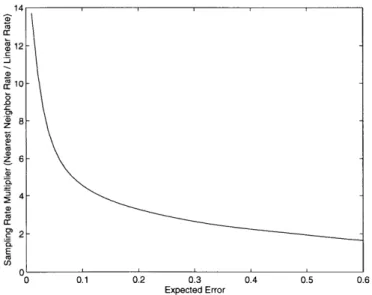
Figure 4.5 shows the "sampling rate multiplier" for linear interpolation versus cubic convolution interpolation as a function of the expected error. This multiplier is defined as follows. If we sample a sinusoid of a given frequency, the expected error under a cubic convolution interpolation scheme is the same as the expected error using a linear interpo-lation scheme when the sampling rate for the linear scheme exceeds that of the cubic scheme by the sampling rate multiplier for that particular expected error. If a large expected error is tolerable, then the sampling rate multiplier is quite small. However, as the desired expected error approaches zero, the multiplier grows rapidly.

6 Expected Error

Figure 4.5: Sampling rate multiplier (linear vs. cubic convolution).

Figure 4.6 shows the same sort of information, except here the vertical axis is the sam-pling rate multiplier for nearest neighbor interpolation versus linear interpolation.

0 0.1 0.2 0.3

Expected Error 0.4 0.5 0.6

Figure 4.6: Sampling rate multiplier (nearest neighbor vs. linear).

It has the same basic shape as Figure 4.5 except that the multiplier is considerably larger for any given expected error. This is because nearest neighbor interpolation is such a poor overall performer. Because the multiplier is so large and results at least as good as linear interpolation on a Nyquist sampled image are desired, this case will not be analyzed further.

There are many interesting implications that develop from Figure 4.5. Specifically, note that for a tolerable error of .02, doubling the sampling rate and using a linear interpo-lation scheme is comparable to cubic convolution. This leads to many interesting possibil-ities for an efficient hardware implementation. Instead of performing a two-dimensional third-order cubic convolution interpolation for resampling on a Nyquist sampled image, it might be possible to perform two-dimensional linear interpolation (commonly referred to as bilinear interpolation) for resampling on a double density sampled image. The interpo-lation kernel size would be decreased from 4x4 to 2x2. This leads to a reduction in the cost and number of components needed. The penalty in this approach is incurred in increasing the sampling rate by a factor of two. There are two approaches to this. First, the analog image could be sampled at twice the previous rate. The prohibitive disadvantage of this approach is that the warper can no longer be a modular part of a complete vision system, since it requires a different digitizer and image size for input. The second approach, which is the one that will be examined, is to include a digital upsampler in the warper. This takes the Nyquist sampled digital image and upsamples it by a factor of two in both directions. Then this image is warped, using bilinear interpolation for resampling. This is a specific example of a more general approach to performing high quality image warping efficiently in hardware. The general approach is to upsample using a good filter, next warp using a lower quality filter, finally downsample to give the final image. This approach will be examined in detail.

Chapter

5

High Quality, Efficient Image Warping

5.1 General Description of Method.

As discussed in previous chapters, there are two components to an image warp: spatial transformation and resampling through interpolation. In the interpolation step, an area of pixels around the referenced input location is used to compute the output pixel value. The larger the number of pixels used, the more accurate the resampling can be. However, as the number of pixels used increases, so does the cost and complexity of the hardware implementation. The method described in this chapter deals primarily with a way to improve the accuracy of the resampling without a drastic increase in complexity.

One standard approach to performing the interpolation required for the resampling uses a 2x2 neighborhood of pixels around the referenced address in the source image to calculate each output pixel value. This is commonly called bilinear interpolation, which simply refers to linear interpolation in two dimensions. Chapter 6 describes such a hard-ware design in detail. For a real-time implementation with reasonable clock rates, this means that every clock cycle, four pixels values must be accessed simultaneously. These pixel values are then multiplied by the appropriate weights and summed to give the output pixel value. In hardware, this corresponds to four separate memory banks that can be accessed in parallel. Also, the four weighting coefficients must be generated, based on the sub-pixel location of the reference point. Finally, a four-term sum of products must be per-formed. The difficulty with this model comes when bilinear interpolation is no longer ade-quate. In applications that require repeated warping of the same image, or even just high quality sub-pixel translations, bilinear interpolation gives poor results. The next highest quality interpolator uses a 3x3 pixel area in the source image to compute each output pixel

value. If the same paradigm is used, it leads to an unwieldy implementation. Now, nine separate memory banks, nine coefficients, and a nine-term sum of products are required. In applications where size, power and cost are at a premium, this is an unacceptable solu-tion. If an even better interpolation is required, for example 4x4 or 6x6, the problem is even worse. There are some optimizations that can be made under this approach, but the fundamental problem of quadratic growth will always exist. One common approach to avoiding this problem is the use of a two-pass method. This approach works well in many specialized cases. It cannot, however, accommodate a general flow-field warp without costly computation overhead.

The following provides a high level description of a method for performing an arbi-trary image warp that can achieve high-quality interpolation while bypassing some of the limitations described above. The basic system is shown in Figure 5.1.

Figure 5.1: High quality warp system.

The three basic steps are to first increase the sampling rate, then warp the image using a lower quality interpolator for resampling, and finally downsample the image to its origi-nal size. These steps and their implementation are described below.

Typical digital images to be warped are sampled at the Nyquist rate. The first step in the new warping method is to increase the sampling rate above this point. This can be done by either sampling the analog image at a higher rate or by digitally processing an

already Nyquist-sampled image to increase its sampling rate. The latter of these two approaches will be taken to maintain the modularity of the warper within a larger image processing system.

Because the input image to the system is sampled at or above the Nyquist rate, it is a complete representation of the underlying analog image. Therefore, theoretically, it is pos-sible to obtain the exact value of that analog image at any point, even though only the sampled points are available. To achieve an efficient implementation, we limit the oper-ation to an upsampling by a factor of 2N , where N is a positive integer. This upsampling is done in both the vertical and horizontal directions. For example, if the input image is 512x512 pixels, upsampling by a factor of 2 would give an image of size 1024x1024. Upsampling by a factor of 4 would give a resulting image size of 2048x2048. It is impor-tant to use a very high quality interpolation method to obtain the values of the upsampled image.

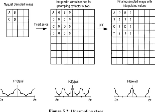
Conceptually, the upsampling occurs in two steps. The first step is to insert the appro-priate number of zeros into the image. For example, if the image is being upsampled by 2, then every other value in the upsampled image is zero. The values at the other locations are the original samples from the source image. Then this intermediate image is lowpass filtered to give the final upsampled image. The original image is critically sampled. Insert-ing zeros compresses the Fourier transform by a factor of two. The final lowpass filter leaves only a single copy of the compressed transform centered around every integer mul-tiple of 27c. The spatial and corresponding frequency domain interpretation of this process are shown in Figure 5.2.

Nyquist Sampled Image

Insert zeros

Image with zeros inserted for upsampling by factor of two

A 0 C 0 0 0 0 0 0 0 0 0 LPF B 0

Final upsampled image with interpolated values A ? B ? C ? D ? ? ? ?7 ? IH1(ejm)l

-2s

21L

Figure 5.2: Upsampling stage.

At this point, it is clear why a high quality lowpass filter is needed for the interpola-tion. This lowpass filter must cleanly eliminate the undesired frequency components while leaving the desired frequency components relatively undisturbed.

This sort of constrained upsampling can be performed quite efficiently in hardware. The Pyramid Chip, developed at the David Sarnoff Research Center, is an excellent exam-ple of how this operation may be performed [12]. The upsampling can be imexam-plemented as a separable operation, which maps well to hardware. For the warping application, it is expected that a higher quality filter than the Pyramid Chip can provide will be needed. Still, a 4-tap or 6-tap fixed coefficient filter to perform the upsampling can be implemented in an field programmable gate array fairly easily.

IH3(eju)l

.×.

A./,

In summary, there are two variables to consider in the upsampling procedure. The first is the amount by which the image will be upsampled. We constrain these values to be 2, 4, 8, etc. The second is the quality of the lowpass filter employed to perform the interpola-tion. It is expected that a 4-tap or 6-tap filter will be adequate. However, implementing a filter with more taps does not lead to a huge increase of complexity. The desired quality of the resultant warped image will determine appropriate values for these two variables.

Step two in the procedure is to warp this oversampled image using a lower quality interpolation filter for resampling. Because the image has been upsampled, its frequency content has been compressed. A lower quality filter used in the resampling step for the warp can give good results, as long as it has good characteristics over this smaller region of the frequency spectrum. This is shown in Figure 5.3.

Frequency Domain Interpretation

Original Digital Image

Poor LPF

no downsampling needed

Final Image

Upsampled Image

LJ

I

Poor

LPF

downsam

for Resampling

rirv

Figure

5.3:

Figure 5.3: Frequency domain comparison.

49

Final Image

Overall, the warp using the upsampled image does a better job of eliminating the unwanted duplicate high frequencies while leaving the desired frequencies undisturbed. Using a lower quality filter at this warping stage can drastically reduce the complexity, as it will use a smaller neighborhood of pixels.

Finally, the warped image is downsampled to the size it was before the upsampling occurred. In practice, this can be performed quite efficiently by modifying the geometric transformation function. The downsampling is then inherent in the warp equation. This approach combines steps two and three into one process.

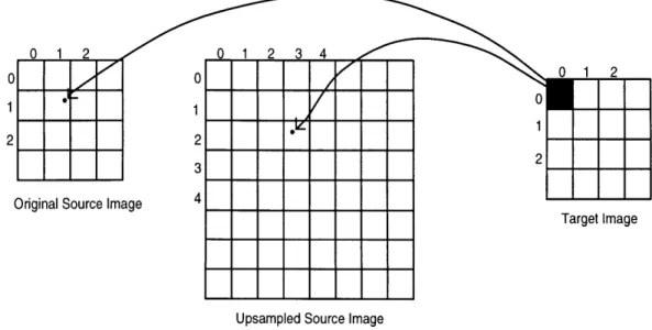
Figure 5.4 shows how the downsampling is performed as part of the image warp.

Upsampled Source Image

Figure 5.4: Downsampling as part of image warp.

In this example, the standard geometric transformation specifies that the value in the target image at [0,0] should come from the source image location (xl = 1.7, yl = 1.2). This value at a nonintegral location would be determined by looking at a neighborhood of pixels around this location. To access the same point in the upsampled image, simply

mul-tiply the referenced address by 2. In this case, the address to reference in the upsampled source image would be (x2 = 3.4, y2 = 2.4). If the image was upsampled by a factor of 4, the referenced address would be multiplied by 4. Then a neighborhood of pixels around this address is used to determine the output value. Besides this modification, the warp is performed identically to the standard method described earlier. In effect, the neighborhood of pixels that is used in the upsampled image corresponds to sample points of the original analog image that are closer to the desired location than an equal-sized neighborhood of pixels in the original Nyquist sampled image.

At first glance, one drawback to this approach for a hardware implementation seems to be that the warp will require more time to complete. The upsampling stage increases the size of the image. This data then needs to be passed to the warper memory, where it can be accessed at random. If the image data comes to the upsampling stage at a rate of one pixel per clock cycle and leaves the upsampling stage to be stored in the memory for the warp at the same rate, then there is a backlog delay incurred in this process, because more pixels are leaving the upsampling stage than are coming in.

However, this problem can be avoided. Basically, all that is required is to increase the bandwidth leaving the upsampling stage relative to the bandwidth entering the upsampling stage by the same factor as the increase in image size. There are many possible ways to do this. For example, assume that the warping stage uses bilinear interpolation. Then, there are four separate memory banks holding the image to be warped. If the upsampling stage upsamples by a factor of two in both directions, then the required bandwidth leaving the upsampling stage is four times that of the bandwidth entering it. So, if the image is enter-ing the upsamplenter-ing stage at one pixel per clock cycle, it should leave at four pixels per clock cycle. Because there are four independent memory banks holding the image, it is

possible to write four pixels to this memory each clock cycle, thus meeting the bandwidth requirements. Then the only delay incurred will be a minor pipeline delay.

In conclusion, this approach to image warping gives a number of advantages (particu-larly for a hardware implementation) over the standard one-pass approach. It provides:

1. A method of image warping that doesn't grow quadratically in complexity with the resampling accuracy. The complete warping process is implemented in two steps. The first is upsampling. The second is warping with downsampling. These two steps can be tuned together to produce the desired quality warp. The complexity of the second step can be fixed at a reasonable setting. Then the upsampling step can be changed to give the desired quality.

2. A modular, independent, warping function that can process arbitrary spatial trans-formations. There are many specialized warping algorithms that achieve excellent results for particular applications; for example, rotation [11]. The warping procedure described in this thesis takes a Nyquist sampled image as input and produces a warped image as output. The warp function is not constrained to a particular type; it can be an arbitrary flow field.

3. A method of upsampling that is well suited for hardware implementation. The upsampling is constrained to a factor of 2N, and is implemented using a separable filter. Both these factors lead to an efficient hardware implementation.

4. A method of downsampling that is simple to implement within the warping struc-ture. Because the image was upsampled by a factor of 2N, the downsampling can be per-formed as part of the warp by multiplying the vertical and horizontal components of the referenced source address by this factor. This multiplication is simply a bit shift. This

5.2 Comparison with Standard Techniques

Section 5.1 described the proposed approach to warping in a very general sense. Now, we examine the performance of the method for some very specific cases. There are basically three degrees of freedom in the general method. These are: the amount by which the orig-inal image is upsampled, the interpolation method used for upsampling, and forig-inally, the interpolation method used for warping. In determining these factors, it must be kept in mind that the final goal is an efficient method for real-time image warping in hardware. Therefore, in the following analysis two of these factors will be fixed. First, the original image will always be upsampled by a factor of two in the vertical and horizontal direc-tions. Second, the interpolation method in the warping stage will be fixed at bilinear. There are a number of advantages to doing this. Upsampling by a non-integer factor adds unnecessary complexity to the hardware. And, upsampling by a factor of two (as opposed to larger factors) can be implemented in hardware very efficiently. If the warping stage uses bilinear interpolation, a 2x2 pixel neighborhood is used. As discussed earlier, for a real-time hardware implementation, this leads to four separate memory banks, four weighting coefficients, and a four-term sum of products. Better interpolation methods for the warping stage would required an increase in all these quantities. Finally, if the image is upsampled by a factor of two, and if the warping stage has four separate memory banks that can be accessed in parallel, then it is possible to pipe the image data through the upsampling stage and into the warp memory without a backlog of the data in the upsam-pling stage. Under these constraints, the only variable left to manipulate is the upsamupsam-pling method. The proposed method of image warping under different upsampling methods will then be compared with other common approaches.

The familiar Lena image will be used for all of the tests. Two measures will be used to assess the quality of the warp. The first will be a measure of Root Mean Square (RMS)

error between the final warped image and the original image. The second will be a visual comparison. A total of five methods will be examined here. These are listed in Table 5.1.

Name Description

Bilinear No upsampling.

Bilinear interpolation used in warp.

(2x2 pixel area.)

Keys-3 No upsampling.

Third order cubic convolu-tion (a=-.5) used in warp. (4x4 pixel area).

Keys-4 No upsampling.

Fourth Order Cubic Con-volution used in warp. (6x6 Pixel Area). Up2(Keys-3) Upsample by two using

Keys-3.

(4 tap separable)

Bilinear interpolation used in warp.

(2x2 pixel area).

Up2(Keys-4) Upsample by two using Keys-4.

(6 tap separable)

Bilinear interpolation used in warp.

Table 5.1: Warping Method Descriptions

The first test will be image rotation. The Lena image is rotated by 22.5 degrees a total of 16 times to bring it back to its original orientation. Then, the RMS error between this image and the original is taken. The results are summarized in Table 5.2.