HAL Id: hal-01130187
https://hal.sorbonne-universite.fr/hal-01130187
Submitted on 11 Mar 2015
HAL is a multi-disciplinary open access
archive for the deposit and dissemination of
sci-entific research documents, whether they are
pub-lished or not. The documents may come from
teaching and research institutions in France or
abroad, or from public or private research centers.
L’archive ouverte pluridisciplinaire HAL, est
destinée au dépôt et à la diffusion de documents
scientifiques de niveau recherche, publiés ou non,
émanant des établissements d’enseignement et de
recherche français ou étrangers, des laboratoires
publics ou privés.
A cautionary note on the use of EESC-based regression
analysis for ozone trend studies
Jayanarayanan Kuttippurath, G. E. Bodeker, H. K. Roscoe, Prijitha J. Nair
To cite this version:
Jayanarayanan Kuttippurath, G. E. Bodeker, H. K. Roscoe, Prijitha J. Nair. A cautionary note on
the use of EESC-based regression analysis for ozone trend studies. Geophysical Research Letters,
American Geophysical Union, 2015, 42 (1), pp.162-168. �10.1002/2014GL062142�. �hal-01130187�
RESEARCH LETTER
10.1002/2014GL062142 Key Points:• Presents a thorough analysis on the EESC-based regression
• The EESC-based regression is inappropriate for estimating ozone trends
• Recommends a reinterpretation of the previous EESC-based trend estimates Correspondence to: J. Kuttippurath, [email protected] Citation: Kuttippurath, J., G. E. Bodeker, H. K. Roscoe, and P. J. Nair (2015), A cautionary note on the use of EESC-based regression analysis for ozone trend studies, Geophys. Res.
Lett., 42, 162–168,
doi:10.1002/2014GL062142.
Received 6 OCT 2014 Accepted 11 DEC 2014
Accepted article online 15 DEC 2014 Published online 6 JAN 2015
A cautionary note on the use of EESC-based regression
analysis for ozone trend studies
J. Kuttippurath1, G. E. Bodeker2, H. K. Roscoe3, and P. J. Nair4
1CNRS/LATMOS, UPMC University of Paris 06, Paris, France,2Bodeker Scientific, Alexandra, Central Otago, New Zealand, 3British Antarctic Survey, Cambridge, UK,4Centre for Earth Science Studies, Thiruvananthapuram, India
Abstract
Equivalent effective stratospheric chlorine (EESC) construct of ozone regression models attributes ozone changes to EESC changes using a single value of the sensitivity of ozone to EESC over the whole period. Using space-based total column ozone (TCO) measurements, and a synthetic TCO time series constructed such that EESC does not fall below its late 1990s maximum, we demonstrate that the EESC-based estimates of ozone changes in the polar regions (70–90◦) after 2000 may, falsely, suggest an EESC-driven increase in ozone over this period. An EESC-based regression of our synthetic “failed Montreal Protocol with constant EESC” time series suggests a positive TCO trend that is statistically significantly different from zero over 2001–2012 when, in fact, no recovery has taken place. Our analysis demonstrates that caution needs to be exercised when using explanatory variables, with a single fit coefficient, fitted to the entire data record, to interpret changes in only part of the record.1. Introduction
Emissions of anthropogenic ozone depleting substances (ODSs), and their steep increase from the early 1970s to the end of the twentieth century, caused severe ozone loss in stratosphere and in particular over polar latitudes [World Meteorological Organization (WMO), 2007]. As a result of the Montreal Protocol and its amendments and adjustments, ODS emissions have now declined significantly [World Meteorological
Organization (WMO), 2011]. Although the resultant halogen loading of the polar stratosphere has declined
slowly since the turn of the century [e.g., Froidevaux et al., 2006], it is not yet clear whether the springtime ozone loss inside the polar vortices is responding to that decline [WMO, 2011]. While previous studies have reported positive trends in middle- and high-latitude ozone since ∼2000 [Nair et al., 2013; Kuttippurath et al., 2013; Salby et al., 2011], these increases cannot be unambiguously regarded as the second stage of ozone recovery, i.e., the occurrence of statistically significant increases in ozone above previous minimum values due to declining EESC [WMO, 2007].
Many methods have been employed to quantify trends in ozone, with the equivalent effective stratospheric chlorine (EESC) [e.g., Wohltmann et al., 2007; Stolarski et al., 2006] and piecewise linear trend (PWLT) [e.g., Reinsel et al., 2002; Nair et al., 2013] methods being the most widely used. The first correlates ozone against EESC [Stolarski et al., 2006], while the second quantifies the trend over the full period as well as the change in the trend after some prescribed breakpoint [Reinsel et al., 2002]. Both methods usually include additional basis functions in the regression model to account for other drivers of changes in ozone, e.g., atmospheric circulation represented by poleward heat flux and the quasi-biennial oscillation (QBO) in equatorial stratospheric winds that modulates poleward planetary wave propagation. The goal of this study is to demonstrate that fitting EESC to describe changes in high-latitude TCO from 1979 to 2012, and then interpreting the single fit coefficient as a description of the ozone change from 2000 to 2012, can suggest a recovery in polar ozone from the effect of ODSs when, in fact, no such recovery has taken place.
Space-based TCO measurements from 1979 to 2012 are first used to analyze ozone changes over the polar regions (70–90◦). The estimated trends are compared to published results in section 3.1 to check the robustness of the regression procedure. Then, in section 3.2, the EESC and PWLT regression models are applied to interpret long-term changes in ozone from a synthetic TCO time series that is constructed to mimic what ozone may have looked like under a failed Montreal Protocol, i.e., where EESC remains at its maximum level from the late 1990s to 2012. The resulting analysis is discussed in section 4 with a focus on the appropriateness of the EESC and PWLT regression models to describe changes in ozone since 2000.
Geophysical Research Letters
10.1002/2014GL062142
Figure 1. (top) The temporal evolution of equivalent effective
stratospheric chlorine (EESC, corresponds to the WMO A1-2010 scenario) in pptv in an inverted vertical scale. The horizontal line indicates 4000 pptv. The principle of trend estimation using the piecewise linear trend (PWLT) is also demonstrated. See text (section 2) for discussion of the slope termsm1andm2. (bottom) TCO averaged over the latitude bands 70–90◦used for the regression analysis in this study for the Arctic winter (average of December, January, and February (DJF)) and Antarctic spring (average of September, October, and November (SON)).
2. Data and Methods
A consolidated TCO data set constructed from multiplesatellite-based instruments, corrected for instrumental biases through validation with ground-based measurements, has been used as the basis analyzing secular changes in ozone from 1979 to 2012. This data set is an update of that published in Müller
et al. [2008] and is available at http://
www.bodekerscientific.com/data/ total-column-ozone/. This data set is well suited for trend analyses and has a clear advantage over individual ozone data records (e.g., as demonstrated in
Nair et al. [2013]). While the ozone data
used for the annual mean (ANN) trend analysis includes all 34 years of data, the Antarctic spring analysis considers data from September 1979 to October 2011. Figure 1 (bottom) shows the evolution of Arctic winter (December, January, and February (DJF)) and Antarctic spring (September, October, and November (SON)) TCO, the periods when ozone loss maximizes in those regions, which is then used for later analysis.
The regression model incorporates explanatory time series for all processes known to influence the long-term evolution of ozone, which include the following: (a) the wave-driven Brewer-Dobson circulation, represented by the heat flux at 100 hPa, calculated from the European Centre for Medium-Range Weather Forecasts Reanalysis (ERA)-Interim meteorological reanalyses, averaged over 45◦–75◦N/S [Kuttippurath and
Nikulin, 2012]. This represents the wave momentum entering the stratosphere from the troposphere. (b)
The Antarctic Oscillation (AAO) and El Ni ˜no–Southern Oscillation (ENSO) to consider the changes in TCO driven by local meteorological patterns. (c) The solar flux at 10.7 cm wavelength. (d) Zonal mean zonal winds at 30 and 10 hPa to account for the latitudinal and vertical difference in the influence of the QBO on the atmospheric circulation. (e) Volcanic aerosol loading to account for contributions from the El Chichón (1982) and Mount Pinatubo (1991) volcanic eruptions that contributed to heterogeneous ozone loss.
The EESC time series used for the analysis (Figure 1 (top) using an inverted vertical scale) corresponds to the WMO A1-2010 scenario with a mean age of air of 5.5 years for the polar stratosphere, an age of air spectrum width of 2.75 years, and a bromine scaling factor of 60 to account for the greater ozone depleting potential of bromine on a per atom basis over chlorine [Newman et al., 2007]. This is just one scenario that could influence recent ozone trends, an alternative might be that a higher age of air could delay ozone recovery. The TCO change in the EESC-based regression analysis is statistically modeled as
O3(t) = K + C1EESC(t) + C2Aerosol(t) + C3HeatFlux(t) + C4SolarFlux(t) + C5ENSO(t)
+ C6QBO 10 hPa(t) + C7QBO 30 hPa(t) +𝜖(t) (1) where t is the decimal year, K is a constant,𝜖 is the residual, and C1to C7are the regression model
coefficients of the respective proxies. In the PWLT regression, the C1EESC(t) term is replaced by (C1t1+ C2t2)
in the above equation, where C1is the linear trend and C2is the change in trend after the selected
turnaround year, t1is the number of years from 1979 to 2012, and t2is the number of years from 2001 (the
turnaround year) to 2012 and set to zero prior to 2001. The turnaround year is set as 2001 congruent with the year when EESC maximizes in the polar regions, as shown in Figure 1. The regression analysis for the Antarctic TCO data is performed by the method described in Kuttippurath et al. [2013]. The trend in EESC can be expressed in ppt/yr and, in this way, converted to an equivalent TCO trend in Dobson unit (DU)/yr by
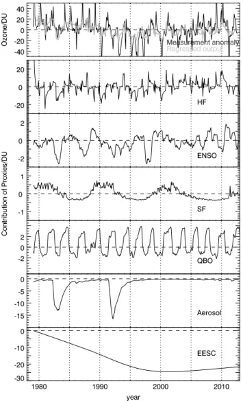
Figure 2. The regression results based on the annually averaged TCO
data in the Arctic (70–90◦N). (top to bottom) The contribution from heat flux (HF), El Ni ˜no–Southern Oscillation (ENSO), solar flux (SF), quasi-biennial Oscillation (QBO), Aerosol, and equivalent effective stratospheric chlorine (EESC).
multiplying the EESC trend by the regression coefficient (C1) which
has units of DU/ppt [Stolarski et al., 2006]. Trends derived from the PWLT regression are in DU/yr [Reinsel et
al., 2002]. The uncertainty on the
regression model fit coefficients is determined using the generalized least squares method and by considering the autocorrelation of residuals with 1 year lag [Press et al., 1989].
3. Results and Discussions
3.1. Trend Analysis: Observed Time Series
The regression model described above has been applied to monthly mean Arctic and Antarctic TCO data using both the PWLT and EESC constructs of the regression model to estimate the contribution of various proxies to the TCO change. The EESC-based analysis for the Arctic winter is shown in Figure 2. Both the measurements and regression fit exhibit a clear decline in TCO from the beginning of the record until the EESC peaks around 2001. The ozone losses directly following the volcanic eruptions in 1982–1984 and 1992–1994 are also significant, with maximum contributions of about −16 DU in 1983 and −19 DU in 1992. Solar activity influences TCO by about 0.5–0.8 DU from solar minimum to maximum, in agreement with previous studies [Hood and Zhou, 1998;
Soukharev and Hood, 2006]. The
contribution of planetary wave-driven ozone transport is important in the Arctic, as the winters are prone to frequent sudden stratospheric warmings (SSWs) which affect the stability of the vortex and ozone loss in each spring [e.g., Kuttippurath and Nikulin, 2012]. Winters with strong wave activity, and concomitant warmer temperatures, show elevated ozone, e.g., +20 DU in 1979 and +15 DU in 2010, years in which major SSWs occurred. Suppressed wave activity results in a strong vortex and so colder temperatures, which suppresses ozone, e.g., −15 to −18 DU in 1981, 1983, 1990, and 2000. The QBO and ENSO also modulate polar ozone, each by about 2 DU peak to peak. In the Antarctic the contribution of each explanatory variable to the total signal is similar to that for the Arctic though the amplitudes differ.
Table 1 shows the PWLT- and EESC-based ozone trends for the periods 1979–2001 and 2001–2012 for the annual mean (ANN) and for the ozone loss peak periods, i.e., DJF for the Arctic and SON for the Antarctic (shown in Figure 1). The trends in annual mean TCO over the Arctic are statistically significantly different from zero at the 95% level for both periods and using both methods. The larger uncertainties for PWLT trends from 2001 to 2012 are consistent with the small number of years in that period, which could then alias with slower cycles such as the solar cycle. This differentiation in uncertainty between the short latter period and long earlier period is not possible when regressing against EESC which considers all years together. The estimated trends are in agreement with those computed by Kiesewetter et al. [2010] who
Geophysical Research Letters
10.1002/2014GL062142
Table 1. The Annual and Seasonal TCO (Both Measurements and Synthetic
Data) Trends in DU/yr (Dobson Unit Per Year) With 95% Confidence Intervals (Given as the Error Bars of Trend Values) Estimated Using Both Piecewise Linear Trend (PWLT) and Equivalent Effective Stratospheric Chlorine (EESC) Regression Analyses for the 1979–2001 (Pre-EESC Maximum) and 2001–2012 (Post-EESC Maximum) Periodsa
1979–2001 Method Arctic Antarctic Synthetic ANN EESC −1.12 ±0.53 −1.77 ±0.56 −1.09 ±0.25
PWLT −1.34 ±0.57 −2.00 ±0.63 −1.16 ±0.28 Winter or Spring EESC −1.66 ±1.48 −3.65 ±0.69 −1.05 ±0.10 PWLT −2.24 ±1.24 −4.20 ±0.90 −1.16 ±0.19 2001–2012
ANN EESC +0.25 ±0.12 +0.40 ±0.13 +0.25 ±0.06 PWLT +1.92 ±1.21 +1.58 ±1.35 +0.59 ±0.59 Winter or Spring EESC +0.39 ±0.35 +0.94 ±0.18 +0.25 ±0.02 PWLT +4.09 ±2.56 +3.58 ±2.33 +0.41 ±0.39
aThe satellite data are averaged over the latitude bands of 70–90◦N for Arctic
and 70–90◦S for Antarctic. The annual trend estimates are represented by ANN, and the seasonal trend estimates are represented by winter or spring (winter or DJF for Arctic and Synthetic and spring or SON for Antarctic). The Antarctic trends are over the period 1979–2011, instead of 1979–2012 in other cases. The trend from EESC-based regression is in ppt/yr, and the regression coefficient of EESC from the regression is in DU/ppt; hence, the trend in ozone is in DU/yr. Trends from PWLT regressions are inherently in DU/yr. Note also that the PWLT- and EESC-based trend values are not directly comparable and are given together here for discussion only.
found the largest trends of −1.3 to −1.6 ± 0.9 DU/yr (∼ 0.5 ± 0.35%/yr) in the Arctic winter and spring over 1979–1999 using a similar method. Our PWLT trend values are also comparable to those of Wohltmann
et al. [2007], who estimate about −1.2 ± 0.4 DU/yr in March for 1979–2003. A similar trend was also found
in a satellite ozone data set over 1979–2004 by Brunner et al. [2006], for which equivalent latitude and potential temperature coordinates were applied to delineate trends in different dynamical regimes. The small differences among the results derived from the various studies are within their stated uncertainties. In the Antarctic, the regression analysis estimates trends of about −1.7 to −2 ± 0.6 DU/yr in the annual mean from 1979 to 2001 by both methods and about +0.4 ± 0.13 DU/yr for the EESC-based regression and +1.6 ± 1.4 DU/yr for the PWLT regression in the annual mean for 2001–2012. In SON the estimated trends, using both methods, in both periods, are statistically significantly different from zero at the 95% level. These estimates are in very good agreement with those computed from ground-based and space-based data in the Antarctic vortex, i.e., around −4.5 ± 0.8 DU/yr over 1979–2000 and about +2.8 ± 2.7 DU/yr from the PWLT-based regression over 2000–2010 as reported in Kuttippurath et al. [2013]. The trends are also in good agreement with those found by Yang et al. [2008], who derived −4.9 ± 1.5 DU/yr over 1979–1996 from ground-based and satellite data inside the vortex for September. A similar trend of around −4 DU/yr was also deduced from a satellite-based ozone data set by Brunner et al. [2006] over 1979–2004. The EESC-based trends are consistent with those derived from chemistry climate model simulations for 1997–2009, which show an EESC-based trend of about +1 DU/yr [Austin et al., 2010; Kiesewetter et al., 2010]. Our EESC-based result is in agreement with the analysis presented by Salby et al. [2011], although they do not provide any trend values but only state that the trends are significant at the 99.5% confidence interval. The studies cited above report trends over different time periods which may account for the small differences in trend values in addition to those resulting from different input data and analysis methods.
3.2. Trend Analysis: Synthetic Data With Failed Montreal Protocol With Constant EESC
Since we have already analyzed the robustness of the regression models through comparisons to other published results, we now assess the principle and usefulness of the EESC-based regression for finding and interpreting ozone trends. As a basis for this analysis we have constructed a synthetic data set by
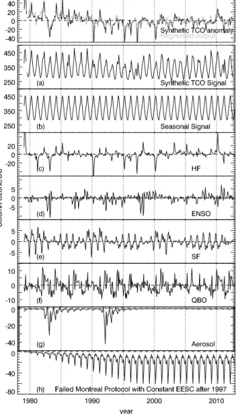
Figure 3. (a) The synthetic TCO data used for testing the regression
methods. The TCO anomaly made from the synthetic time series and its regressed output based on the EESC regression model (top figure), and (b–h) the panels below show input data choice for making the TCO signal.
combining contributions from multiple basis functions but where EESC follows a failed Montreal Protocol, i.e., there is no decrease in EESC after 1996; EESC remains at its peak value after 1996. Figure 3 shows the seven constituent time series for the synthetic TCO signal as well as the regression model fit to the resultant anomalies. We have applied the same regression models used above (section 3.1) to determine trends in the synthetic time series. The resulting trend estimates (for ANN and DJF) using the EESC-based and PWLT regressions are listed in Table 1 (right). This synthetic data set is not specifically for the Antarctic or Arctic,
and therefore, only one set of results is shown. While the 2001–2012 EESC-based trend is statistically significantly different from zero at the 95% confidence interval, the PWLT-based trend is not for ANN. The key result here is that the EESC-based regression model estimates statistically significant positive
trends in ozone from 2001 to 2012 even though, by construction, the synthetic signal has constant elevated EESC over this period. Our trend analyses for midlatitudes yielded similar results (e.g., EESC-based trends of +0.40 ± 0.07 DU/yr
for ANN at 30–60◦N over
1997–2012) to confirm the findings for the polar latitudes. These demonstrate that the EESC-based regressions do not produce a reliable trend estimate over a subset of the data when the fit itself was performed over the whole time series. Therefore, a careful interpretation of the EESC-based results is warranted.
The cause of the failure of the EESC-based regression is by virtue of its design. Over the 22 year period from 1979 to 2001, EESC increased strongly and ozone decreased sharply, forcing a strong negative correlation between ozone and EESC, and thus, almost the same trend value as that derived from the PWLT-based regression is computed. In the ensuing 12 year period (2001–2012) there is only a small decrease in EESC and little increase in ozone (as the PWLT estimates confirm) which only slightly weakens the strong statistical anticorrelation driven by the 1979–2001 period. The single EESC fit coefficient, whose value is driven primarily by the ozone and EESC anticorrelation between 1979 and 2001, when used to quantify ozone trends from 2001 to 2012, produces statistically significant positive ozone trends for a time series constructed with a failed Montreal Protocol scenario. When it minimizes the sum of the squares of the residuals, the regression model gives more weight to the former period, since the variance is bigger there due to a comparatively longer period and more pronounced increasing EESC and decreasing ozone signals. This is by contrast to the PWLT method, which has two independent regression coefficients, and their
Geophysical Research Letters
10.1002/2014GL062142
multiple of time is the proxy, instead of EESC. Hence, trends estimated using the PWLT method are not vulnerable to the problems we identify above: they are caused by the fact of a single coefficient in the EESC method.
3.3. Trend Analysis: Arctic Ozone Recovery Signal?
The application of the PWLT-based regression model to the measured Arctic TCO for 2001–2012 shows a significant positive trend (Table 1). The PWLT-based Antarctic ozone trends are already discussed in
Kuttippurath et al. [2013], and this analysis confirms the significant trend in the post-EESC peak period
(2001–2012) for the SON season. However, statistically significant positive trends in Arctic TCO have not, to date, been reported. Our PWLT-based trend of +4 ± 2.6 DU/yr is comparable to that computed by
Kiesewetter et al. [2010] for the period 2000–2009, who simulated a trend of ∼ +3 DU/yr. However, their
trends were not statistically significant, perhaps because they did not include all relevant proxies in their analysis (e.g., heat flux). It is also possible that the additional 3 years of data available for our analysis pushes the results to be statistically significant. The number of years of data available, turnaround year, and the values at the end of a time series influence the derived trends and their statistical significance by the PWLT method. The 2001 to 2012 increase in Arctic TCO is apparent in the annual mean (+1.9 ± 1.2 DU/yr) and in winter/spring where peak ozone loss occurs every year. Although the EESC-based analyses cannot be used to unambiguously attribute these increases in ozone to decreases in EESC, the PWLT regressions show a positive trend in Arctic (70–90◦) ozone. However, analyses with different data sets are necessary to confirm this finding, and hence, a dedicated study on this topic will be presented in a separate article.
4. Conclusions
The utility of the EESC-based ozone trend estimation method has been investigated in the context of its ability to exclude a detection of polar ozone (70–90◦) recovery when a signal, absent of recovery, is used as input. The EESC-based regression fails this test and returns a trend over the 2001–2012 period that is statistically significantly different from zero at the 95% confidence level. This indicates that an EESC-based regression is inappropriate for unambiguously detecting ozone recovery from the effects of ODSs. The EESC-based trend estimation procedure, by its design, generates an ozone trend opposite in sign to the EESC trend over that period due to the anticorrelation between ozone and EESC. Our recommendation is not to use EESC-based regression for ozone trend estimation and suggest that previously published EESC-based ozone trend results may need to be reinterpreted in light of our findings.
References
Austin, J., et al. (2010), Decline and recovery of total column ozone using a multimodel time series analysis, J. Geophys. Res., 115, D00M10, doi:10.1029/2010JD013857.
Brunner, D., J. Staehelin, J. A. Maeder, I. Wohltmann, and G. E. Bodeker (2006), Variability and trends in total and vertically resolved stratospheric ozone based on the CATO ozone data set, Atmos. Chem. Phys., 6, 4985–5008, doi:10.5194/acp-6-4985-2006.
Froidevaux, L., et al. (2006), Temporal decrease in upper atmospheric chlorine, Geophys. Res. Lett., 33, L23812, doi:10.1029/2006GL027600. Hood, L. L., and S. Zhou (1998), Stratospheric effects of 27-day solar ultraviolet variations: An analysis of UARS MLS ozone and
temperature data, J. Geophys. Res., 103, 3629–3638.
Kiesewetter, G., B.-M. Sinnhuber, M. Weber, and J. P. Burrows (2010), Attribution of stratospheric ozone trends to chemistry and transport: A modelling study, Atmos. Chem. Phys., 10, 12,073–12,089, doi:10.5194/acp-10-12073-2010.
Kuttippurath, J., and G. Nikulin (2012), A comparative study of the major sudden stratospheric warmings in the Arctic winters 2003/2004–2009/2010, Atmos. Chem. Phys., 12, 8115–8129, doi:10.5194/acp-12-8115-2012.
Kuttippurath, J., F. Lefèvre, J.-P. Pommereau, H. K. Roscoe, F. Goutail, A. Pazmi ˜no, and J. D. Shanklin (2013), Antarctic ozone loss in 1979–2010: First sign of ozone recovery, Atmos. Chem. Phys., 13, 1625–1635, doi:10.5194/acp-13-1625-2013.
Müller, R., J.-U. Grooß, C. Lemmen, D. Heinze, M. Dameris, and G. E. Bodeker (2008), Simple measures of ozone depletion in the polar stratosphere, Atmos. Chem. Phys., 8, 251–264.
Nair, P. J., et al. (2013), Ozone trends derived from the total column and vertical profiles at a northern mid-latitude station, Atmos. Chem.
Phys., 13, 10,373–10,384, doi:10.5194/acp-13-10373-2013.
Newman, P., J. S. Daniel, D. Waugh, and E. R. Nash (2007), A new formulation of Equivalent Effective Stratospheric Chlorine (EESC), Atmos.
Chem. Phys., 7, 4537–4552, doi:10.5194/acp-7-4537-2007.
Press, W. H., B. P. Flannery, S. A. Teukolsky, and W. T. Vetterling (Eds.) (1989), Numerical Recipes, pp. 504–508, Cambridge Univ. Press, Cambridge, U. K.
Reinsel, G. C., E. C. Weatherhead, G. C. Tiao, A. J. Miller, R. M. Nagatani, D. J. Wuebbles, and L. E. Flynn (2002), On detection of turnaround and recovery in trend for ozone, J. Geophys. Res., 107, 4078, doi:10.1029/2001JD000500.
Salby, M., E. Titova, and L. Deschamps (2011), Rebound of Antarctic ozone, Geophys. Res. Lett., 38, L09702, doi:10.1029/2011GL047266. Stolarski, R. S., A. R. Douglass, S. Steenrod, and S. Pawson (2006), Trends in stratospheric ozone: Lessons learned from a 3D chemical
transport model, J. Atmos. Sci., 63, 1028–1041.
Soukharev, B. E., and L. L. Hood (2006), Solar cycle variation of stratospheric ozone: Multiple regression analysis of long-term satellite data sets and comparisons with models, J. Geophys. Res., 111, D20314, doi:10.1029/2006JD007107.
Acknowledgments
We thank all providers of the data used in this study. The ozone data are from http://www.bodekerscientific. com/data/, the AAO/ENSO data from http://www.ncdc.noaa.gov/ teleconnections, the solar flux data from ftp://ftp.ngdc.noaa.gov/STP/ SOLARDATA/SOLARRADIO/FLUX/ PentictonAdjusted/monthly/), the QBO data from http://www.geo. fu-berlin.de/met/ag/strat/produkte/ qbo/, and the aerosol data from http://data.giss.nasa.gov/modelforce/ strataer/. P.J.N.’s contribution to this work was during her tenure at CESS Thiruvananthapuram, and hence, the affiliation of that institute is given. P.J.N. thanks N.P. Kurian, the director of CESS, and V. Nandakumar for their help. H.K. Roscoe’s participation is part of the British Antarctic Survey’s Polar Science
for Planet Earth programme, funded by the UK Natural Environment Research Council (NERC). The Editor thanks two anonymous reviewers for their assistance in evaluating this paper.
World Meteorological Organization (WMO) (2007), Scientific Assessment of Ozone Depletion: 2006, Global Ozone Research and Monitoring Project, Rep. 50, Geneva, Switz.
World Meteorological Organization (WMO) (2011), Scientific Assessment of Ozone Depletion: 2010, Global Ozone Research and Monitoring Project, Rep. 52, Geneva, Switz.
Wohltmann, I., R. Lehmann, M. Rex, D. Brunner, and J. A. Mäder (2007), A process-oriented regression model for column ozone,
J. Geophys. Res., 112, D12304, doi:10.1029/2006JD007573.
Yang, E.-S., D. M. Cunnold, M. J. Newchurch, R. J. Salawitch, M. P. McCormick, J. M. Russell III, J. M. Zawodny, and S. J. Oltmans (2008), First stage of Antarctic ozone recovery, J. Geophys. Res., 113, D20308, doi:10.1029/2007JD009675.