HAL Id: hal-00318081
https://hal.archives-ouvertes.fr/hal-00318081
Submitted on 3 Jul 2006
HAL is a multi-disciplinary open access
archive for the deposit and dissemination of
sci-entific research documents, whether they are
pub-lished or not. The documents may come from
teaching and research institutions in France or
abroad, or from public or private research centers.
L’archive ouverte pluridisciplinaire HAL, est
destinée au dépôt et à la diffusion de documents
scientifiques de niveau recherche, publiés ou non,
émanant des établissements d’enseignement et de
recherche français ou étrangers, des laboratoires
publics ou privés.
The influence of digitisation and timing errors on the
estimation of tidal components at Split (Adriatic Sea)
I. Vilibic
To cite this version:
I. Vilibic. The influence of digitisation and timing errors on the estimation of tidal components at
Split (Adriatic Sea). Annales Geophysicae, European Geosciences Union, 2006, 24 (6), pp.1483-1491.
�hal-00318081�
www.ann-geophys.net/24/1483/2006/ © European Geosciences Union 2006
Annales
Geophysicae
The influence of digitisation and timing errors on the estimation of
tidal components at Split (Adriatic Sea)
I. Vilibi´c
Institute of Oceanography and Fisheries, ˇSetaliˇste I. Meˇstrovi´ca 63, 21000 Split, Croatia
Received: 24 October 2005 – Revised: 29 March 2006 – Accepted: 6 April 2006 – Published: 3 July 2006
Abstract. The paper comprises the calculations of
ampli-tudes and phases of tidal harmonic constituents, performed on hourly sea level data recorded at the Split tide gauge in the period 1957–2001. Interannual changes in all con-stituents have been detected, stronger in phases than in am-plitudes. For example, the estimated change in M2amplitude and phase is 22% (1.31 cm) and 24.9◦ between the 1962– 1978 and 1957–1961 periods, respectively. Some of the dif-ferences are generated artificially throughout the measure-ments (clock errors, positioning and stretching of a chart) and within the digitising procedure, rather than by natural pro-cesses and changes (e.g. changes in mean sea level). This is the reason why the M2and K1amplitudes were recomputed with 3–4 mm larger values using newer software, thereby de-creasing their standard deviation by 60–70% in the 1986– 1995 period. Artificial errors may be reduced by the upgrad-ing of digitisupgrad-ing software; however, most of the errors still remain in the series. These errors may have repercussions when trying to explain some unusual findings: the energy of de-tided sea level series at the M2tidal period (12.4 h) has been assumed previously to be a result of nonlinear coupling, but it may be caused, at least partly, by timing errors in the time series.
Keywords. Oceanography: Physical (Surface waves and
tides; Instruments and techniques; General or miscella-neous)
1 Introduction
The safety of navigation on the sea, in particular when ma-noeuvring within and off a harbour, is largely dependent on the magnitude of the surface waves, currents and particularly of the sea level height in the area. Therefore, a lot of effort
Correspondence to: I. Vilibi´c
(vilibic@izor.hr)
have been put into the operational hindcasting/forecasting of various oceanographic parameters (e.g. Prandle, 2000), espe-cially in large high-tidal basins and oceans, where sea level changes can easily reach 10 m (Pugh, 1987; Chapalain and Thais, 2000). The largest amount of sea-level energy usu-ally comes from the tides, and the determination of tidal con-stituents and tidal modelling is therefore essential.
The Adriatic Sea is a semi-enclosed, low-tidal basin, with a tidal signal ranging from 30 to 120 cm. Nevertheless, storm surges and seiches can provoke flooding of lowland areas (Robinson et al., 1972; Raicich et al., 1999), more intense when coupled with spring tides. One of the first calculations of Adriatic harmonic constituents was based on Bakar data measured in 1950 (Kasumovi´c, 1952), extracting 7 signif-icant constituents with amplitudes higher than 1 cm. Polli (1960) performed a comprehensive tidal analysis (29 sta-tions) and plotted amplitudes and phases for the whole Adri-atic, but using rather old data collected at the beginning of the 20th century. More intense sea level measurements in the Adriatic started in 1955/56, and harmonic constants for 6 ports were computed by ˇSigud (1973). These constants are still in use for tidal predictions along the eastern Adriatic coast, but they are based on the data obtained from digitized chart records. Therefore, they are largely dependent on the accuracy of the measurements, both in time and in height. The problem seems to arise from temporal errors, as the ver-tical shift and tide gauge constant have been controlled regu-larly every year. In particular, time drifts and shifts can occur often in chart-recorded data (UNESCO, 1985), or even be ar-tificially created during the digitising process.
Therefore, this work will be oriented towards the analysis of sea level data collected in the 1957–2001 period at a single Split tide gauge (LAT=43◦30’ N, LON=16◦26’ E), in order to check the quality of the data through the estimates of tempo-ral characteristics of the harmonic constituents. The analy-sis will be performed using the TASK package (Tidal Anal-ysis Software Kit) developed at Proudman Oceanographic
1484 I. Vilibi´c: The influence of digitisation and timing errors of tidal components at Split
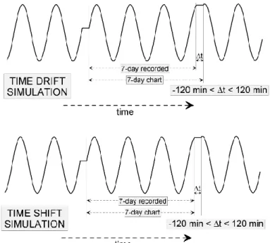
Fig. 1. Scheme of time drift and time shift simulations.
Laboratory, United Kingdom (Bell et al., 2000). A few ques-tions will be addressed and hopefully answered in the paper: How much do computed tides vary in time? Are the changes in tidal amplitudes and phases driven by physical processes or they are artificially induced throughout the measurements and digitising procedure, and (iii) are artificial errors pre-dominant the result of the measurements or of the digitis-ing process? The latter question will include the finddigitis-ings achieved through simulations of time drifts and shifts in the series, both being documented by the tide gauge operators, which will help in answering of the last two questions.
2 Material and methods
Tide gauge at Split was reinstalled in 1954 (the first instal-lation was in 1929), by putting a float-type chart recording device into the stilling well. Two years later, the instrument was replaced with a more precise OTT device, enabling the accuracy in sea level height to be smaller than 1 cm. This de-vice is still operational, although it has been upgraded with a high-precision shaft encoder in 2003. The charts have been changed weekly, and digitised on a monthly basis, in order to obtain hourly sea level values and high/low waters. The most common errors in the system reported by the operators were generated by the clock errors (drift in time), wrong po-sitioning of the pen and the broad trace of the pen line when replacing charts (shift in time), and by the elongation of the charts due to different atmospheric conditions (temperature, air humidity) in the tide gauge location, compared to the cen-tral storeroom (drift in time).
The digitising of the charts has been performed using two different software packages: (1) the charts from 1978 to 2001 were digitised on an older VAX system, with old FORTRAN software which did not allow one to control and change the digitised values during the digitising process, and therefore the data is supposed to be more prone to digitising errors, and (2) the charts older than 1978 were digitised recently using a PC-based package, which consists of an AutoCAD digitising package, a dxf-xyz conversion program and a FORTRAN-based program which calculates the same parameters (hourly values, high/low data) and produces the same data files as the older package. The resolution of both packages is on a 1-cm level, keeping the original accuracy of the measure-ments in the sea level data. The latter package allows for direct changes of digitised curves if necessary, and therefore it is expected to result in more accurate data than the older one. Apart from measurement errors both drifting and shift-ing errors have been reported by the operators to occur durshift-ing digitising, the first being common for the VAX-based soft-ware and the second appearing within the AutoCAD-based software.
The calculation of harmonic constants was performed on annual data files, as it is necessary to have a sufficient length of time series to produce the correct amplitudes and phases of the harmonic constituents (Bell et al., 2000). Seven signif-icant constituents were incorporated into analysis performed by TASK package (Bell et al., 2000), namely semidiurnal M2, S2, K2, N2and diurnal K1, O1and P1tides (Shureman, 1941; Pugh, 1987), which were recognized to be significant in the Adriatic Sea (e.g. Polli, 1960). As year-to-year varia-tions are found both in amplitudes and phases, correlation to
Fig. 2. Annual amplitudes and phases of diurnal constituents
calcu-lated for Split in the 1957–2001 period.
the mean sea level (MSL) has been computed as being one of the factors that may change the tides in a coastal region (Lane, 2004). The nodal tide influence (18.6 years, Shure-man, 1941) on the diurnal and semidiurnal tides is incorpo-rated in the TASK software through scaling with a nodal fac-tor; therefore, no such oscillations can occur in the tides com-puted. In addition, no changes in the surrounding topography (dredging, major constructions, etc.) have been reported in the region, which may influence the tides in the Split Har-bour.
Apart from natural variations, two idealized simulations were constructed, in order to validate the influence of time drifts and shifts on the characteristics of harmonic con-stituents, which were reported by the tide gauge operators and data analysis experts (Hydrographic Institute, personal communication). The first run was based on the assumption that each weekly sea level record is stretched or shrunk in time (Fig. 1a), due to clock errors or elongation of a chart due to humidity and temperature changes, with the weekly drift rate varying from –120 to 120 min (120 min is about 8 mm on a 70-cm weekly chart). The second run was car-ried out assuming that the clock time was correct, but with an offset (shift) between the weekly records from –120 to
Fig. 3. Annual amplitudes and phases of semidiurnal constituents
calculated for Split in 1957–2001 period.
120 min, due to the wrong positioning of the pen on a chart or due to the errors in digitising of the charts (Fig. 1b). There-fore, the cumulative timing error due to a drift may be up to ±480 min in a month. Both artificial records were put in the right position in time every 4 weeks (one month), in order to simulate the digitising process which had been done on a monthly basis. As a result, annual synthetic sea level series were constructed, serving as input to the harmonic analysis. Such a procedure resulted in changes in amplitude and phase of the harmonic constituents due to the time drift and shift, compared to the “regular” time series (no shift and drift), and therefore it will be useful within the error analysis of the measured sea level series.
3 Results
3.1 Data analysis
Figures 2 and 3 show the time series of annual amplitudes and phases of all harmonic constituents, calculated at Split, for the period 1957–2001. The series are split into three sub-series: T1 stands for the records where the changes to the
1486 I. Vilibi´c: The influence of digitisation and timing errors of tidal components at Split
Fig. 4. Mean sea level (MSL) and amplitudes and phases of major
M2and K1 tides between 1986 and 1995, computed on the data
obtained by the VAX (old) and the AutoCAD (new) software.
charts were not done at the regular time, and therefore the accuracy of the sea level data in time is lower, while T2 and T3 represent periods when the charts were changed regularly and the time positioning of data is more correct. The differ-ence between T2 and T3 is in the digitising process; namely, T2 charts were digitised using recently developed PC-based software (AutoCAD) and the drifts in time are minimized, contrary to the T3 charts, which were digitised using an older VAX package, thereby being more prone to errors within the digitising process. The average amplitudes and phases, to-gether with standard deviations are listed in Table 1.
The difference between the constants seems to be rather significant. For example, amplitudes are the lowest in the T1
period (except of N2tide), opposite that of the phases which are commonly the largest in the T1 period (except of K2). Additionally, the T1 period is characterized by the highest standard deviations. Therefore, the data possesses the lowest quality in the T1 period, which is a logical consequence of the irregular changing of a chart and cannot be bridged by digitising, due to a lack of accurate timing information. The amplitudes in the T3 period are even a bit higher, whereas the phases are lower compared to the T2 period. However, all of the amplitudes seem to be lower than the ones documented by ˇSigud (1973). The changes in the semidiurnal amplitudes and phases between the periods are at least two times larger than those of the diurnal ones. For example, the change in the M2amplitude and phase is 22% (1.31 cm) and 24.9◦between the T2 and T1 periods, respectively, whereas the respective change in the K1 amplitude and phase is 6% (0.50 cm) and 12.7◦. Therefore, one can suspect that the drift and shift er-rors occurred at the charts or during the digitising process, as semidiurnal tides are more sensitive to such errors than the diurnal ones, due to their smaller period.
Although the T2 period has lower standard deviations in both amplitudes and phases than the T3 period, the qual-ity of the software packages may be ranked only when analysing the same period by both packages. Therefore, newer AutoCAD-based software has been applied on the 1986–1995 charts, and new tidal amplitudes and phases have been computed (Table 2) and compared to the old ones. First and foremost, new software gives a bit higher amplitudes and lower standard deviations, of which the latter is the proof that the AutoCAD-based software is more accurate and results in better quality sea level data. Also, larger amplitudes mean that less drifting and shifting errors occurred in time, keep-ing more energy on the tidal frequencies (see next section). Large data errors do not occur constantly; they are focused in some years, such as 1993, when both M2and K1tides were recomputed with a 3–4 mm larger amplitude (Fig. 4). Similar characteristics may be concluded for the phase behaviour – both software packages have the same outcome with corre-lated changes in the 1986–1993 period, but they give differ-ent results in 1994 and 1995 (the respective M2and K1phase differences are about 12◦ and 6◦in 1995). Obviously, time drifting and shifting during the digitising process are mostly likely responsible.
Even though it may be concluded that the AutoCAD soft-ware gives more accurate data, some variations in amplitudes and phases may be found in the T2 period (and in the newly computed values in the 1986–1995 period). They may be a result of inaccuracy and errors in data processing which are still largely present in the AutoCAD software (although being lower than in the VAX software), or may be a result of real tidal changes in the region induced by various dy-namical processes (changes in MSL, dredging, building of piers, baroclinic effects, etc.). The changes in the surround-ing bathymetry did not occur in the region in the examined period (Hydrographic Institute of the Republic of Croatia,
Table 1. Average amplitudes and phases, together with standard deviations calculated for T1, T2 and T3 periods. The constituents given by
ˇSigud (1973) are shown, too.
Table 1. M2 S2 K2 N2 K1 O1 P1 H (cm) g (o) H (cm) g (o) H (cm) g (o) H (cm) g (o) H (cm) g (o) H (cm) g (o) H (cm) g (o) Šigud (1973) 7.95 129.0 5.58 130.8 1.64 124.1 1.38 125.6 8.82 55.9 2.69 47.5 2.90 51.8 T1 period 6.06 ± 0.55 161.0 ± 5.2 4.02 ± 0.58 162.8 ± 4.0 1.43 ± 1.16 127.2 ± 69.9 1.36 ± 0.16 168.2 ± 7.4 7.94 ± 0.21 73.9 ± 2.4 2.53 ± 0.18 59.2 ± 3.0 2.76 ± 0.94 72.6 ± 9.2 T2 period 7.37 ± 0.36 136.1 ± 3.9 5.17 ± 0.21 138.3 ± 4.3 1.55 ± 0.21 135.6 ± 6.7 1.18 ± 0.10 137.0 ± 9.3 8.44 ± 0.25 61.2 ± 2.4 2.64 ± 0.11 48.5 ± 3.0 2.88 ± 0.18 56.4 ± 4.3 T3 period 7.56 ± 0.46 123.6 ± 8.4 5.37 ± 0.25 125.7 ± 7.1 1.72 ± 0.20 122.0 ± 9.3 1.26 ± 0.14 124.2 ± 10.6 8.47 ± 0.40 52.8 ± 5.3 2.73 ± 0.23 42.6 ± 7.2 2.86 ± 0.27 49.0 ± 7.5 Table 2. M2 S2 K2 N2 K1 O1 P1 H (cm) g (o) H (cm) g (o) H (cm) g (o) H (cm) g (o) H (cm) g (o) H (cm) g (o) H (cm) g (o) 1986-1995 old 7.82 ± 0.34 125.5 ± 3.7 5.45 ± 0.22 126.8 ± 3.9 1.77 ± 0.21 124.0 ± 6.1 1.30 ± 0.15 127.8 ± 7.9 8.65 ± 0.20 54.3 ± 1.8 2.76 ± 0.10 44.7 ± 5.8 2.91 ± 0.14 48.9 ± 4.2 1986-1995 new 7.86 ± 0.20 127.6 ± 2.9 5.51 ± 0.15 129.3 ± 3.2 1.78 ± 0.16 127.1 ± 4.6 1.22 ± 0.13 129.4 ± 8.8 8.73 ± 0.12 55.1 ± 1.6 2.81 ± 0.11 44.5 ± 4.1 3.00 ± 0.22 49.6 ± 4.0
Table 2. Average amplitudes and phases, together with standard deviations calculated for 1986–1995 by using old VAX and new
AutoCAD-based software. Table 1. M2 S2 K2 N2 K1 O1 P1 H (cm) g (o) H (cm) g (o) H (cm) g (o) H (cm) g (o) H (cm) g (o) H (cm) g (o) H (cm) g (o) Šigud (1973) 7.95 129.0 5.58 130.8 1.64 124.1 1.38 125.6 8.82 55.9 2.69 47.5 2.90 51.8 T1 period 6.06 ± 0.55 161.0 ± 5.2 4.02 ± 0.58 162.8 ± 4.0 1.43 ± 1.16 127.2 ± 69.9 1.36 ± 0.16 168.2 ± 7.4 7.94 ± 0.21 73.9 ± 2.4 2.53 ± 0.18 59.2 ± 3.0 2.76 ± 0.94 72.6 ± 9.2 T2 period 7.37 ± 0.36 136.1 ± 3.9 5.17 ± 0.21 138.3 ± 4.3 1.55 ± 0.21 135.6 ± 6.7 1.18 ± 0.10 137.0 ± 9.3 8.44 ± 0.25 61.2 ± 2.4 2.64 ± 0.11 48.5 ± 3.0 2.88 ± 0.18 56.4 ± 4.3 T3 period 7.56 ± 0.46 123.6 ± 8.4 5.37 ± 0.25 125.7 ± 7.1 1.72 ± 0.20 122.0 ± 9.3 1.26 ± 0.14 124.2 ± 10.6 8.47 ± 0.40 52.8 ± 5.3 2.73 ± 0.23 42.6 ± 7.2 2.86 ± 0.27 49.0 ± 7.5 Table 2. M2 S2 K2 N2 K1 O1 P1 H (cm) g (o) H (cm) g (o) H (cm) g (o) H (cm) g (o) H (cm) g (o) H (cm) g (o) H (cm) g (o) 1986-1995 old 7.82 ± 0.34 125.5 ± 3.7 5.45 ± 0.22 126.8 ± 3.9 1.77 ± 0.21 124.0 ± 6.1 1.30 ± 0.15 127.8 ± 7.9 8.65 ± 0.20 54.3 ± 1.8 2.76 ± 0.10 44.7 ± 5.8 2.91 ± 0.14 48.9 ± 4.2 1986-1995 new 7.86 ± 0.20 127.6 ± 2.9 5.51 ± 0.15 129.3 ± 3.2 1.78 ± 0.16 127.1 ± 4.6 1.22 ± 0.13 129.4 ± 8.8 8.73 ± 0.12 55.1 ± 1.6 2.81 ± 0.11 44.5 ± 4.1 3.00 ± 0.22 49.6 ± 4.0
private communication). On the other hand, the changes in MSL are correlated with the changes in some tidal ampli-tudes on the 95% level (Fig. 5), but not for other ampliampli-tudes and not for all of the tidal phases. Furthermore, most of the AutoCAD-computed amplitudes in 1986–1995 are cor-related with the VAX-computed amplitudes (Fig. 6), which is predominantly a result of the errors that occurred during the measurements which cannot be improved by the digitis-ing software. Therefore, the lower variance obtained by Au-toCAD software is the result of the improvement of the digi-tising process and the lowering of the artificial errors there. Conclusively, some improvement in sea level data quality can be made by improving the digitising software, but only to the level limited by the errors acquired through the measurement processes which cannot be resolved and corrected during the reanalysis.
3.2 Time drift and shift simulations
Simulated changes in constituent amplitudes and phases due to the artificial drift and shift in the time series (see Fig. 1 and Sect. 2) are shown in Fig. 7. One can see that the changes in amplitude are not so pronounced as the changes in phase, both for semidiurnal and diurnal constituents, be-ing almost linearly shifted in the same direction as the con-structed time series. If the drift is large enough, semidiurnal amplitudes decrease rather rapidly, for about 4% for a drift rate of ±120 min. This is equivalent to about 3 mm for the
M2tide or about 2 mm for the S2tide, which is still signif-icantly lower than the standard deviation in all of the exam-ined periods (Tables 1 and 2). The drift impacts tidal phases quite a lot versus the observed variability; this is due to the fact that each sea level chart can be drifted with a different value. The changes in diurnal tides are significantly lower; K1decreases only 1 mm if the drift is 120 min. A small ex-ception is the P1tide, which increases in amplitude when the drift rate is negative. Such behaviour is a result of artificial energy transfer from the K1to the P1tide, as the K1tide has a period rather close to P1(23.93 h of K1versus 24.07 h of P1).
The simulations in time shift (Fig. 8) resulted in a somewhat different behaviour of the harmonic constituents, namely, the M2and S2tides (which have large amplitudes) behave similarly as in the time drift simulations, whereas the K2and N2tides have larger amplitudes when the drift is neg-ative, and smaller ones when the drift is positive. In partic-ularly, N2values vary from 200% down to 10% of the non-shifted simulation, obviously due to the influence of a larger M2 tide. The drift of ±120 min generates the decrease in the M2and S2tides for about 10% (8 mm for M2, 5 mm for S2), whereas the of that drift (±60 min) results in decrease of about 3–4% (2–3 mm for M2, 2 mm for S2). Diurnal tides are more stable again, changing their amplitudes up to 4% from the real (non-shifted) one (3 mm for K1).
1488 I. Vilibi´c: The influence of digitisation and timing errors of tidal components at Split
Fig. 5. Regression diagrams between MSL and the M2and K1
am-plitudes (Hnew)obtained by the AutoCAD software between 1986
and 1995.
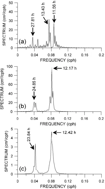
All of these simulations result in increased “false” energy in the domain of tidal frequencies (Fig. 9). False energies are larger for semidiurnal tides, in accordance with the changes in phases and amplitudes calculated from the real sea level data. They are also larger for time shift errors rather than time drift, due to the cumulative error effect in a month. The period of false maximums don’t coincide with the tidal peri-ods for the regular simulations (time drift and shift rate are constant). Nevertheless, the tidal energy is not recognized by the harmonic analysis in the case of the variable (ran-dom) rates, both in time drifts and shifts (Fig. 9c), and the remaining residual sea level series has a maximum exactly on the tidal periods (12.42 – M2tide, 23.83 – K1tide). This “false” energy, generated by the measuring and digitising er-rors, seems to be persistent in a number of sea level studies (e.g. Ceroveˇcki et al., 1997; Raicich et al., 1999; Pasari´c and Orli´c, 2001; Vilibi´c, 2006), although it has been assumed there that a nonlinear coupling between the internal and sur-face tides and seiches might be responsible. However, this
coupling has not been captured or modelled yet, leading to the conclusion that: (i) it is very weak or absent, and the residual energy at the M2and K1periods is a product of drift-ing and shiftdrift-ing errors in the sea level series, or (ii) it may be strong and dominant, but a part of the energy at these periods is surely the result of the errors in the sea level series.
4 Conclusions
The knowledge of harmonic constituents is essential when making tidal forecasts, as the rate of sea level changes serves as input in various activities dealing with the sea and coastal infrastructure (Vilibi´c et al., 2000). For example, sea level data is used within the various hydrotechnical projects, on offshore drilling platforms, in the charting and naviga-tion safety studies, when building coastal infrastructure, etc. Therefore, determination of the tidal signal and the calcu-lation of the harmonic constituents at one long-term station has been performed in this work, and the interannual variabil-ity is detected and discussed in the light of (i) measurement errors (clock errors, chart stretching due to changes in tem-perature and humidity, etc.), (ii) various digitising software packages that were changed over the period of operation (old VAX-based software versus new AutoCAD-based software), and (iii) natural changes induced by changes in MSL and bathymetry (dredging, etc.). A few conclusions may be ex-tracted from the analyses in this paper:
– Semidiurnal tides possess larger variance than diurnal
ones, being more prone to artificial errors in the sea level series. In addition, artificial errors usually decrease the amplitudes of a tide, as some of the tidal energy is trans-ferred to the residual (de-tided) sea level series.
– Most of the observed changes in tidal amplitudes and
phases come from artificially generated errors in the data, although some weak correlation is computed be-tween some tidal amplitudes and the MSL (e.g. for the M2tide). Based on that correlation (Fig. 5), an increase of 3 cm in the M2 amplitude may be expected for the MSL rise of 50 cm, however, a numerical model should be applied in order to properly quantify this. There-fore, MSL variations have an effect on tides, but they can be hardly resolved from the data due to artificial er-rors. Other natural effects (e.g. dredging, building of piers, etc.) have a negligible effect on the tides, as these activities were not documented to occur in the wider re-gion during the tide gauge operation.
– The upgrade of the digitising software decreased the
er-rors being generated through the digitising process and increased the quality of the sea level data; however, some errors still remained in the series, mostly includ-ing the errors created durinclud-ing the measurements (clock and pen positioning, chart stretching).
Fig. 6. Regression diagrams between the VAX-computed (Hold, gold)and AutoCAD-computed (Hnew, gnew)amplitudes and phases between
1490 I. Vilibi´c: The influence of digitisation and timing errors of tidal components at Split
Fig. 7. Simulated changes in relative amplitudes and phase differences versus the time drift rate. The respective amplitude and phase are
supposed to be 1 and 0 when no time drift was simulated.
Fig. 8. Simulated changes in relative amplitudes and phase differences versus the time shift rate. The respective amplitude and phase are
supposed to be 1 and 0 when no time shift was simulated.
– The errors that were created by artificial drifting and/or
shifting of a chart in time may result in “false” resid-ual energy on tidal frequencies. In particular, artificial energy at the M2period (12.4 h) has been documented in a large number of previous sea level studies, hypoth-esised to be a result of the nonlinear effects between
tides, internal tides and seiches. However, the energy may be the result of drifting and shifting errors in sea the level series rather than of natural origin, which should be checked in the future through modelling studies.
Fig. 9. Spectrum of the annual residual series computed from the
simulated sea level series with (a) a time drift of 30 min, (b) a time shift of 30 min, and (c) a time drift randomly chosen for each artifi-cial chart (week) with values between –120 and 120 min.
Acknowledgements. A part of sea level charts has been digitised
within ESEAS-RI project (EU funded project EVR1-CT-2002-40025). Half-century maintenance of the Split tide gauge carried out by personnel of Hydrographic Institute of the Republic of Croa-tia is particularly appreciated. The Permanent Service for Mean Sea Level kindly provided TASK software package, S. ˇCupi´c did quite great job with digitising of sea level charts, while M. Srdeli´c devel-oped PC-based digitising software.
Topical Editor N. Pinardi thanks a referee for his help in evalu-ating this paper.
References
Bell, C., Vassie, J. M., and Woodworth, P. L.: POL/PSMSL Tidal Analysis Software Kit 2000 (TASK-2000), Permanent Service for Mean Sea Level, CCMS Proudman Oceanographic Labora-tory, Bidston, 21 pp, 2000.
Ceroveˇcki, I., Orli´c, M., and Hendershott, M. C.: Adriatic seiche decay and energy loss to the Mediterranean, Deep-Sea Research I, 44, 2007–2029, 1997.
Chapalain, G. and Thais, L.: Tide, turbulence and suspended sed-iment modelling in the eastern English Channel, Coastal Engi-neering, 41, 295–316, 2000.
Kasumovi´c, M.: Harmonic analysis of tides at Bakar (in Croa-tian), Geofizi`eki institut Prirodoslovno-matemati`ekog fakulteta Sveuˇciliˇsta u Zagrebu, Radovi III/1, Zagreb, 1–9, 1952. Lane, A: Bathymetric evolution of the Mersey Estuary, UK, 1906–
1997: causes and effects, Estuarine Coastal and Shelf Sciences, 59, 249–263, 2004.
Pasari´c, M. and Orli´c, M.: Long-term meteorological precondition-ing of the North Adriatic coastal floods, Continental Shelf Re-search, 21, 263–278, 2001.
Polli, S.: Le propagazione delle maree nell’ Adriatico (in Ital-ian), Atti del IX Convegno dell’ Associazione Geofisica Italiana, Roma, 1–11, 1960.
Prandle, D.: Operational oceanography in coastal waters, Coastal Engineering, 41, 3–12, 2000.
Pugh, D. T.: Tides, Surges and Mean Sea Level, John Wiley, Chicester, 472 pp, 1987.
Raicich, F., Orli´c, M., Vilibi´c, I., and Malaˇciˇc, V.: A case study of the Adriatic seiches (December 1997), Il Nuovo Cimento C, 22, 715–726, 1999.
Robinson, A. R., Tomasin, A., and Artegiani, A.: Flooding of Venice – phenomenology and prediction of the Adriatic storm surge, Quart. J. Roy. Meteorol. Soc., 99, 686–692, 1972. Shureman, P.: Manual of Harmonic Analysis and Prediction of
Tides, US Department of Commerce, Special Publication No 98, Washington, 317 pp, 1941.
ˇSigud, J.: Tide tables, Adriatic Sea – east coast – 1974 (in Croatian), Hydrographic Institute, Split, 1973.
UNESCO: Manual on sea level measurement and interpretation, Volume I – Basic procedures, IOC Manuals and Guides 14, UN-ESCO, 83 pp, 1985.
Vilibi`c, I.: The role of the fundamental seiche in the Adriatic coastal floods, Continental Shelf Research, 26, 206–216, 2006. Vilibi`c, I., Leder, N., and Smirˇciˇc, A.: Storm surges in the Adriatic
Sea: an impact on the coastal infrastructure, Periodicum Biolo-gorum, 102, Supplement 1, 483–488, 2000.