HAL Id: hal-00317838
https://hal.archives-ouvertes.fr/hal-00317838
Submitted on 28 Jul 2005
HAL is a multi-disciplinary open access
archive for the deposit and dissemination of
sci-entific research documents, whether they are
pub-lished or not. The documents may come from
teaching and research institutions in France or
abroad, or from public or private research centers.
L’archive ouverte pluridisciplinaire HAL, est
destinée au dépôt et à la diffusion de documents
scientifiques de niveau recherche, publiés ou non,
émanant des établissements d’enseignement et de
recherche français ou étrangers, des laboratoires
publics ou privés.
patterns, and a possible cause
L. G. Blomberg, J. A. Cumnock, I. I. Alexeev, E. S. Belenkaya, S. Yu.
Bobrovnikov, V. V. Kalegaev
To cite this version:
L. G. Blomberg, J. A. Cumnock, I. I. Alexeev, E. S. Belenkaya, S. Yu. Bobrovnikov, et al.. Transpolar
aurora: time evolution, associated convection patterns, and a possible cause. Annales Geophysicae,
European Geosciences Union, 2005, 23 (5), pp.1917-1930. �hal-00317838�
SRef-ID: 1432-0576/ag/2005-23-1917 © European Geosciences Union 2005
Annales
Geophysicae
Transpolar aurora: time evolution, associated convection patterns,
and a possible cause
L. G. Blomberg1, J. A. Cumnock1,2, I. I. Alexeev3, E. S. Belenkaya3, S. Yu. Bobrovnikov3, and V. V. Kalegaev3
1Alfv´en Laboratory, Royal Institute of Technology, Stockholm, Sweden 2Center for Space Sciences, University of Texas at Dallas, USA
3Skobeltsyn Institute of Nuclear Physics, Moscow State University, Russia
Received: 22 April 2004 – Revised: 11 May 2005 – Accepted: 17 May 2005 – Published: 28 July 2005
Abstract. We present two event studies illustrating the
de-tailed relationships between plasma convection, field-aligned currents, and polar auroral emissions, as well as illustrat-ing the influence of the Interplanetary Magnetic Field’s y-component on theta aurora development. The transpolar arc of the theta aurorae moves across the entire polar region and becomes part of the opposite side of the auroral oval. Elec-tric and magnetic field and precipitating particle data are pro-vided by DMSP, while the POLAR UVI instrument provides measurements of auroral emissions. Ionospheric electrostatic potential patterns are calculated at different times during the evolution of the theta aurora using the KTH model. These model patterns are compared to the convection predicted by mapping the magnetopause electric field to the ionosphere using the Paraboloid Model of the magnetosphere. The model predicts that parallel electric fields are set up along the magnetic field lines projecting to the transpolar aurora. Their possible role in the acceleration of the auroral electrons is discussed.
Keywords. Ionosphere (Plasma convection; Polar
iono-sphere) – Magnetospheric physics (Magnetosphere-ionosphere interactions)
1 Introduction
The global distribution of the aurora has a qualitative as well as a quantitative dependence on the interplanetary magnetic field (IMF). For southward IMF the intense auroral activ-ity is usually confined to the region known as the auroral oval, whereas for northward IMF considerable auroral activ-ity is often encountered poleward of this region (e.g. Davis, 1963; Berkey et al., 1976; Lassen and Danielsen, 1978). The existence of auroral arcs at very high latitudes was es-tablished early on (e.g. Mawson, 1916; Davis, 1960; Den-holm, 1961; Denholm and Bond, 1961; Eather and
Aka-Correspondence to: L. G. Blomberg
sofu, 1969). These arcs, variably referred to in the litera-ture as “Sun-aligned arcs,” “polar cap arcs,” “high-latitude arcs,” and “polar arcs,” have been observed for many years using all-sky cameras (e.g. Lassen and Danielsen, 1978), and photometers on board low-altitude polar-orbiting spacecraft, such as ISIS and DMSP (e.g. Gussenhoven, 1982; Ismail and Meng, 1982; Hoffman et al., 1985). However, due to the lim-ited view of all-sky cameras and photometers on low-altitude satellites, these arcs were considered relatively isolated fea-tures. It was not until imaging instruments were flown on high-altitude spacecraft, such as Dynamics Explorer 1 (e.g. Frank et al., 1982, 1986) and Viking (e.g. Murphree et al., 1987), that the existence of so-called transpolar arcs (TPAs), luminous features extending across the polar region linking the dayside aurora to the nightside oval, became clear. A comprehensive overview of observations related to polar arcs and their electrodynamics is found in Blomberg and Mark-lund (1993). Valladares et al. (1994) performed a compre-hensive statistical study of the occurrence of high-latitude arcs and their dependence on the IMF. Recently, Kullen et al. (2002) extended the Gussenhoven (1982) classification of polar arcs and presented statistics of the different arc types based on three months of POLAR UVI observations. Sev-eral models have been created attempting to explain transpo-lar arcs (e.g. Chang et al., 1998; Newell et al., 1999; Kullen, 2000; Slinker et al., 2001; Kullen and Janhunen, 2004; Naehr and Toffoletto, 2004). However, since not all polar arcs are transpolar, care must be taken not to confuse the different types when discussing their occurrence, the corresponding magnetospheric topology, or the physical mechanisms caus-ing them.
Transpolar arcs form, in the Northern Hemisphere, from an expanded dawnside (duskside) emission region when
By changes from negative to positive (positive to negative) (Cumnock et al., 1997, Cumnock et al., 2002). If the IMF re-mains sufficiently stable after the initial By polarity change, the transpolar arc will usually migrate across the polar re-gion, often in both hemispheres (Cumnock, 2005). The pat-tern commonly referred to as the theta aurora describes the
situation when a transpolar arc is aligned nearly along the noon-midnight meridian (Frank et al., 1986). The TPAs cross the noon-midnight meridian only when Bychanges sign, re-sulting in a large Bz/|By|ratio. The focus of the present paper is on moving transpolar arcs, i.e., large-scale arcs traversing the entire polar region in response to a Bychange, forming a theta aurora when the arc is at highest latitude.
Ionospheric convection patterns observed during north-ward IMF generally contains regions of sunnorth-ward flow at highest latitudes, in contrast to the antisunward flow prevail-ing for southward IMF. A variety of configurations have been used to explain these observations, including spatially dom-inant one-cell patterns and multiple-cell patterns. The num-ber of cells seems to have a first-order dependence on the ratio of Bz to By, resulting in an increasing number of cells and reverse convection at highest latitudes as the IMF be-comes more strongly northward (Potemra et al., 1984; Reiff and Burch, 1985; Heelis et al., 1986; Cumnock et al., 1995; Cumnock and Blomberg, 2004, and references therein). Ob-servations indicate that TPAs may be associated with either sunward or antisunward flow, as well as a variety of con-vection patterns, including a four-cell pattern (Frank et al., 1986; Gusev and Troshichev, 1990; Jankowska et al., 1990; Zanetti et al., 1990), a dominant one-cell (Hoffman et al., 1985), a three-cell ( Carlson et al., 1988; Zanetti et al., 1990; Jankowska et al., 1990), or a distorted two-cell (Robinson and Mende, 1990; Marklund et al., 1991). These studies are all based on isolated observations of single TPAs and thus represent different stages of theta aurora evolution relating to changing IMF Bxand Byconditions during northward IMF. Satellites have observed a variety of field-aligned current (FAC) configurations, including pairs of upward and down-ward field-aligned current sheets associated with the TPAs (e.g. Frank et al., 1986; Menietti and Burch, 1987; lund et al., 1991; Obara et al., 1993; Blomberg and Mark-lund, 1993; Blomberg and Cumnock, 2005). In addition, as the IMF becomes more northward both the Region 1 to Re-gion 2 and the NBZ to ReRe-gion 1 current ratios increase (e.g. Blomberg and Marklund, 1993).
The main purpose of this paper is to model the global po-tential patterns and to compare them to the convection pre-dicted by mapping the magnetopause electric field to the ionosphere using the Paraboloid Model of the magnetosphere during the evolution of dawnside and duskside originating transpolar arcs. The present study follows up on the results of Cumnock and Blomberg (2004). Utilizing satellite data, the Royal Institute of Technology (KTH) numerical model pro-vides the high-latitude global potential pattern. In addition, the magnetopause electric field predicted from IMF data is mapped to the ionosphere using Moscow State University’s (MSU) Spherical and Paraboloid Models of the magneto-sphere.
We model the entire evolution of the theta aurorae, and compare observations to the output of both models. In both events the transpolar arc moves across the entire polar region and eventually becomes part of the opposite side of the auro-ral oval.
2 Observations and model results
The Ultraviolet Imager (UVI) experiment (Torr et al., 1995) on the POLAR spacecraft provides global images of the au-rora. The instrument is able to resolve 0.5 deg in latitude at apogee; thus, a single pixel projected to 100 km altitude from apogee is approximately 50×50 km. In the Lyman-Birge-Hopfield mode (LBH) the instrument measures molecular ni-trogen emissions in the 140–160 nm spectral region.
The Defense Meteorological Satellite Program’s (DMSP) satellites provide measurements of precipitating particles and ionospheric plasma flows from three Northern Hemisphere passes during each of the two time periods of interest. DMSP F13 (Rich, 1994) passes in the dusk-to-dawn direction and DMSP F14 from about 21 MLT to 10 MLT in the Northern Hemisphere. The electrostatic potential distribution is de-rived by integrating the electric field (E) along the satellite track, utilizing E=−v×B, where v is the measured trans-verse ion drift velocity and (B) is the model geomagnetic field. The electrostatic potential can then be used to deter-mine which regions of sunward and antisunward flow may be connected by equipotential flow lines.
In order to analyse the global potential patterns during theta aurora evolution we utilize the KTH numerical model that assumes a field-aligned current distribution and a con-ductivity model and from these calculates the potential dis-tribution. A detailed description of the model is found in Blomberg and Marklund (1991a). The model input (the field-aligned current distribution) is qualitatively inferred from satellite UV images that give direct information about up-ward currents associated with electron precipitation. Down-ward currents are qualitatively inferred from statistical mod-els. The currents are then quantitatively calibrated directly against satellite magnetometer data, as well as indirectly cal-ibrated by comparing the calculated model potential pattern to satellite plasma flow data in an iterative manner. Data from one or more satellites can be used for the calibration, here DMSP F13 and F14 data were used.
The polar cap convection dependence on the IMF direction may be estimated by mapping the solar wind electric field to the polar ionosphere (Alexeev, 1986; Toffoletto and Hill, 1989). This approach assumes a very high conductivity along the magnetospheric magnetic field and thus magnetic field lines are equipoential. In this model, global reconfiguration of the magnetospheric magnetic field leads to modification of the polar cap convection (Belenkaya, 1998a,b; 2002).
The goal here is to reconstruct on a global scale the dis-tribution of all auroral electrodynamic parameters during the evolving northward IMF conditions as a TPA moves across the entire polar region. Model inputs are the ionospheric conductivity and FAC distributions. The boundary condition used is that the potential is zero at 50◦ magnetic latitude; in reasonable agreement with DMSP data. Model output is the ionospheric potential that can be compared with the po-tential calculated from electric field data along the DMSP satellite tracks. POLAR UVI provides information on the upward FAC distribution. For more details on UVI, DMSP
and the KTH numerical model for the events discussed here, see Cumnock and Blomberg (2004).
2.1 Spherical model of the magnetosphere
In the Moscow State University spherical model of the Earth’s magnetosphere (Alexeev and Belenkaya, 1983), the magnetopause is approximated by a sphere of radius
R1=10RE with the geomagnetic dipole located in its cen-tre. At the magnetopause there are screening currents that create a uniform magnetic field antiparallel to the dipole mo-ment. The magnetic field b that penetrates from the solar wind into the magnetosphere is b=kB, where B is the in-terplanetary magnetic field (IMF) and k≈0.1. The spherical model describes the general features of the interaction be-tween the interplanetary and magnetospheric fields. In the dayside magnetosphere and in the polar caps the model out-put is consistent with observations.
The magnetic field associated with the magnetopause screening currents allows us to distinguish between two dif-ferent types of reconnection, corresponding to southward and northward IMF (Alexeev and Belenkaya, 1983). For southward IMF (Bz<0), two-dimensional reconnection takes place at the merging line on the spherical magnetopause. Figure 1 shows the meridional cross section of the spheri-cal magnetosphere for southward IMF. The region marked 1 indicates closed field lines, the regions 2a and b (dotted) indicate open field lines of the northern and southern po-lar caps. For northward IMF (Bz>0), three-dimensional re-connection occurs at the two neutral magnetic field points. Figure 2 shows the meridional cross section of the spheri-cal magnetosphere for northward IMF. The region marked 1 indicates closed field lines, the regions 2a and b (dotted) indicate open field lines of the northern and southern polar caps, and the shaded region indicates interplanetary mag-netic field lines inside the magnetosphere. The neutral points and neutral lines are surrounded by diffusion regions where the conductivity is high but finite and where MHD breaks down. Magnetic field lines outside of the diffusion regions are assumed to be equipotential. This assumption, together with the boundary condition for the electric field component tangential to the magnetopause: Et=kEI MF, gives us the electric potential distributions in the open field line regions, where E is the fraction of the solar wind electric field EI MF that penetrates into the magnetosphere.
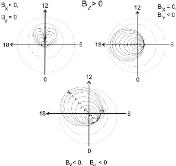
The spherical magnetospheric model was used to calculate distributions of the electrostatic potential in the open field line region in the northern ionosphere. The electrostatic po-tential distributions in the northern polar cap, predicted by the spherical model, are shown for southward IMF in Fig. 3 and for northward IMF in Fig. 4 (see also (Belenkaya, 1998a, b). For both cases k=0.1 was assumed. For northward IMF, the ionospheric convection pattern on the open field lines has two cells for Bx6=0 and one cell for Bx=0, By6=0. Reverse convection occurs near the cusp projection.
Figure 5 (derived from Fig. 9 of Cowley (1973)) illustrates the three-dimensional geometry of the superposition of the
Fig. 1. The meridional cross section of the spherical magnetosphere for southward IMF. The region marked 1 indicates closed field lines, the regions 2a and b (dotted) indicate open field lines of the northern and southern polar caps.
Fig. 2. The meridional cross section of the spherical magnetosphere for northward IMF. The region marked 1 indicates closed field lines, the regions 2a and b (dotted) indicate open field lines of the northern and southern polar caps, the shaded region indicate interplanetary magnetic field lines inside the magnetosphere.
dipole and the uniform magnetic fields for northward IMF. In the spherical model the uniform field is simply the sum of the penetrated portion of the IMF and the magnetic field re-sulting from the magnetopause currents screening the dipole field (both of them are also uniform fields). The surfaces A1 and A2 divide magnetic field lines of different topological types (open, closed, and interplanetary) and are called sepa-ratrix surfaces (see, for example, Siscoe et al., 2001). A1 is a boundary between open and interplanetary magnetic field lines, whereas A2 divides open and closed magnetic flux-tubes. Two magnetic field lines connecting the two neutral points (OS and ON)form a separator line (C1C2, part C2is
Fig. 3. Distribution of the electric equipotentials in the open field line region of the northern polar cap, in the spherical model, for southward IMF, B, dependent on bxand by, (b=kB, k=0.1).
Fig. 4. Distribution of the electric equipotentials in the open field line region of the northern polar cap in the spherical model for northward IMF dependent on bxand by.
separator line. For southward IMF (not shown), the sepa-rator line is a quasi-neutral line, since at each point in the plane perpendicular to it, magnetic field lines have an X-type configuration, leading to two-dimensional reconnection. For northward IMF, there is no quasi-neutral line in the magne-tosphere.
For northward IMF, the boundary of the northern open field line bundle, A1, converges to the northern magnetic
Fig. 5. Three-dimensional geometry of the superposition of the dipole and uniform (generated by the magnetopause currents and penetrated from the solar wind) magnetic fields for northward IMF (derives from Fig. 9 of Cowley (1973)).
null ON. The separatrix surface formed by the magnetic field lines originating from the boundary of the southern polar cap also converges to the northern magnetic null. From this null point and perpendicular to both separatrix surfaces, two sin-gular magnetic field lines B1and B2diverge (these singular
lines were called “stemlines” by Siscoe et al. (2001)). Along B2,the neutral point ON maps to the ionospheric projection of the cusp (ON’).
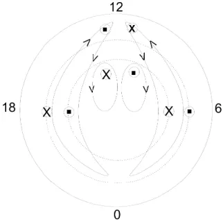
Alexeev and Belenkaya (1985) obtained an analytical ex-pression approximating the NBZ currents on open field lines during northward IMF. NBZ currents flow out of (into) the ionosphere in the dawn (dusk) sectors. These field-aligned currents are each related to a convective vortice: the upward current with a clockwise one and the downward current with an anticlockwise cell. Figure 6 illustrates all field-aligned currents and ionospheric convection flows for Bz>0 (Clauer et al., 2001).
Let us assume for a moment that there are no parallel elec-tric fields, and thus that each magnetic field line is an equipo-tential curve. Then, equipoequipo-tential curves on the intersection of the southern magnetopause with the open field line bun-dle of the northern polar cap project to convection cells in the ionosphere. This is because the whole boundary of the open field line bundle converges to the neutral point ON(see Fig. 5). Each equipotential crosses the open field line bundle boundary at two points. If projected to the ionosphere, these points all end up at ON’, with the single exception being the projection of the equipotential contour which intersects at some point, LN,the singular southern magnetic field line B1.
This contour has a potential 8LN. By analogy, the singular equipotential contour on the magnetopause of the open field lines connecting to the southern polar cap, which intersects
the northern stemline B1at LShas the potential 8LS(LNand LS are located at the intersections of the stemlines B1 with
the magnetopause). The point LN maps along the southern B1 to OS and then along the southern B2 to OS’ and also along A2to the open field line boundary of the northern
po-lar cap. Thus, the boundary of the open field lines in the Northern Hemisphere has a potential 8LN.The projection of the southern cusp OS along the southern stemline B2on the
southern ionosphere (OS’) also has the potential 8LN. Sim-ilarly, ON and ON’ have a potential 8LS which is also the potential of the open field line boundary in the southern polar cap. So, on the northern (southern) equipotential ionospheric boundary between open and closed field lines, a singularity exists, ON’ (OS’), where the potential macroscopically (on the MHD scale) is discontinuous. This exception determines the source function in the Poisson equation for the entire po-lar cap.
We now have magnetic field lines forming the boundary of the open field line bundles, all converging to the null points ON or OS. For these lines the equipotentiality assumption for the magnetic field lines is invalid. Thus, an electric field component parallel to the magnetic field must exist (Greene, 1988) on the field lines of the cylindrical separatrix surfaces. All magnetic field lines of these separatrix surfaces tend to reach closer to the separator line (C1C2)before veering off
to the null points on the magnetopause (Siscoe et al., 2001). The singular equipotential traversing the point LN maps to the open field line region of the northern polar cap, which it divides into two vortices. Its projection has a potential
8LN, except in the vicinity of ON’, where the potential is 8LS. This means that for By6=0 (for which 8LN6=8LS) aligned potential drops and consequently, strong field-aligned currents should exist along those field lines which are topologically connected to the null points (Belenkaya, 2002). The locations of the ionospheric projections of the singular equipotentials (LN’ON’, LS’OS’) dividing the polar caps into two vortices depend on the By component of the IMF (see Fig. 4). For By<0 (By>0) LN’ON’ is in the dawn (dusk) sector of the northern polar cap.
The potential drop δ8=8LN−8LS that exists between the two magnetic nulls for By6=0 also exists on the separa-tor line (C1C2)connecting the two magnetic neutral points.
Siscoe et al. (2001) emphasized the significant role that Ek plays for the global magnetic reconnection. Greene (1988) also mentioned that Ekarises due to the electric field singu-larity at the neutral points of the magnetic field. The potential of LSis
8LS=8ON. (1)
By analogy, the potential
8LN =8OS. (2)
We introduce δ8 as the potential drop between the null points
δ8 = 8LN −8LS=8OS−8ON. (3)
Fig. 6. Field-aligned currents and convection in the polar cap for northward IMF. From high to lower latitudes: NBZ currents, Region I and II currents, currents near the cusp region on the closed field lines (Clauer et al., 2001).
For the spherical model 8OS−8ON=δ8pcsinϕm, where ϕm is the angle between the x-axis and the projection of the IMF-vector on the x-y plane, and δ8pcis the potential drop across the polar cap in the spherical model for southward IMF. ϕm is defined by:
sinϕm=By/Bl,cosϕm=Bx/Blwhere Bl=(Bx2+By2)1/2. (4) For Bx=0 and By6=0, sinϕm=±1 and the potential drop be-tween the magnetic null points maximises and becomes equal to δ8pc. This result agrees with that obtained by Siscoe et al. (2001): for azimuthal IMF the potential drop across the open field line bundle is equal to the potential drop applied to the separator line connecting the two neutral points.
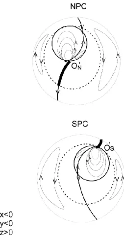
Extending the singular equipotential onto the closed iono-spheric field lines divides the two low-latitude vortices of the four-cell convection system existing for northward IMF. In Fig. 7 the corresponding convection patterns in the northern and southern ionosphere are shown. We see that for Bx<0, closed field lines going near the separator line C1C2(thick
curve) in the Northern Hemisphere are close to the singular equipotential on closed plasma sheet field lines. We assume that a field-aligned potential drop can exist only in the vicin-ity of C1C2. Low-latitude closed field lines located
equator-ward of the poleequator-ward edge of the auroral oval are not affected very much by the IMF. Thus, those lines do not approach C1C2and, consequently, they are equipotential. We therefore
expect the field-aligned potential drop to be on the singular equipotential on the plasma sheet closed field lines from the cusp projection up to the poleward edge of the auroral oval.
We suggest, following Belenkaya (2002), that the auro-ral emissions in transpolar auroauro-ral arcs are caused, largely, by the potential difference that exists between the northern
Fig. 7. Ionospheric convection patterns in the northern and South-ern Hemispheres. Thick curves mark the location of magnetic field lines that come close to the separator line C1C2. Northward IMF with Bx<0, By<0.
and southern magnetic null points for IMF By6=0. On the local scale, the potential difference along a particular mag-netic field line traversing the transpolar arc, determines the acceleration potential. The emission region should further be associated with the singular equipotential on the closed plasma sheet field lines from the cusp projection to the pole-ward boundary of the auroral oval (in the northern polar cap for Bx<0 and in the southern polar cap for Bx>0).
2.2 Paraboloid model of the magnetosphere
The magnetospheric plasma convection and the associated magnetospheric electric field are determined from the bound-ary conditions at the magnetopause (Alexeev, 1986; Kale-gaev, 2000). The IMF penetrating the magnetosphere is connected to the undisturbed IMF upstream of the bow shock, B0, by the relations: b⊥=kmp⊥B0⊥and bk=kmpkB0k,
where bk and b⊥ are the components parallel and orthog-onal to the Sun-Earth line, respectively. For large mag-netic Reynolds number (Rm 1) the magnetopause recon-nection efficiency coefficients are kmp⊥=0.9 χ1/2R
−1/4
m and
kmpk=2 χ (π Rm)−1/2, they depend on Rm and χ =ρ2/ρ1
(Alexeev et al., 2003). Here ρ1 is the solar wind plasma
density, ρ2is the magnetosheath plasma density downstream
of the bow shock and χ =ρ2/ρ1determines the plasma
com-pression at the bow shock. The magnetic Reynolds number
Rm=µ0σV0R1is determined by the magnetopause subsolar
distance, R1, by the solar wind velocity V0, and by the
effec-tive conductivity σ , of the solar wind plasma.
In contrast to the spherical model, the reconnection effi-ciency coefficients are different for the parallel and orthog-onal components of the IMF. Both of them can be calcu-lated self-consistently from the magnetosheath plasma flow solution (see Alexeev et al. (2003) for a more thorough ex-planation). We use both of the magnetospheric models be-cause one of them (the spherical) enables a clear conceptual explanation of the TPA mechanism, and the other one (the paraboloid) gives quantitative results for ionospheric plasma convection patterns and auroral oval location that can be compared with the KTH numerical model and satellite ob-servations.
In the course of both events that are described below (8 November 1998 and 11 February 1999), the IMF strength and solar wind dynamic pressure were both above their re-spective average values. The Paraboloid Model takes into ac-count not only the IMF influence on the structure of the mag-netosphere, but also the dynamics of the subsolar distance and of the polar cap and auroral oval boundaries (see Alex-eev et al., 2003). The Paraboloid model is here parametrised by solar wind data from the ACE spacecraft and by the geo-magnetic indices Dstand AL (obtained from the World Data Center in Kyoto).
The model calculations give us the polar cap potential dis-tribution, the potential drop along the separator line, and the acceleration voltage of the auroral particles that create the TPA. For the paraboloid model the potential drop between the neutral points equals
δ8 = 8OS−8ON =2 R1kPEI MF sinϕm, (5)
where R1is the distance to the subsolar magnetopause point
(R1=10 RE), EI MF is the interplanetary electric field, and kp describes the ratio of the ionospheric polar cap potential drop to the potential drop across the open field line bundle in the solar wind. For our two events kP=0.05 was assumed.
The model results explain the correlation between TPA occurrence and the By component of the IMF because the potential drop on the separator line, δ8, is proportional to
By (see Eq. (4)). They are also in agreement with the ob-served TPA motion from dawn to dusk or the opposite, with the change in sign of IMF By. The distribution of the field-aligned potential difference δ8k (s) along the ionospheric TPA curve is suggested to be proportional to δ8s/S, where
sis the ionospheric distance from the cusp projection and S is the length of the TPA curve from the cusp projection to the poleward boundary of the auroral oval characterized by colatitude θm, S∼RE sin(2θm).
It is not yet clear what magnetospheric feature corresponds to the poleward boundary of the auroral oval, and what drives the TPA at zero Byalso remains an open question.
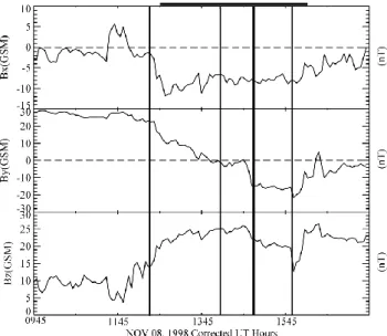
Fig. 8. Shown are magnetic field data from the ACE satellite which orbits the L1 Lagrangian point about 200 REsunward of the Earth. IMF GSM components are plotted for 8 November 1998, as a func-tion of corrected universal time (UT plus the estimated propagafunc-tion time from the satellite to GSM X=0); about 45 min. The thick verti-cal line marks the time when Polar UVI shows a TPA aligned along the noon-midnight meridian in the Northern Hemisphere. The three thin vertical lines mark the time when DMSP F13 reaches highest latitudes over the Northern Hemisphere. The thick horizontal line at the top denotes the time period when UVI data are available.
2.3 Event of 8 November 1998
In Fig. 8 we show magnetic field data from the ACE (Ad-vanced Composition Explorer) spacecraft that orbits the L1 Lagrangian point approximately 200 RE sunward of the Earth. IMF GSM components are plotted for 8 November 1998, as a function of corrected universal time (UT plus the estimated propagation time from the satellite to GSM X=0); in this event the correction is about 45 min. The thick verti-cal line marks the time when POLAR UVI observes a TPA aligned along the noon-midnight meridian in the Northern Hemisphere. The three thin vertical lines mark the time when DMSP F13 reaches highest latitudes over the North-ern Hemisphere. The thick horizontal line at the top denotes the time period when UVI data is available.
IMF Bzis positive for at least 3 h prior to and following a change in By. IMF Bxis negative through the time period of interest. Byis small for 1 to 1.5 h while changing sign. ACE plasma measurements (not shown) indicate that during the time of the IMF Bychange, solar wind ion density is about 20 cm−3and solar wind velocity is approximately 550 km/s. To map the solar wind electric field to the polar ionosphere using the Paraboloid Model, the Dstand AL geomagnetic in-dices are needed. The event studied (see Fig. 9) corresponds to quiet or slightly disturbed time. Dst is about −50 nT and ALis −400, −69, and −93 nT, respectively, for the three in-stants modelled. The model polar cap magnetic flux changed from 740 to 430 MWb during the evolution of the TPA.
Fig. 9. Left: Data shown from three DMSP passes on 8 November 1998 (12:17–12:41, 13:59–14:19, and 15:41–16:01 UT) that occur during the Polar UVI data period. DMSP F13 and F14 horizontal plasma flows, perpendicular to the satellite track, are plotted over a UV image taken at the time when F13 is at highest magnetic lati-tudes. Right: For the same 3 times are shown the modelled polar cap boundary, auroral oval, and polar cap convection generated by the solar wind electric field, as predicted by the Paraboloid Model. The model parameters for each case were calculated from solar wind data and geomagnetic indices. For UT=14:09:48 the TPA observed in the dusk sector may be explained by the time delay (∼20 min) between the IMF turning and the ionospheric convection response (Clauer et al., 2001). At 13:49:48 UT IMF Bywas slightly positive, which corresponds to the observed TPA location. Red curves show the electrostatic potential patterns (10 kV contour separation). See text for details.
POLAR UVI provides images in the Northern Hemi-sphere. In this event the transpolar arc originates on the dusk-side of the auroral oval and migrates across the entire polar region. Around 12:28 UT the duskside of the auroral oval has expanded poleward, as expected for positive Bzand positive By, and has a bright poleward edge. IMF By changes sign from positive to negative at approximately 14:00 UT then decreases approximately 14 nT at 14:45 UT. IMF Bxis neg-ative and Bz remains positive (ranging from 13–26 nT for the next 9 h). During the next hour (14:00 to 15:00 UT) the TPA moves dawnward. At 15:01 UT, approximately 1 h af-ter Bybecomes negative/near zero and approximately 15 min after Bybecomes more strongly negative, the transpolar arc
has moved to highest latitudes and is aligned along the noon-midnight meridian, forming what is commonly referred to as theta aurora. The dawnside of the auroral oval has expanded poleward, as expected for negative By. The arc continues its dusk to dawn motion and by 16:15 UT it has moved across the polar region and appears to be part of the dawnside auro-ral oval.
Figure 9 shows, in the left column, POLAR UV images in the Northern Hemisphere with DMSP F13 and 14 horizontal plasma flows are plotted over each UV image for the three Northern Hemisphere passes available during the TPA evo-lution. The data shown at the top occur during positive By and northward IMF. DMSP F13 shows a spatially expanded duskside region of sunward flow that is bifurcated by a small antisunward flow region. This pattern has three sunward and two antisunward flow regions, producing four convection re-versal boundaries (CRBs), where, for southward IMF, two CRBs are expected. The high-latitude convection pattern is dominated by sunward flow, some of which can be closed in the dawnside antisunward flow region, producing clockwise (negative potential) circulation in a cell located at highest latitudes on the dawnside of the polar region. The sunward flow associated with the TPA may be closed in the antisun-ward flow region equatorantisun-ward, resulting in a local maximum in the negative potential region. In addition to an expanded duskside sunward flow region during positive Bzand By, we expect an expanded duskside auroral oval.
The equipotentials in the polar cap mapped from the mag-netopause using the MSU paraboloid model are shown on the right. The MSU paraboloid model calculates the equa-torward boundary of the auroral oval (thick grey curve), de-fined as the projection of the earthward edge of the magne-tospheric tail current sheet. Also shown are the convection contours obtained by mapping the electric potentials from the magnetopause along open field lines into the ionosphere (negative potential, red curves). There is good agreement be-tween the equatorward boundary of the auroral oval and the UV image. The negative potential dominates the polar re-gion, with a potential difference of 103 kV at high latitudes in the KTH numerical model and 98 kV in the MSU paraboloid model. The model polar cap magnetic flux was calculated using its equality to the tail lobe magnetic flux. The assump-tion E||=0 allows us to calculate the ionospheric electric field from the known distribution of the electric potential at the magnetopause, in turn calculated by the method described by Alexeev et al. (2003).
By the time of the second DMSP pass (middle plot of Fig. 9), IMF By has changed sign from positive to weakly negative. Both DMSP F13 and F14 reach higher magnetic latitudes than in the previous pass. On the dayside large anti-sunward and anti-sunward flows are seen in what is traditionally the polar cap. Previously, the sunward flow was dominated by clockwise circulation (negative potential) in a dawn cell, whereas now it is dominated by counterclockwise circulation (positive potential) in a high-latitude dusk cell. The trans-polar arc has moved to higher latitudes, and is still located on the duskside of the noon-midnight meridian. The arc
re-mains collocated with the duskside of the high-latitude sun-ward flow region, and both are now at higher latitudes than in the previous pass.
To the right, we show the corresponding equipotentials on open field lines projected to the ionospheric level. The po-lar cap potential drop is δ8pc=58 kV. The figure illustrates the location of the convection patterns relative to the noon-midnight meridian and explains the TPA location along it. However, the calculated polar cap size is smaller than the one estimated from POLAR data.
At the time of the observations shown at the bottom of Fig. 9, IMF Bz is still positive and IMF By has been nega-tive (or weakly neganega-tive) for about 2 h. Both DMSP satel-lites have reached higher magnetic latitudes than in the pre-vious orbit, with the F13 satellite track now aligned along the dawn-dusk meridian. The flow pattern has two main CRBs, the one located at highest latitudes is associated with a spa-tially expanded dawnside sunward flow region. The iono-spheric convection pattern is still dominated by a counter-clockwise circulating cell (positive potential) that is located at highest latitudes. The transpolar arc is located on the dawnside of the noon-midnight meridian but is still collo-cated with the duskward edge of the high-latitude sunward flow region.
The bottom right dial shows the polar cap convection at 15:51:04 UT on 8 November 1998, obtained from the Paraboloid Model. In this case the azimuthal component of the IMF, By, was negative and of the order of Bz. The polar cap potential drop of δ8pc=95 kV is larger than that (73 kV) obtained by the KTH model.
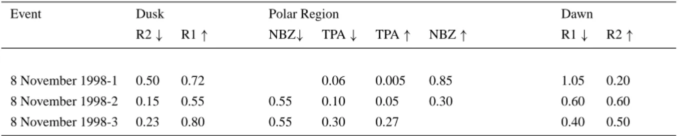
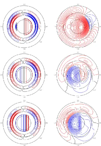
Figure 10 shows on the left model field-aligned current patterns for each of the DMSP passes on 8 November 1998, and on the right the electrostatic potential patterns generated by the KTH model. Upward and downward FACs are shown in red and blue, respectively, positive potentials are shown in blue and negative in red. The black line denotes zero po-tential. In the top left of Fig. 10, the TPA FACs reflect the motion of the TPA, first on the duskside of the auroral re-gion, then at higher latitudes near the noon-midnight merid-ian, then finally the TPA has moved to the dawnside of the noon-midnight meridian. POLAR UVI (not shown) tracks the continued dawnward motion of the TPA. Table 1 lists the model input values for the FACs.
The maximum and minimum values of the electrostatic potentials are shown in Table 2. The last two columns show the values of the polar cap potential drops in the KTH and Paraboloid Models, respectively.
The Paraboloid Model gives the potential drop across the polar cap δ8r as
δ8r=bv1y. (6)
Here b=kbB is the IMF penetrating the magnetosphere, v=kvV is the plasma velocity at the open field line bundle boundary near the magnetopause, and 1y is the width of the open magnetic field line bundle at the magnetopause.
Table 1. Modelled field-aligned current values (MA) for 8 November 1998.
Event Dusk Polar Region Dawn
R2 ↓ R1 ↑ NBZ↓ TPA ↓ TPA ↑ NBZ ↑ R1 ↓ R2 ↑
8 November 1998-1 0.50 0.72 0.06 0.005 0.85 1.05 0.20
8 November 1998-2 0.15 0.55 0.55 0.10 0.05 0.30 0.60 0.60
8 November 1998-3 0.23 0.80 0.55 0.30 0.27 0.40 0.50
Table 2. Local potential extrema (kV) for 8 November 1998.
Event Dusk Noon-midnight Dawn δ8KT H δ8pc−parab Meridian
8 November 1998-1 −45 −90 +13 103 98
8 November 1998-2 −13 +45 −8 +8 58 58
8 November 1998-3 −25 +48 +9 73 95
To calculate δ8pc, the transpolar potential drop, we take into account the saturation effect (Siscoe et al., 2002):
δ8pc=δ8rδ8s/(δ8r+δ8s). (7)
The coefficient kb=0.2 for the magnetic field was determined based on the results of Alexeev et al. (2003). The coefficient
kv was determined as 0.4. The saturation potential value δ8s=158 kV was determined based on Siscoe et al. (2002). Equations (6) and (7) give, for the case of 8 November 1998, 14:09:48 UT (when By=0), a polar cap potential drop of 58 kV, which is in good accordance with the KTH model re-sult ∼58 kV (see Table 2), as well as with the DMSP F13 ion drift observations. These values of the coefficients in Eqs. (6) and (7) correspond to an 8% ratio of the ionospheric transpo-lar potential drop to the potential drop across the open field line bundle in the solar wind. From an analysis of the polar cap potential drop dependent on the IMF, Reiff et al. (1981) estimated this ratio as 10–20%. Kelley et al. (2003) deter-mined the ratio of the dawn-dusk electric field measured by ground-based radars at the equatorial ionosphere to the inter-planetary electric field registered by ACE to be 7%.
2.4 Event of 11 February 1999
In Fig. 11 we show magnetic field data from ACE at L1. IMF GSM components are plotted for 11 February 1999, as a function of corrected universal time; here the correction is about 1 h. The thick vertical line marks the time when Polar UVI shows a TPA aligned along the noon-midnight meridian in the Northern Hemisphere. The three thin ver-tical lines mark the time when DMSP F13 reaches highest latitudes over the Northern Hemisphere. The thick horizon-tal line at the top denotes the time period when UVI data are available.
ACE plasma measurements (not shown) indicate that dur-ing the time of the IMF Bychange, solar wind ion density is about 30 cm−3and solar wind velocity is about 430 km/s.
The event studied (see Fig. 12) corresponds to quiet time.
Dst is 11 nT and AL is 9.2, 34.6, and 21.8 nT, respectively, for the three instants modelled. The model polar cap mag-netic flux is about 420 MWb. Similar to Fig. 9, both auroral oval boundaries and predicted TPA positions are shown.
In this event UVI observed a transpolar arc originating on the dawnside of the auroral oval and subsequently migrat-ing across the entire polar region. Between approximately 19:15 and 20:00 UT (not shown) the dawnside of the auroral oval expands poleward, as expected for negative Byand pos-itive Bz. Between approximately 20:00 and 21:30 UT, Byis weakly positive while changing sign from negative to posi-tive. During this time the TPA appears to begin separating from the dawnside auroral oval and is clearly separated by 20:40 UT. As expected for positive By, the duskward migra-tion of the TPA is accompanied by a poleward expansion of the duskside oval (21:40 UT). In this case an arc forms at the poleward edge of the duskside auroral oval and appears to separate by 22:00 UT. At 22:20 UT the dawnside originat-ing TPA is aligned along the noon-midnight meridian, about 140 min after By becomes positive/near zero and about an hour after Bybecomes more strongly positive. At 22:40 UT the TPA is located just on the duskside of the noon-midnight meridian and is clearly attached to the dayside auroral oval. By 00:45 UT on 12 February 1999 the dawn originating TPA has merged with the duskside oval.
The top plot of Fig. 12 shows data from the first DMSP pass when IMF Bz is northward, IMF By is changing from negative to weakly positive and IMF Bx is changing from positive to negative. DMSP F13 shows a spatially expanded
Fig. 10. Shown on the left, modelled field-aligned current patterns (0.1µA/m2contour separation) for each of the DMSP passes on 8 November 1998; and on the right, the electrostatic potential patterns (3 kV contour separation) generated by the KTH model. Upward and downward FACs are shown in red and blue, respectively; posi-tive potentials are shown in blue and negaposi-tive in red. The black line denotes zero potential. See text for more details.
dawnside region of sunward flow that is bifurcated by small antisunward flow regions. The sunward flow associated with the TPA may be closed in the antisunward flow region equa-torward, resulting in a local minimum in the positive poten-tial region. This pattern is similar to the first pass of the first event (8 November 1998), except that the expansion is from the dawnside, as expected for negative By. The high-latitude convection pattern is dominated by sunward flow, some of which can be closed in the duskside antisunward flow region producing anticlockwise (positive potential) circulation in a cell located at highest latitudes on the duskside of the polar region.
By the time of the second DMSP pass, shown in the middle plot of Fig. 12, IMF Byhas become more strongly positive. DMSP F13 passes at lower latitudes on the dayside than in the previous orbit. Convection is now dominated by clock-wise circulation (negative potential), as expected for positive
By. The TPA appears to have separated from the dawnside auroral oval and a second arc has formed at the poleward edge of the duskside auroral oval co-located with the sun-ward plasma flow.
Fig. 11. Shown are magnetic field data from the ACE satellite which orbits the L1 Lagrange point about 200 RE sunward of the Earth. IMF GSM components are plotted for 11 February 1999, as a func-tion of corrected universal time (UT plus the estimated propagafunc-tion time from the satellite to GSMX=0); about 1 h. The thickest ver-tical line marks the time when the TPA is aligned along the noon-midnight meridian. The thick horizontal line at the top denotes the time period when UVI data are available.
By the last DMSP pass for this event (bottom plot of Fig. 12), IMF Bz is still positive and By has been positive for about 3 h. The dawnside originating TPA has migrated to the duskside and faded. DMSP F13 is located at lower magnetic latitudes than in the previous pass, passing again through the poleward edge of the dayside auroral oval. Spa-tially expanded duskside sunward flow can be closed in a strong antisunward flow region, resulting in a large clock-wise circulating (negative potential) cell dominating the day-side region. The right-hand column in Fig. 12 shows the convection patterns on open field lines projected using the Paraboloid Model.
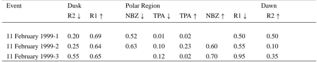
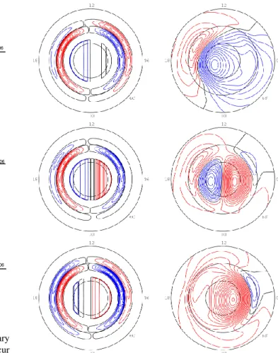
Figure 13 shows, on the left, model field-aligned current distributions for each of the DMSP passes on 11 February 1999, and on the right, the electrostatic potential patterns generated by the KTH model. Upward and downward FACs are shown in red and blue, respectively, and positive poten-tials are shown in blue and negative in red. The black line denotes zero potential. The TPA FACs reflect the dawn to dusk motion of the TPA. Table 3 lists the model input values for the FACs.
The maximum and minimum values of the electrostatic potentials are shown in Table 4. The last column shows the values of the polar cap potential drops in the Paraboloid Model, δ8pc−parab, (see Sect. 2.5).
Table 3. Modelled field-aligned current values (MA) for 11 February 1999.
Event Dusk Polar Region Dawn
R2 ↓ R1 ↑ NBZ ↓ TPA ↓ TPA ↑ NBZ ↑ R1 ↓ R2 ↑
11 February 1999-1 0.20 0.69 0.52 0.01 0.02 0.50 0.50
11 February 1999-2 0.25 0.64 0.63 0.10 0.23 0.60 0.55 0.10
11 February 1999-3 0.55 0.65 0.12 0.02 0.70 0.95 0.35
Table 4. Local potential extrema (kV).
Event Dusk Noon-midnight Dawn δ8KT H δ8pc−parab Meridian
11 February 1999-1 −20 +41 +20 61 74
11 February 1999-2 −17 +29 −53 +5 82 67
11 February 1999-3 −20 −63 +9 72 75
3 Discussion and conclusions
This paper addresses the class of high-latitude aurora that in-volves moving transpolar arcs forming theta aurora as they traverse the highest latitudes. Theta aurorae were first ob-served on a global scale by Frank et al. (1982) from Dy-namics Explorer 1 images. Before that a multitude of lo-calised observations of high-latitude aurora had been made (e.g. Mawson, 1916; Davis, 1960; Denholm, 1961; Denholm and Bond, 1961; Davis, 1963; Eather and Akasofu, 1969; Berkey et al., 1976; Lassen and Danielsen, 1978), but be-cause of the limited field of view of imagers located on the ground or onboard low-altitude spacecraft, the global nature of some of these arcs was not recognised.
Valladares et al. (1994) performed a comprehensive statis-tical study of the occurrence of high-latitude arcs and their dependence on the IMF, based on all-sky images. They also investigated the motion of the arcs and found the same kind of IMF dependence of the direction of motion that has later been established for transpolar arcs (e.g. Cumnock et al., 1997), although many of the arcs in their study belonged to different classes of high-latitude aurora.
Several models have been developed that attempt to ex-plain transpolar arcs (e.g. Chang et al., 1998; Newell et al., 1999; Kullen, 2000; Slinker et al., 2001; Kullen and Jan-hunen, 2004; Naehr and Toffoletto, 2004; and references therein), although none of them producs arcs that reach the dayside oval. Others (e.g. Maynard et al., 2003) ad-dress additional types of auroral arcs at high latitudes dur-ing northward IMF. When trydur-ing to relate the occurrence of high-latitude auroral arcs, the corresponding magnetospheric topology, and the physical mechanisms causing them, to models and simulations, we must carefully consider the do-main of validity of each model. Whereas some features may
be common to the different types of arcs, it is certainly not a valid assumption that all features are common. For exam-ple, Maynard et al. (2003), relate midnight originating Sun-aligned arcs to high-pressure channels in the distant plasma sheet. Whereas their results are certainly interesting in re-lation to midnight originating arcs, their applicability to the class of arcs that we are addressing is not at all clear.
In the spherical model it was shown that when Bychanges sign, the line dividing the two polar convection cells and the corresponding auroral emissions, aligned along the noon-midnight meridian, should drift in either the dawn or dusk di-rection. When Bychanges from negative to positive (positive to negative) it moves from dawn to dusk (from dusk to dawn), in good agreement with our observations and also with ear-lier reports (e.g. Cumnock et al., 1997, 2002; Cumnock and Blomberg, 2004).
In the Paraboloid model, in contrast to the Spherical model, the reconnection efficiency coefficients are differ-ent for the parallel and orthogonal compondiffer-ents of the IMF, and both of them can be calculated self-consistently from the magnetosheath plasma flow solution (see Alexeev et al. (2003) for a thorough explanation). We use both of the magnetospheric models because one of them (the spherical) enables a simple and clear explanation of the TPA mecha-nism, whereas the other one (the paraboloid) gives quantita-tive results for ionospheric plasma convection patterns and auroral oval location that can be compared with the KTH model and satellite observations.
The TPA (associated with closed field lines) originates as part of the dawn or dusk side auroral oval. As it moves to higher latitudes it is surrounded by regions void of ions and filled with polar rain electrons (associated with open field lines). The TPA then continues to move across the polar re-gion and becomes part of the opposite oval from where it
Fig. 12. Left: Data shown from three DMSP passes on 11 February 1999 (19:46–20:06, 21:29–21:49, and 23:10–23:30 UT) that occur during the Polar UVI data period. DMSP F13 horizontal plasma flows, perpendicular to the satellite track are plotted over a UV im-age taken at the time when F13 is at highest magnetic latitudes. Right: For the same 3 times are shown the model calculations of the polar cap boundary, auroral oval, and polar cap convection gen-erated by solar wind electric field, all derived from the Paraboloid Model. The model parameters for each case were calculated from solar wind data and geomagnetic indices. See text for details.
originated. This separation implies a highly distorted and dynamic magnetotail configuration.
Model calculations give us the polar cap electric field po-tential drop as well as the parallel popo-tential difference applied to the separatrices and the acceleration of the auroral parti-cles which creates the TPA. The model results explain the correlation between TPA occurrence and the By component of the IMF because the potential drop on the separatrix, δ8, is proportional to By. They support the observed TPA mo-tion from dawn to dusk or opposite with the change in sign of IMF By. In accordance with observations, the TPA re-gion is collocated with sunward ionospheric convective flow. Additional study is needed to explain why the model gives a smaller polar cap size than the size of the visible dark area in the polar region. It is not yet clear what the magnetospheric field feature is that corresponds to the poleward boundary of the auroral oval. Also, the model does not account for the existence of a TPA when IMF By=0.
Fig. 13. Shown on the left, modelled field-aligned current patterns (0.1µA/m2contour separation) for each of the DMSP passes on 11 February 1999; and on the right, the electrostatic potential patterns (3 kV contour separation) generated by the KTH model. Upward and downward FACs are shown in red and blue, respectively; posi-tive potentials are shown in blue and negaposi-tive in red. The black line denotes zero potential. See text for more details.
We suggest that the auroral emissions in transpolar auroral arcs are caused, on a global scale, by the potential difference that exists between the northern and southern magnetic null points for IMF By6=0. On the local scale, for the potential difference along a particular magnetic field line traversing the transpolar arc the acceleration potential is determined by the electric potential at the ionospheric footpoint of each field line and the fact that all boundary field lines share a common potential at their magnetospheric end. Thus, we should ex-pect auroral emissions at the boundary between the two cells in the open field line regions in the polar caps for northward IMF. The emission region should be associated with reverse convection.
Acknowledgements. The authors thank G. Parks for providing
PO-LAR UVI data, F. Rich for providing the DMSP F13 and F14 SSIES, SSJ4/4 and SSM data, WDC-2 at Kyoto for providing Dst and AL indexes. We thank the ACE MAG and SWEPAM instru-ment teams and the ACE Science Center for providing the ACE data. Work at the Royal Institute of Technology was supported by
the Swedish National Space Board. Work at the University of Texas at Dallas was supported by NSF Grant ATM0211572. Work at the Moscow State University was supported by Russian Basic Research Grants 01-05-65003 and 04-05-64396. The collaboration between the Alfv´en Laboratory and Moscow State University was supported by a grant from the Royal Swedish Academy of Sciences.
Topical Editor T. Pulkkinen thanks three referees for their help in evaluating this paper.
References
Alexeev I. I.: The penetration of interplanetary magnetic and elec-tric fields into the magnetosphere, J. Geomagn. Geoelectr., 38, 1199–1221, 1986.
Alexeev, I. I. and Belenkaya, E. S.: Electric field in an open model of the magnetosphere (in Russian), Geomagn. Aeron., 23, 75–81, 1983.
Alexeev, I. I. and Belenkaya, E. S.: Magnetospheric plasma convec-tion on the open field lines, Geomagn. Aeron. (in Russian), 25, 450–457, 1985.
Alexeev, I. I., Belenkaya, E. S., Bobrovnikov, S. Yu., and Kalegaev, V. V.: Modelling of the electromagnetic field in the interplanetary space and in the Earth’s magnetosphere, Space Sci. Rev., 107, Issue 1–2, 7–26, 2003.
Belenkaya, E. S.: Reconnection modes for near-radial interplan-etary magnetic field, J. Geophys. Res., 103, 26 487–26 494, 1998a.
Belenkaya, E. S.: High-latitude ionospheric convection patterns de-pendent on the variable IMF orientation, J. Atmos. Sol. Terr. Phys., 60, 1343–1354, 1998b.
Belenkaya, E. S.: The IMF influence on the forming of the magne-tosphere, ITOGY NAUKI I TECHNIKI, Issledovanie kosmich-eskogo prostranstva (in Russian), 33a, Moscow, VINITI, 235, 2002.
Berkey, F. T., Cogger, L. L., Ismail, S., and Kamide, Y.: Evidence for a correlation between Sun-aligned arcs and the interplanetary magnetic field direction, Geophys. Res. Lett., 3, 145–147, 1976. Blomberg, L. G. and Cumnock, J. A.: Electrodynamics of transpo-lar aurorae, Adv. Space Res., doi:10.1016/j.asr.2004.06.022, in press, 2005.
Blomberg, L. G. and Marklund, G. T.: High-latitude electrodynam-ics and aurorae during northward IMF, in Auroral Plasma Dy-namics, Geophys. Monogr. Ser., 80, (Ed.) Lysak, R. L., 55–68, AGU, Washington, D. C., 1993.
Blomberg, L. G. and Marklund, G. T.: A numerical model of iono-spheric convection derived from field-aligned currents and the corresponding conductivity, Rep. TRITA-EPP-91-03, 29, Royal Inst. of Technology, Stockholm, 1991a.
Blomberg, L. G. and Marklund, G. T.: High-latitude convection pat-terns for various large-scale field-aligned current configurations, Geophys. Res. Lett., 18, 717–720, 1991b.
Carlson, H. C., Heelis, R. A., Weber, E. J., and Sharber, J. R.: Coherent mesoscale convection patterns during northward inter-planetary magnetic field, J. Geophys. Res., 93, 14 501–14 514, 1988.
Chang, S.-W., Scudder, J. D., and Sigwarth, J. B. et al.: A compari-son of a model for the theta aurora with observations from Polar, Wind, and SuperDARN, J. Geophys. Res., 103, 17 367–17 390, 1998.
Clauer, C. R. Jr., Alexeev, I. I., Belenkaya, E. S., and Baker, J. B.: Special features of the 24–27 September 1998 storm during
high solar wind dynamic pressure and northward interplanetary magnetic field, J. Geophys. Res., 106, 25 695–25 712, 2001. Cowley, S. W. H.: A qualitative study of the reconnection between
the Earth’s magnetic field and an interplanetary field of arbitrary orientation, Radio Sci., 8, 903–913, 1973.
Cumnock, J. A.: High-latitude aurora during steady northward in-terplanetary magnetic field and changing IMF By, J. Geophys. Res., A02304, 110, doi:10.1029/2004JA010867, 2005.
Cumnock, J. A. and Blomberg, L. G.: Transpolar arc evolution and associated potential patterns, Ann. Geophys., 22, 1213–1231, 2004,
SRef-ID: 1432-0576/ag/2004-22-1213.
Cumnock, J. A., Heelis, R. A., Hairston, M. R., and Newell, P. T.: High-latitude ionospheric convection pattern during steady northward interplanetary magnetic field, J. Geophys. Res., 100, 14 537–14 554, 1995.
Cumnock, J. A., Sharber, J. R., Hairston, M. R., Heelis R. A., and Craven, J. D.: Evolution of the global auroral pattern during pos-itive IMF Bz and varying IMF By conditions, J. Geophys. Res., 102, 17 489–17 498, 1997.
Cumnock J. A., Sharber, J. R., Heelis, R. A, Blomberg, L. G., Ger-many, G. A., Spann, J. F., and Coley, W. R.: Interplanetary mag-netic field control of theta aurora development, J. Geophys. Res., 107, doi:10.1029/2001JA009126, 10, 2002.
Davis, T. N.: The morphology of the polar aurora, J. Geophys. Res., 65, 3497–3500, 1960.
Davis, T. N.: Negative correlation between polar cap visual activity and magnetic activity, J. Geophys. Res., 68, 4447–4453, 1963. Denholm, J. V.: Some auroral observations inside the southern
au-roral zone, J. Geophys. Res., 66, 2105–2111, 1961.
Denholm, J. V. and Bond, F. R.: Orientation of polar auroras, Aust. J. Phys., 14, 193–195, 1961.
Eather, R. H. and Akasofu, S.-I.: Characteristics of polar cap auro-ras, J. Geophys. Res., 74, 4794–4798, 1969.
Frank, L. A., Craven, J. D., Burch, J. L., and Winningham, J. D.: Polar views of the Earth’s aurora with Dynamics Explorer, Geo-phys. Res. Lett., 9, 1001–1004, 1982.
Frank, L. A., Craven, J. D., and Gurnett, D. A., et al.: The theta aurora, J. Geophys. Res., 91, 3177–3224, 1986.
Greene, J. M.: Geometrical properties of three-dimensional recon-necting magnetic fields with nulls, J. Geophys. Res., 93, 8583– 8590, 1988.
Gusev, M. G. and Troshichev, O. A.: Relation of sun-aligned arcs to polar cap convection and magnetic disturbances, Planet. Space Sci., 38, 1–11, 1990.
Gussenhoven, M. S.: Extremely high latitude auroras, J. Geophys. Res., 87, 2401–2412, 1982.
Heelis, R. A., Reiff, P. H., Winningham, J. D., and Hanson, W. B.: Ionospheric convection signatures observed by DE 2 during northward interplanetary magnetic field, J. Geophys. Res., 91, 5817–5830, 1986.
Heppner, J. P. and Maynard, N. C.: Empirical high-latitude electric field models, J. Geophys. Res., 92, 4467–4489, 1987.
Hoffman, R. A., Heelis, R. A., and Prasad, J. A.: A sun-aligned arc observed by DMSP and AE-C, J. Geophys. Res., 90, 9697–9710, 1985.
Ismail, S. and Meng, C.-I.: A classification of polar cap auroral arcs, Planet. Space Sci., 30, 319–330, 1982.
Jankowska, K., Elphinstone, R. D,. Murphree, J. S., Cogger, L. L., and Hearn, D.: The configuration of the auroral distribution for interplanetary magnetic field Bz northward, 2. Ionospheric con-vection consistent with Viking observations, J. Geophys. Res.,
95, 5805–5816, 1990.
Kalegaev, V.: Magnetosheath conditions and magnetopause struc-ture for high magnetic shear, Phys. Chem. Earth, 25, 173–176, 2000.
Kelley, M. C., Makela, J. J., Chau, J. L., and Nicolls, M. J: Penetration of the solar wind electric field into the magnetosphere/ionosphere system, Geophys. Res. Lett., 30, doi:10.1029/2002GL016321, 2003.
Kullen, A.: The connection between transpolar arcs and magneto-tail rotation, Geophys. Res. Lett., 27, 73–76, 2000.
Kullen, A. and Janhunen, P.: Relation of polar auroral arcs to mag-netotail twisting and IMF rotation: A systematic MHD simula-tion study, Ann. Geophys., 22, 951–970, 2004,
SRef-ID: 1432-0576/ag/2004-22-951.
Kullen, A., Brittnacher, M., Cumnock, J. A., and Blomberg, L. G.: Solar wind dependence of the occurrence and motion of polar au-roral arcs: A statistical study, J. Geophys. Res., 107(AX), 1362, doi:10.1029/ 2002JA009245, 23, 2002.
Lassen, K. and Danielsen, C.:Quiet-time pattern of auroral arcs for different directions of the interplanetary magnetic field in the Y-Z plane, J. Geophys. Res. 83, 5277–5284, 1978.
Marklund, G. T., Blomberg, L. G., Murphree, J. S., Elphinstone, R. D., Zanetti, L. J., Erlandson, R. E., Sandahl, I., de la Beau-jardi`ere, O., Opgenoorth, H., and Rich, F. J.: On the electrody-namical state of the auroral ionosphere during northward IMF: A transpolar arc case study, J. Geophys. Res., 96, 9567–9578, 1991.
Mawson, D.: Auroral observations at the Cape Royds Station, Antarctica, Trans. Royal Soc. S. Aust., XL, 151–212, 1916. Maynard, N. C., Burke, W. J., and Moen, J., et al.: Responses of
the open closed field-line boundary in the evening sector to IMF changes: A source mechanism for Sun-aligned arcs, J. Geophys. Res., 108(A01006), doi:10.1029/2001JA000174, 2003. Meng, C.-I.: Polar cap arcs and the plasma sheet, Geophys. Res.
Lett., 8, 273–276, 1981.
Menietti, J. D. and Burch, J. L.: DE 1 observations of theta aurora plasma source regions and Birkeland current charge carriers, J. Geophys. Res., 92, 7503–7518, 1987.
Murphree, J. S., Cogger, L. L., Anger, C. D., Wallis, D. D., and Shepherd, G. G.: Oval intensifications associated with polar arcs, Geophys. Res. Lett., 14, 403–406, 1987.
Naehr, S. M. and Toffoletto, F. R.: Quantitative modeling of the magnetic field configuration associated with the theta aurora, J. Geophys. Res., 109( A07202), doi:10.1029/2003JA010191, 2004.
Newell, P. T., Liou, K., Meng, C.-I., Brittnacher, M. J., and Parks, G.: Dynamics of double-theta aurora: Polar UVI study of 10–11 January 1997, J. Geophys. Res., 104, 95–104, 1999.
Obara, T., Mukai, T., Hayakawa, H., Nishida, A., Tsuruda, K., and Fukunishi, H.: Akebono (EXOS D) observations of small-scale electromagnetic signatures relating to polar cap precipitation, J. Geophys. Res., 98, 11 153–11 159, 1993.
Potemra, T. A., Zanetti, L. J., Bythrow, P. F., Lui, A. T. Y., and Iijima, T.: By-dependent convection patterns during northward interplanetary magnetic field, J. Geophys. Res., 89, 9753–9760, 1984.
Reiff, P. H., Spiro, R. W., and Hill, T. W.: Dependence of polar cap potential drop on interplanetary parameters, J. Geophys. Res., 86, 7639–7648, 1981.
Reiff, P. H. and Burch, J. L.: IMF By-dependent plasma flow and Birkeland currents in the dayside magnetosphere, 2, A global model for northward and southward IMF, J. Geophys. Res., 90, 1595–1609, 1985.
Rich, F. J.: Technical description for the topside ionospheric plasma monitor (SSIES, SSIES-2 and SSIES-3) on spacecraft of the De-fense Meteorological Satellite Program (DMSP), Tech. Rep. PL-TR-94-2187, 69, Air Force Phillips Lab., Bedford, Mass., 1994. Robinson, R. M. and Mende, S. B.: Ionization and electric field
properties of auroral arcs during magnetic quiescence, J. Geo-phys. Res., 95, 21 111–21 121, 1990.
Siscoe, G. L., Erickson, G. M., Sonnerup, B. U. ¨O., Maynard, N. C., Siebert, K. D., Weimer, D. R., and White, W. W.: Global role of Ekin magnetopause reconnection: An explicit demonstration, J. Geophys. Res., 106, 13 015–13 022, 2001.
Siscoe, G. L., Erickson, G. M., Sonnerup, B. U. ¨O., Maynard, N. C., Schoendorf, J. A., Siebert, K. D., Weimer, D. R., White, W. W., and Wilson, G. R.: Hill model of transpolar potential satu-ration: Comparisons with MHD simulations, J. Geophys. Res., 107, doi:10.1029/2001JA000109, 2002.
Slinker, S. P., Fedder, J. A., McEwen, D. J., Zhang, Y., and Lyon, J. G.: Polar cap study during northward interplanetary magnetic field on 19 January 1998, Phys. Plasmas, 8, 1119–1126, 2001. Toffoletto, F. R. and Hill, T. W.: Mapping of the solar wind electric
field to the Earth’s polar cap, J. Geophys. Res., 94, 329–347, 1989.
Torr, M. R., Torr, D. G., Zukic, M., Johnson, R. B., Ajello, J., Banks, P., Clark, K., Cole, K., Keffer, C., Parks, G., Tsurutani, B., and Spann, J.: A far ultraviolet imager for the international solar-terrestrial physics mission, Space Sci. Rev., 71, 329–383, 1995.
Valladares, C. E., Carlson, H. C., and Fukui, K.: Interplanetary magnetic field dependency of stable Sun-aligned polar cap arcs, J. Geophys. Res., 99, 6247–6272, 1994.
Zanetti, L. J., Potemra, T. A., Erlandson, R. E., Bythrow, P. F., An-derson, B. J., Murphree, J. S., and Marklund, G. T.: Polar re-gions Birkeland currents, convection and aurora for northward interplanetary magnetic field, J. Geophys. Res., 95, 5825–5833, 1990.