HAL Id: hal-00317086
https://hal.archives-ouvertes.fr/hal-00317086
Submitted on 1 Jan 2002
HAL is a multi-disciplinary open access
archive for the deposit and dissemination of
sci-entific research documents, whether they are
pub-lished or not. The documents may come from
teaching and research institutions in France or
abroad, or from public or private research centers.
L’archive ouverte pluridisciplinaire HAL, est
destinée au dépôt et à la diffusion de documents
scientifiques de niveau recherche, publiés ou non,
émanant des établissements d’enseignement et de
recherche français ou étrangers, des laboratoires
publics ou privés.
OVATION: Oval variation, assessment, tracking,
intensity, and online nowcasting
P. T. Newell, T. Sotirelis, J. M. Ruohoniemi, J. F. Carbary, K. Liou, J. P.
Skura, C.-I. Meng, C. Deehr, D. Wilkinson, F. J. Rich
To cite this version:
P. T. Newell, T. Sotirelis, J. M. Ruohoniemi, J. F. Carbary, K. Liou, et al.. OVATION: Oval variation,
assessment, tracking, intensity, and online nowcasting. Annales Geophysicae, European Geosciences
Union, 2002, 20 (7), pp.1039-1047. �hal-00317086�
Annales
Geophysicae
OVATION: Oval variation, assessment, tracking, intensity, and
online nowcasting
P. T. Newell1, T. Sotirelis1, J. M. Ruohoniemi1, J. F. Carbary1, K. Liou1, J. P. Skura1, C.-I. Meng1, C. Deehr2, D. Wilkinson2, and F. J. Rich3
1The Johns Hopkins University Applied Physics Laboratory Laurel, Maryland, 20723, USA 2University of Alaska at Fairbanks, Fairbanks, Alaska, USA
3Air Force Research Laboratory Hanscom AFB, Massachusetts, USA
Received: 1 October 2001 – Revised: 26 February 2002 – Accepted: 12 March 2002
Abstract. The location of the auroral oval and the
inten-sity of the auroral precipitation within it are basic elements in any adequate characterization of the state of the magneto-sphere. Yet despite the many ground-based and spacecraft-borne instruments monitoring various aspects of auroral be-havior, there are no clear and consistent answers available to those wishing to locate the auroral oval or to quantify its in-tensity. The purpose of OVATION is to create a tool which does so. OVATION is useful both for archival purposes and for space weather nowcasting. The long-running DMSP par-ticle data set, which covers both hemispheres, and has oper-ated since the early 1980s, and which will continue to operate well into the next decade, is chosen as a calibration standard. Other data sets, including global images from Polar UVI, SuperDARN boundaries, and meridian scanning photometer images, are cross-calibrated to the DMSP standard. Each in-corporated instrument has its average offset from the DMSP standard determined as a function of MLT, along with the standard deviations. The various data can, therefore, be com-bined in a meaningful manner, with the weight attached to a given boundary measurement varying inversely with the vari-ance (square of the standard deviation). OVATION currently spans from December 1983 through the present, including real-time data. Participation of additional experimenters is highly welcomed. The only prerequisites are a willingness to conduct the prescribed cross-calibration procedure, and to make the data available online. The real-time auroral oval lo-cation can be found here: http://sd-www.jhuapl.edu/Aurora/ ovation live/north display.html.
Key words. Magnetospheric physics (auroral phenomena;
energetic particles, precipitating; magnetosphere – iono-sphere interactions)
Correspondence to: P. T. Newell
1 Introduction
The auroral oval is the symbolic center of space weather re-search. Space weather as a discipline can be traced back several centuries to early observations of the aurora (Eather, 1980; Schr¨oder, 1984). In a geophysical sense as well, the auroral oval is central. The convergence of the Earth’s ge-omagnetic field means that most of the magnetosphere is tightly coupled to the auroral oval. The aurora can even be used to define the state of the magnetosphere: for example, the most widely accepted definition of a substorm involves auroral behavior.
Yet the most basic questions about the aurora cannot be re-liably or consistently answered, either on a historical basis, or for nowcasting purposes. These questions are: (1) Where is the auroral oval? and (2) How intense is the aurora? The pur-pose of the OVATION project is to provide a tool to the scien-tific community and general public alike which answers these questions in a consistent manner over many decades. OVA-TION is intended as a multi-institutional effort open to all, incorporating a variety of data sources. Currently, scientists at the Johns Hopkins University Applied Physics Laboratory, the University of Alaska at Fairbanks, and the Air Force Re-search Laboratory at Hanscom AFB are all involved. The current version of OVATION includes SuperDARN HF radar data, DMSP particle data, UAF MSP images, and Polar UVI images. We hope many others will join the effort to establish an international standard for determining the position and in-tensity of the auroral oval.
2 Calibration standard: defining the boundaries of the auroral oval
2.1 The choice of standards
To combine data usefully from a diverse set of instruments, it is necessary to have a calibration standard. OVATION uses
1040 P. T. Newell et al.: Oval variation, assessment, tracking, intensity, and online nowcasting the automated boundary routines developed at JHU/APL
(Newell et al., 1991; 1996) and applied to the DMSP SSJ4 particle detectors as that standard. The DMSP satellites pro-vide the worst temporal resolution (about one oval cross-ing per satellite every 25 min) of any technique thus far in-corporated, while also lacking the hemispheric or at least wide-ranging spatial coverage of certain other techniques. Nonetheless, there are several reasons why the DMSP par-ticle data base provides an excellent cross-calibration stan-dard.
First, the continuity of the data set is a major recom-mendation. Nearly two decades of identically instrumented DMSP data is already available (from late 1983 through the present), with a high probability of many more years to come (DMSP may be replaced by 2010, but the replacement satel-lites will likely include a similar auroral energy particle de-tector). Such continuity is a highly desirable attribute for a proposed standard, and one not achievable with any NASA satellite or satellite program, past or planned.
The SSJ4 and SSJ5 particle detectors are, of course, specifically designed to measure auroral particles, both di-rectly and in situ. They measure electrons and ions at 19 distinct energy levels, ranging from 32 eV to 30 keV. No re-mote sensing technique can infer nearly the same detail of spectral information. The spatial resolution, about 7 km, is adequate for most purposes, and is about a factor of 10 better than that which global UV images have hitherto provided. Of course DMSP satellite particle observations are available in both hemispheres, in summer and winter, and in direct sun-light and in darkness. Indeed, they are essentially indifferent to these considerations. The sensitivity, a few hundredths of an erg/cm2s, is about 1.5 orders of magnitude better than that from global imagers. Altogether, a more ideal calibra-tion standard would not be easy to develop.
Nonetheless, other techniques are much better for the rou-tine monitoring of the aurora. Most of the auroral oval po-sition data in the OVATION data base actually comes from Polar UVI and SuperDARN. The slow, laborious compila-tion of boundary posicompila-tions from DMSP cannot realistically compete with the frequent multi-point measurements avail-able from other means. The SuperDARN data also has the advantage of near real-time availability (as does the Univer-sity of Alaska’s Meridian Scanning Photometer).
The obvious choice for the poleward boundary is the open/closed boundary, as best it can be determined. Sec-tion 2.2 will discuss this issue in greater detail. The most appropriate choice for an equatorward boundary is more am-biguous. Feldstein and Galperin (1985) have vigorously argued that the equatorward boundary of the auroral oval should be considered as the location of the most equator-ward discrete arc (or at least, the earthequator-ward extent of the main plasma sheet, which is b2e or b2i for electrons or ions, re-spectively, in the terminology of Newell et al. (1996). How-ever, a substantial body of work exists using a different equa-torward boundary identified from DMSP, namely the low en-ergy electron boundary (Gussenhoven et al., 1981; Hardy et al., 1981). This boundary has been used successfully in many
research papers (e.g. Gussenhoven et al., 1983). The low-energy electron equatorward boundary has also been used by the Air Force for space weather forecasting for years, and has been found useful by HF (“short-wave”) radio operators. Finally, the low-energy electron boundary has a clear geo-physical meaning, both theoretically and experimentally, cor-responding to the zero-energy Alfv´en layer and the plasma-pause (Horwitz et al., 1986).
Therefore we have opted to continue the use of the low-energy electron boundary (which is called b1e in the notation of Newell et al., 1996). The chief drawback to this decision is that many other instrumental techniques are not sensitive enough to directly determine the b1e boundary, and, there-fore, have to rely on statistically determined offsets. Energy fluxes at the b1e boundary are often below 0.1 ergs/cm2s. 2.2 Some algorithmic considerations on the boundaries
de-fined by OVATION
The simple or conceptual explanation for the boundaries used by OVATION was given above, namely the poleward boundary is the open/closed boundary, while the equatorward boundary is the zero-energy electron boundary. In practice, such simple rules do not work without exceptions and modi-fications.
The boundary identification algorithms described by Newell et al. (1996) are used for the nightside boundary iden-tification. Some post processing checks are performed in or-der to discard possible algorithm/code failures. The most common failure is associated with intense penetrating radi-ation, combined with weak auroral oval fluxes, making it occasionally quite difficult to computationally separate the signal from the noise. Data gaps larger than a few seconds in duration, as well as certain other occurrences also result in the discarding of an auroral oval pass. Since a “pass” is defined as extending from the lowest magnetic latitude to the highest magnetic latitude reached, some DMSP passes are discarded simply because the satellite did not reach a lati-tude of at least 1◦poleward of the auroral oval (i.e. reached
into an empty polar cap). It is likely that some of these limi-tations, and others of a similar nature, can be removed in the future with further refinements.
On the nightside, the b6 boundary, the poleward edge of the subvisual drizzle, is used to estimate the open-closed boundary. For the “normal” equatorward boundary, which is
b1e, the zero energy electron boundary is usually used. How-ever, at times, b2i, which represents the peak of the 3–30 keV ion energy flux and a measure of the start of the main plasma sheet, is equatorward of b1e. In this case b2i is used. Most of these exceptional cases occur in the dusk-to-midnight sector. Dayside precipitation regions are identified using the rules outlined in Sect. 4 of Newell et al. (1991). This region in-formation is then parsed, in order to locate the poleward and equatorward boundaries. Specifically, the equatorward boundary is considered located if an unambiguous transition from void (at lower latitudes) to either CPS or BPS (at ad-joining higher latitudes) is observed. The poleward or
open-Fig. 1. The cross-calibration between the DMSP determination of the open-closed boundary and the SuperDARN determination of the CRB. The CRB al-ways lies poleward of the open/closed boundary.
closed boundary is also considered located if an unambigu-ous transition from a closed region (at lower latitudes) to an open region (at higher latitudes) is observed, where CPS and BPS are considered closed, and cusp, mantle, polar rain, and void (at latitudes above the auroral oval) are considered open. The low-latitude boundary layer (LLBL) is classified by the automated identification algorithms as either “open” or “closed”, depending on its spectral characteristics.
Transitions are sometimes considered ambiguous if the spectral characteristics oscillate, or if an apparently incon-sistent transition is observed. (An example of an inconsis-tent transition is from LLBL to BPS, while moving to higher latitudes. Such a transition does not always imply an algo-rithmic error, since the local time might be changing rapidly. It is, however, difficult to interpret clearly.) Such ambiguous poleward boundaries are also discarded from the OVATION data set of DMSP boundaries.
2.3 Cross-calibration
Different boundary sources are calibrated against the DMSP standard using a simple statistical comparison. For data source, s, providing the equatorward and poleward auroral boundaries, beqsand bps, a comparison is made with the
re-spective DMSP boundaries, beq and bp. The average
differ-ences < beqs−beq >and < bps−bp >are calculated as
functions of MLT in order to provide offsets, which compen-sate for differences in the sensitivity of various techniques. Variances are also calculated as a function of MLT, ideally at intervals of 3 h MLT (if the density of data permits):
σeqs2 =(1/n)6i(beqs−beq)2 σps2 =(1/n)6i(bps−bp)2.
When boundary locations from different sources are com-bined, each data set is weighted by the inverse of the appro-priate variance 1/σ2. The exception is the DMSP boundaries, where the weighting functions are based on the time lapsed
1042 P. T. Newell et al.: Oval variation, assessment, tracking, intensity, and online nowcasting
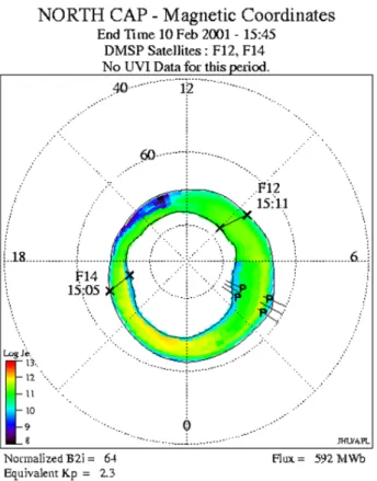
Plate 1: Example of an OVATION display with DMSP data and Polar UVI data. The DMSP boundaries are marked with an “x”, while the Polar UVI boundaries are marked with an “U”. The total integrated polar cap flux is in megawebers. The equivalent instan-taneous Kpis calculated from a linear fit to b2i data.
since the measurement. The average and maximal speed of the auroral oval, determined by comparing two DMSP satel-lites crossing the same location (local time) at differing uni-versal times, is 0.1◦/min and 0.2◦/min (Sotirelis et al., 1998),
which can then be used to define an appropriate variance for the DMSP boundary determinations.
Figure 1 illustrates this approach in practice. We cali-brated SuperDARN determinations of the convection rever-sal boundary (CRB) against the DMSP determination of the open/closed boundary, in 3-h wide local time bins. (No calibration exists between postmidnight and dawn, because DMSP does not often sample this MLT range in the North-ern Hemisphere). As Fig. 1 shows, the CRB lies typically about 1◦ equatorward of the CRB, except at postnoon and at midnight, where the CRB and open/closed boundary are much closer latitudinally. The standard deviation between the SuperDARN CRB and the DMSP poleward boundary is typically 1–2◦. Some of that scatter may be geophysical, but probably a significant portion of the scatter is due to instru-mental and algorithmic “noise”.
One quite fascinating aspect of the cross-calibrations was the discovery that SuperDARN actually calibrates better with the DMSP auroral boundaries than does either Polar UVI or the UAF MSP. For example, the standard deviations between
Plate 2: An example of an OVATION display, combining DMSP boundaries, marked with an “x”, and UAF MSP data, marked with a “P”.
the Polar UVI poleward boundary and the DMSP-determined poleward boundary (not shown) lie between 2.5◦ and 3.5◦. This is just about double the standard deviations from Super-DARN. Of course, the wobble in the Polar spacecraft despun platform may account for a fair fraction of this amount.
3 Integration
3.1 Technical approach
The auroral zone at any particular time is given by deforming an appropriately chosen average boundary shape into agree-ment with observed boundary determinations. This provides some degree of realism in local time sectors where there may not be any observations. The average poleward and equator-ward boundary shapes are taken from Sotirelis and Newell (2000). They are selected according to the current level of magnetotail stretching estimated by the b2i boundary or other surrogate (Sergeev et al., 1993; Newell et al., 1998).
The approach for combining auroral boundary observa-tions is still being improved as the algorithm evolves and better statistical comparisons become available. The statisti-cal weights assigned to the boundary observations are taken from the analysis detailed above and are then decreased ac-cording to their separation in time from the time of interest, using the average open-closed boundary motion of Sotirelis
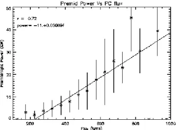
Fig. 2. Correlation of polar cap flux with premidnight auroral power. Bins with no data are plotted as zeros but not included in the fit (which is to the original sample population).
et al. (1998). Due to the low time resolution of the DMSP observations compared to all others in the data base, usu-ally it is only the DMSP boundaries that are impacted by this loss in weighting with elapsed time. Boundary observations in the same MLT hour interval are averaged together using the reciprocal variance as weights. Boundary points are then separated into categories by statistical weight. A point has a high weight if σ ≤ 1.9◦for a single observation or σ ≤ 2.5◦ for an averaged point; otherwise, it is considered to be a low weight.
There is a third category of boundary points available for some instruments. Limit points indicate that a particular boundary is higher or lower in latitude than the indicated po-sition. As of this writing, the only limit points are provided by the SuperDARN radar. In particular, when the equator-ward boundary point (indicated by the sudden onset of scat-ter, and v > 100 m/s) lies almost on top of the radar position, then the actual boundary can easily lie further equatorward. Additionally, the radar measurements can fail in the dawn to noon sector, where very weak electron precipitation can fall over a sizable interval of magnetic latitude, but fail to perturb the ionosphere enough to generate appreciable radar echoes. The initial boundary shape is specified by the magneto-tail stretching index, b2i. The boundary is then deformed to agree exactly (if possible) with all high weight observations, using a scaling factor that varies linearly with MLT (having discontinuous slope at each high weight point). The bound-ary is then further deformed locally (within 3 h) to satisfy any limit points. Lastly, low weight observations are aver-aged with the resulting shape, each deforming the boundary only over a 3-h MLT range.
3.2 Examples
We present two examples of the standard OVATION display. The first, shown in Plate 1, combines a Polar UVI image with
DMSP particle boundaries, to determine the auroral oval po-sition. DMSP boundaries are marked with an “x”, and the UT of each oval crossing by a DMSP satellite appears on the plot. UVI-determined boundaries are marked with a “U”. OVA-TION plots can be viewed in either geographical or geomag-netic coordinates, and with the oval drawn either as a sim-ple monochromatic circle, or with the Sotirelis and Newell (2000) model precipitation intensities. The total magnetic flux within the poleward boundary is calculated and reported in megaWebers (MWb) at the bottom right. The b2i bound-ary measured is normalized to midnight, and is reported also as an equivalent Kp.
Plate 2 presents the second example of an OVATION plot. In this instance, DMSP data is combined with the University of Alaska’s at Fairbanks meridian scanning photometer. As before, the DMSP boundaries are marked with an “x”, while the photometer boundaries are marked with a “P”. Of course, photometer data is available only for a few hours each day, when sunlight, cloud cover, and other conditions permit. The photometer data is available quasi-real time, however.
4 Validation of geophysical usefulness
The most satisfactory way to verify the usefulness of mea-surements, such as that which OVATION provides, is to correlate its outputs – notably 8PC and b2i, the polar cap
flux and magnetotail stretching index – with other geophys-ical phenomena. The usefulness of the magnetotail stretch-ing index, b2i, has been discussed elsewhere (Newell et al., 1998; cf. Sergeev et al., 1983, 1993). Here we concentrate on the magnetospheric state variable, 8PC, which measures
the amount of open geomagnetic flux threading the mag-netotail lobes. Although both of these variables reflect the global magnetic field configuration of the magnetosphere, they are complementary rather than redundant. An analog is the source model of the magnetotail current, in which the intensity of the cross tail current and its distance from Earth are independent parameters (Schulz and McNab, 1987). 4.1 8PCand global auroral power
It turns out that 8PC is highly correlated with total
auro-ral power. In this section and the next, 8PC is calculated
from DMSP measurements alone, while global auroral power is calculated completely independently from Polar UVI im-ages. The DMSP oval positions were all a minimum of three-point fits (thus requiring at least two satellites), with a time resolution of 60 min. Higher time resolution measurements would involve using data sources that were first calibrated to the DMSP standard.
Figure 2 shows the results of correlating polar cap flux (from DMSP boundaries) with premidnight auroral power (from the UVI imager). The correlation is fairly good, namely r = 0.72. (Points along the y = 0 axis in Fig. 2 represent instances of no data within a bin. Since all corre-lations reported are with the original sample population, and
1044 P. T. Newell et al.: Oval variation, assessment, tracking, intensity, and online nowcasting
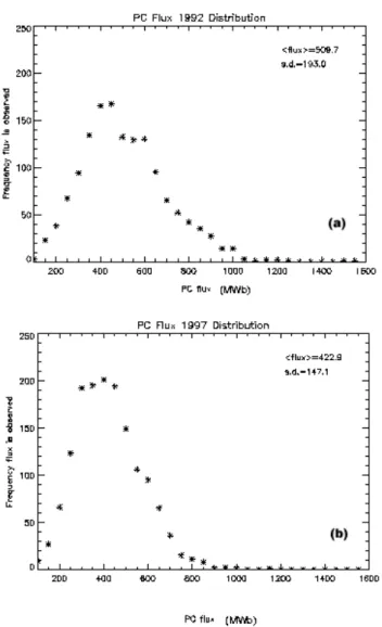
Fig. 3. Distributions of polar cap flux, 8c, for (a) 1992 (an active year) and (b) 1997 (a quiet year). Notice the asymmetry, with a clear large-polar cap size tail.
not with the averages, the cases without data are not included in the fits.) Notice that at higher values of 8PC, auroral power
consistently exceeds the linear fit shown on the figure. In fact, we confirmed that the correlation is actually better be-tween 82PC and auroral power than is a linear fit with 8PC.
Specifically, a fit to the polar cap flux squared improves the correlation coefficient to r = 0.74. In this latter case, how-ever, observed auroral power for the highest values of polar cap flux actually lies below the correlation fit line.
The reason for the nonlinearity is not clear. Some specula-tion that the energy released in a substorm is proporspecula-tional to the polar cap area squared does exist in the literature (Lewis, 1993), but it could hardly be said to have been demonstrated. Total auroral power output probably is directly correlated with total magnetic energy stored in the magnetotail, namely
∼B2TAT, but it is not obvious how this latter quantity relates
to ionospheric observations.
The magnetic energy associated with the open polar cap area (Aion) at ionospheric levels is straightforward, namely
B2ionAion = Bion8PC. This does not necessarily predict the
energy in the magnetotail. The magnetic flux, 8, which is BionAion, is constant between the ionosphere and
magneto-tail. Alas, B2A is not.
Perhaps the nonlinearity is a numerical accident, but the same surplus of auroral power above the linear fit at high val-ues of 8PCis observed at postmidnight as well (not shown).
4.2 Solar cycle variation of 8PC
It is desirable to have some idea of how 8PCvaries over the
course of a solar cycle. Of interest is how the distribution of 8PCduring a geomagnetically active year differs from the 8PC distribution during a quiet year. Although there have
been a few studies about oval boundary motion at given local times, we believe that these results are the first to report the statistical distribution of polar cap flux. Therefore, the results should be of inherent interest.
Figure 3 presents 8PC distributions for 1992 (an active
year) and for 1997 (a comparatively quiet year). Polar cap size does not have a normal distribution; rather it evinces a pronounced skew, with a much more gradual drop off at high polar cap fluxes (active times) than for small polar cap sizes. It is comparatively rare to observe a polar cap flux below 300 MWb, which is only modestly below the mode (most common) value. By contrast, polar cap fluxes 50% greater than the mode were still fairly common in 1992 (the active year). The reason for this asymmetry is that the polar cap only loses open magnetic flux slowly during quiet times; hence it rarely drops to very low values (Newell et al., 1997). At very small polar cap flux levels (below, say, 100 MWb), there is typically a difficulty in accurately measuring the size from DMSP measurements. For example, it requires the DMSP satellites to reach high magnetic latitudes, which is not always the case.
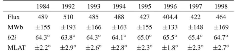
Table 1 lists the mean polar cap flux for a number of years. A reassuring pattern is evident. The polar cap size aver-ages larger during active years (such as 1992) and is smaller during quiet years (such as 1996). Indeed, the better es-tablished and completely independent magnetotail stretch-ing index (b2i) tracks the polar cap flux closely over many years. The pattern shown in polar cap size also agrees with the well-known fact that magnetospheric disturbances peak about 2 years after solar cycle maximum. Hence, it is quite reasonable that the polar cap was the largest in 1992.
Although DMSP is still the best tool within OVATION for solar cycle studies, other data sets provide it with a greater quantity of boundaries, which are more suitable for seasonal and especially for diurnal variation studies, as is discussed in the next section.
4.3 Seasonal and diurnal variations in 8PC
Our final example of how OVATION can be used as a re-search tool concerns the seasonal and diurnal variations in magnetospheric activity. Traditionally, the only means of investigating quantitatively this phenomenon has been by
Table 1. Yearly average values for polar cap flux and magnetotail stretching index. Larger polar cap fluxes and lower latitudes for b2i both indicate more active years
1984 1992 1993 1994 1995 1996 1997 1998
Flux 489 510 485 488 427 404.4 422 464
MWb ±155 ±193 ±166 ±163 ±155 ±133 ±148 ±169
b2i 64.3◦ 63.8◦ 64.3◦ 64.1◦ 65.0◦ 65.5◦ 65.4◦ 64.7◦ MLAT ±2.2◦ ±2.9◦ ±2.6◦ ±2.8◦ ±2.3◦ ±1.8◦ ±2.3◦ ±2.7◦
Plate 3: The seasonal and diurnal variations of the polar cap flux from 1997–1999, as determined by Polar UVI (which contributes the majority of the boundaries in OVATION for those years). The polar cap is largest around equinoxes.
means of indices derived from chains of magnetometer sta-tions. Many valuable results have been learned in this man-ner (Cliver et al., 2000; Lyatsky et al., 2001). Still, it is certainly desirable that alternate measures of magnetospheric configuration are also used.
Plate 3 shows the seasonal and diurnal variations in po-lar cap size over a 3-year period, 1997–1999, as observed by Polar UVI. For this 3-year period, the OVATION data base is dominated by UVI. Alternate sources make only a minor contribution to the total number of boundary determi-nations, and thus have been omitted altogether for simplicity. (Indeed, due to the limited local time coverage by a given DMSP satellite, which varies systematically over the course of a day, DMSP observations are not well adapted to a study of diurnal variations.)
Plate 3 also shows that the polar cap is largest around the equinoxes, and smaller around solstice. This agrees with the well-known equinoctial maximum for geomagnetic ac-tivity, although it is distinct from previously reported effects. (Since each auroral substorm reduces polar cap flux, one can imagine physical explanations for the equinoctial effect that predict smaller polar cap flux around equinox.) The
sea-sonal and diurnal patterns of 8PCvariation agrees fairly well
with the variation in solar UV insolation of the nightside oval (Newell et al., 2002).
5 Future directions
5.1 Auroral intensity
It is possible from Polar UVI to determine the total auro-ral energy flux associated with electron precipitation in the Northern Hemisphere. This auroral power measurement, however, requires careful dayglow subtraction to work accu-rately. If one integrates over the entire 60–90◦MLAT range,
existing dayglow subtraction algorithms are simply not good enough to completely eliminate dayglow. (Even an average contribution of less than 1 count per pixel can make a major difference after integration over the entire high-latitude re-gion. However, the line between under-subtraction and over-subtraction is difficult to determine to greater accuracy than one half-count per pixel per image accumulation.) Automatic dayglow subtraction algorithms have a particularly difficult time around equinoxes.
1046 P. T. Newell et al.: Oval variation, assessment, tracking, intensity, and online nowcasting We believe these difficulties can be overcome. For
ex-ample, by using the OVATION boundaries of the auroral oval, the number of pixels integrated over the MLAT range is greatly reduced, yet the entire signal (the auroral oval) is retained. The result is that noise contributes far less to the totals.
It is also possible to estimate global auroral power from the particle measurements of a single satellite. NOAA, for exam-ple, offers such a power index, based on largely unpublished work by D. Evans (see, however, Fuller-Rowell and Evans, 1987). Evans constructed precipitation patterns binned by
Kp, each with an associated total hemispheric power. Each
individual satellite overflight then selects among these vari-ous models to pick the best match. This work is available here: http://www.sec.noaa.gov/pmap/.
The current version of OVATION works quite similarly, except that the precipitation bin parameter used is b2i rather than Kp. Thus, total hemispheric power is estimated from b2i. In fact, b2i does predict hemispheric power to the 0.76 level (Newell et al., 2001), based on direct measurements by Polar UVI. Much more sophisticated algorithms are certainly possible, combining b2i, the actual precipitation data, and the Polar UVI images (when available). We expect that in the future, hemispheric auroral power determined in several ways will be available from OVATION.
5.2 Incorporating more data sets
OVATION is conceived as a multi-institutional effort involv-ing multiple data sources, cross-calibrated to a sinvolv-ingle stan-dard. Since all currently available instruments and tech-niques have severe coverage limitations (e.g. all ground-station techniques cover a limited range of latitude and lon-gitude), we believe that the more data incorporated, the bet-ter. It is true that in some cases a given instrumental tech-nique may be measuring an “equatorward” boundary of the oval, say, which does not correlate very well with the official definition (b1e, corresponding to the zero-energy electron boundary introduced by Gussenhoven et al., 1981 and Hardy et al., 1981). However, in this case, the cross-calibration will reveal a large standard deviation between the subject instru-ment and the chosen standard. That large standard deviation, in turn, will mean that the boundary does not seriously in-fluence the overall pattern chosen by OVATION – unless no other data is available. Even then, the best statistical offset will be used.
To be incorporated into OVATION, it is necessary for the data set owner to carry out a cross-calibration in a pre-scribed manner. Specifically, they must determine an equa-torward boundary and poleward boundary for the auroral oval in some automated fashion. Next, the calibration func-tions described in Sect. 2, namely σeqs2 and σps2 must be de-termined as functions of MLT, as well as the average offsets
< beq−beqs>and < bp−bps >. Data sets of greatest
in-terest are those with long histories, and those available real-time over the Internet. JHU/APL are quite happy to work
with any other researchers in adding to the comprehensive-ness and usefulcomprehensive-ness of OVATION.
6 Summary
There are at least three classes of individuals with an interest in the auroral location. One is the general public, motivated by curiosity or other reasons (for example, to verify whether it was possible that they saw the aurora at such-and-such a location at such-and-such an epoch). Another group is space weather forecasters, using the current oval size for nowcast-ing purposes. The location and intensity of auroral activity is a fairly fundamental characterization of the current state of the magnetosphere. Finally, scientific researchers doing basic science have two distinct common uses of auroral oval data. First, they often need to compare their own data to the location of the auroral oval, and second, 8PCis a state
vari-able for the magnetosphere, and hence, its time series on a historical basis is useful in interpreting relationships.
A reference standard for the location of the auroral oval is overdue. It is probable that our “version 1” will undergo refinements and perhaps significant changes as use becomes more widespread and experience is gained. Nonetheless, the need for OVATION is immediate, and the results it generates demonstrably have strong geophysical significance. For ex-ample, the amount of geomagnetic flux threading the polar cap as determined from OVATION, namely 8PC, is a better
predictor of total auroral power than is the IMF (cf. Newell et al. 2001; Liou et al., 1998).
The interested reader can find the auroral oval position at http://sd-www.jhuapl.edu/Aurora/ovation/index.html.
Acknowledgements. This work was supported by AFOSR grant F49620-00-1-0172, by NSF grant ATM-9909258, and by NSF grant ATM-9819891, all to JHU/APL. The DMSP particle detectors were designed by D. Hardy of AFRL, and obtained from JHU/APL. We also thank G. Parks of U. C. Berkeley, the P. I. on Polar UVI.
Topical Editor M. Lester thanks A. Coates and another referee for their help in evaluating this paper.
References
Akasofu, S.-I.: The development of the auroral substorm, Planet, Space Sci., 12, 273, 1964.
Brittnacher, M., Fillingim, M., Parks, G., Germany, G., and Spann, J.: Polar cap area and boundary motion during substorms, J. Geo-phys. Res., 104, 12 251, 1999.
Cliver, E. W., Kamide, Y., and Ling, A. G.: Mountains versus val-leys: Semiannual variation of geomagnetic activity, J. Geophys. Res., 105, 2413, 2000.
Dandekar, B. S. and Pike, C. P.: The midday, discrete auroral gap, J. Geophys. Res., 83, 4227, 1978.
Eather, R. H.: Majestic Lights: The Aurora in Science, History, and the Arts, American Geophysical Union, Washington, D. C., 1980.
Feldstein, Y. I. and Galperin, Yu. I.: The auroral luminosity struc-ture in the high-latitude upper atmosphere: Its dynamics and
rela-tionship to the large-scale structure of the Earth’s magnetosphere, Rev. Geophys., 23, 217, 1985.
Fuller-Rowell, T. J. and Evans, D. S.: Height-Integrated Pedersen and Hall Conductivity Patterns Infered from the TIROS-NOAA Satellite Data, J. Geophys. Res., 92, 7606, 1987.
Gorney, D. J. and Evans, D. S.: “The low-latitude auroral bound-ary: Steady state and time dependent representations, J. Geo-phys. Res., 92, 13 537, 1987.
Gussenhoven, M. S., Hardy, D. A., and Burke, W. J.: DMSP/F2 electron observations of equatorward auroral boundaries and their relationship to magnetospheric electric fields, J. Geophys. Res., 86, 768, 1981.
Gussenhoven, M. S., Hardy, D. A., and Heinemann, N.: System-atics of the equatorward diffuse auroral boundary, J. Geophys. Res., 88, 5692, 1983.
Hardy, D. A., Burke, W. J., Gussenhoven, M. S., Heinemann, N., and Holeman, E.: DMSP/F2 electron observations of equator-ward auroral boundaries and their relationship to the solar wind velocity and the north-south component of the interplanetary magnetic field, J. Geophys. Res., 86, 9961, 1981.
Horwitz, J. L., Menteer, S., Turnley, J., Burch, J. L., Winningham, J. D., Chappell, C. R., Craven, J. D., Frank, L. A., and Slater, D. W.: Plasma boundaries in the inner magnetosphere, J. Geophys. Res., 91, 8861, 1986.
Lewis, Z. V.: Convecting towards the catastrophe of substorm onset, J. Atmosph. Terr. Phys., 55, 1185, 1993.
Liou, K., Newell, P. T., Meng, C.-I., Brittnacher, M., and Parks, G.: Characteristics of the solar wind controlled auroral emissions, J. Geophys. Res., 103, 17 543, 1998.
Lyatsky, W., Newell, P. T., and Hamza, A.: Solar illumination as cause of the equinoctial preference for geomagnetic activity, Geophys. Res. Lett., 28, 2353, 2001.
Newell, P. T., Burke, W. J., S´anchez, E. R., Meng, C.-I.,Greenspan, M. E., and Clauer, C. R.: The Low Latitude Boundary Layer and the Boundary Plasma Sheet at low altitude: prenoon precipitation regions and convection reversal boundaries, J. Geophys. Res.,
96, 21 013, 1991.
Newell, P. T., Feldstein, Y. I., Galperin, Yu. I., and Meng, C.-I.: The morphology of nightside precipitation, J. Geophys. Res., 101, 10 737, 1996.
Newell, P. T., Xu, D., Meng, C-I., and Kivelson, M. G.: The dy-namical polar cap: a unifying approach, J. Geophys. Res., 102, 127, 1997.
Newell, P. T., Sergeev, V. A., Bikkuzina, G. R., and Wing, S.: Char-acterizing the state of the magnetosphere: testing the ion precip-itation maxima latitude (b2i) and the ion isotropy boundary, J. Geophys. Res., 103, 4739, 1998.
Newell, P. T., Meng, C.-I., Sotirelis, T., and Liou, K.: Polar Ultravi-olet Imager observations of global auroral power as a function of polar cap size and magnetotail stretching, J. Geophys. Res., 106, 5895, 2001.
Newell, P. T., Sotirelis, T., Skura, J. P., Meng, C.-I., and Lyatsky, W.: Ultraviolet insolation drives seasonal and diurnal space weather variations, J. Geophys. Res., in press, 2002.
Sergeev, V. A., Sazhina, E. M., Tsyganenko, N. A., Lundblad, J. A., and Soraas, F.: Pitch-angle scattering of energetic pro-tons in the magnetotail current sheet as the dominant source of their isotropic precipitation into the nightside ionosphere, Planet. Space Sci., 31, 1147, 1983.
Sergeev, V. A., Malkov, M. V., and Mursula, K.: Testing of the isotropic boundary algorithm method to evaluate the magnetic field configuration in the tail, J. Geophys. Res., 98, 7609, 1993. Schr¨oder, W.: Das Phnomen des Polarlichts, Wissenschaftliche
Buchgesellschaft, Darmstadt, 1984.
Schulz, M. and McNab, M. C.: Source-surface model of the mag-netosphere, Geophys. Res. Lett., 14, 182, 1987.
Sotirelis, T., Newell, P. T., and Meng, C.-I.: The shape of the open-closed boundary of the polar cap as determined from observa-tions of precipitating particles by up to four DMSP satellites, J. Geophys. Res. 103, 399, 1998.
Sotirelis, T. and Newell, P. T.: Boundary-oriented electron precipi-tation model, J. Geophys. Res., 105, 18 655, 2000.