Econometric analysis of the historical growth and volatility trends of various metals

(1)

Econometric Analysis of the Historical Growth and Volatility

Trends of Various Metals

by

Brittany Laurel Jones

Submitted to the Department of Materials Science and Engineering in Partial Fulfillment of the Requirements for the Degree of

MASS Bachelor of Science

at the

Massachusetts Institute of Technology

ARCHNE

ACHUSETTS INSTIfUE OF TECHNOLOGY

JUL 0

6 2012

RA R

IES

June 2012

@ 2012 Brittany Laur61 Jones. All rights reserved The author hereby grants to MIT permission to reproduce and to distribute publicly paper and electronic copies of this thesis document in whole or in part in any medium now known or

hereafter created.

Signature of A uthor... ... ... ...

Department of Materials FAence and Engineering May 11, 2012

Certified by ...

Joel P. Clark Professor of Materials Systems and Engineering Systems Thesis Supervisor

A ccepted by ... _{Accepted- by...} ..- .-I .../- --- e - . . ..ef ...ma... Jeffrey C. Grossman Professor of Computational Materials Science Chair of the Undergraduate Committee

(2)

Econometric Analysis of the Historical Growth and Volatility

Trends of Various Metals

by

Brittany Laurel Jones

Submitted to the Department of Materials Science and Engineering on May 11, 2012 in Partial Fulfillment of the Requirements for the Degree of Bachelor of Science in Materials

Science and Engineering ABSTRACT

Post Malthusian economics, there is growing recognition of the impact technological change and advance has on market activity. By studying historical production and price trends, boundaries of feasible growth can be determined and, dependent on a firm's goals, materials that may require added recyclability, substitution, or engineering efficiency identified. Therefore, a contextual understanding of growth and volatility can mitigate negative economic impacts.

This study involved the econometric analysis of a 16-metal survey. Various analysis techniques were used to determine historical growth and volatility trends of both industrial and precious metals. For this data set, a typical sustained annualized growth rate of

production was between 0.0% and 5.0% based on 20-year CAGR data. Price growth tended to range between -2.5% and 2.5% for 20-year time frames but was much more volatile in the short-term. From 1979 to 2009, 56% of all annual value growth rates were greater than +10.0% or less than -10.0%. Additionally, several metals had coefficients of variation greater than unity thereby being classified as hyper-variant. While the premise of a commodities exchange is to heighten the predictability of value, little difference of price volatility was found between metals on (0.28) and off (0.31) open exchanges. Aside from the survey, case studies of tantalum and niobium were completed. These co-mined materials appeared to have a strong correlation with their price growth as well as their production trends.

Thesis Supervisor: Joel Phillip Clark

(3)

List of Figures

Figure 1 Histogram of Production CAGRs for Entire Metals Survey ... 22

Figure 2 Time-Series Production of Platinum Group Metals ... 24

Figure 3 Histogram of Value CAGRs for the Entire Metals Survey ... 27

Figure 4 Value Versus Time Plots for Metals with Differing Standard Deviations ... 29

Figure 5 LME Aluminum Futures Contract Rates for Varying Time Periods ... 34

Figure 6 Bivariate Fit of Tantalum Value by Year ... 41

Figure 7 Bivariate fit of tantalum production by year ... 42

Figure 8 Price growth versus production growth for tantalum...43

Figure 9 Trending production CAGR for 1, 5, 10, and 20 years for tantalum ... 44

Figure 10 U.S. Tantalum End-Use Statistics and World Production Data ... 45

Figure 11 Bivariate fit of niobium price by year ... 47

Figure 12 Price growth versus production growth for niobium...47

Figure 13 Bivariate fit of niobium production by year ... 48

Figure 14 Trending production CAGR for 1, 5, 10, and 20 years for niobium ... 49

Figure 15 U.S. End-Use and World Production of Niobium ... 50

Figure 16 Yearly Growth Trends (Value)... 51

Figure 17 Yearly growth trends (Production) ... 51

Figure 18 Bivariate fit of copper value by year ... 55

Figure 19 Bivariate fit of copper production by year ... 56

Figure 20 Growth of price versus growth of production ... 56

(6)

List of Tables

Table 1 Summary of statistical information related to production from 1900-2011 ... 19

Table 2 CAGR between minimum and maximum production ... 21

Table 3 Volatility Measures of Growth Rates for Production from 1979-2011 ... 23

Table 4 Summary of statistical information related to value from 1900-2009 ... 25

Table 5 CAGR between minimum and maximum values ... 26

Table 6 Volatility Measures of Growth Rates for Real Value from 1979-2009...28

Table 7 Metals Exchange Categories ... 31

Table 8 Metals Exchange Value Statistics Averaged from 1979-2009 ... 32

Table 9 Volatility of Value Growth from 1979-2011 ... 32

Table 10 Metals Exchange Production: Volatility of Growth from 1979-2011 ... 33

Table I1 Levels of Production ... 35

Table 12 Production Statistics from 1979-2011 for Differing Production Levels... 35

Table 13 Production Volatility Statistics from 1979-2011 ... 36

Table 14 Production Value Statistics from 1979-2009 ... 36

Table 15 Value Volatility Statistics from 1979-2009 ... 37

Table 16 Base and Precious M etals... 38

Table 17 Production Statistics for Base and Precious Metals (1979-2011) ... 38

Table 18 Production Volatility for Base and Precious Metals (1979-2011) ... 38

Table 19 Price Statistics for Base and Precious Metals from 1979-2009 ... 39

(7)

Acknowledgments

It has been my pleasure to submit this work as a culmination of my years as a student in the Department of Materials Science and Engineering and I recognize the many

individuals that helped me reach this apex.

Firstly, I'd like to acknowledge Dr. Elisa Alonso for both her accessibility and guidance through this thesis process. Her patience, experience, and clarity were invaluable during the analysis and writing stages. With that regard, I would also like to thank Professor Randolph Kirchain for his assistance both during the thesis writing stage as well as during 3.080 - Economic and Environmental Materials Selection.

Throughout my MIT experience, several peers have provided the encouragement and camaraderie that is necessary to be successful at an institution like MIT. In Course 3,

Chinedum Umachi, Justin Breucop, and Yasmine Doleyres helped me get through many all-nighters and I believe we all grew an intellectual endurance from those experiences. I would also like to recognize Arathi Ramachandran - my overseas study partner - as we both attended the Cambridge-MIT Exchange program. Having someone in my major that I was academically compatible with was invaluable during such a life-changing year. Outside of my major, Amanda Valentin and Naomi Lynch have been great friends and supporters of my professional and personal growth these last four years. Since our experience in engineering design, to MIT acceptance, and entering the real world, I have been happy to recognize these women as close friends.

Finally, I would like to recognize my family. From an early age, they have ensured that I have had access to programs and resources that would allow me to learn. Their guidance ultimately drove me to an acceptance at MIT and an opportunity to realize my

goals. This thesis would not be possible without their unconditional love and support and for that I thank them.

(8)

I. Introduction

A. Motivation and Background

In a world of unlimited wants and limited resources, almost all materials can be defined as scarce. Two centuries ago, Malthus formalized the idea that population growth would ultimately outrun resource availability (Malthus 1798). Since then, studies have proposed other institutional influences such as industrialization, technological improvements, and sociopolitical factors as elements that might either mitigate or exacerbate scarcity.

Barnett and Morse are usually noted as the first pair to use historical data to make a comment on scarcity. Using the 1962 work Trends in Natural Resource Commodities by Potter and Christy, Barnett and Morse published their 1963 book, Scarcity and Growth

(Barnett and Morse 1963). In this piece, they presented data to support the argument that, in

fact, scarcity was becoming less of a problem. One of the major premises upon which they based this knowledge was the declining end-user cost for various resources.

Population growth was the major feature in classical views of scarcity but as the 2 0'h

century progressed, the United States began to develop a reputation for its over consumption and rightfully so. From 1950-1970, floor space per capita increased by 100% (-250 to 500square feet), vehicle gas consumption rose by approximately 15% (-720 to 830 gallons per vehicle), and in San Francisco, per capita water use grew by 45% (-110 to 180 gallons per capita daily) (Diamond and Moezzi 2004). Along with each of these categories of overuse were unfortunate economic as well as environmental side effects.

(9)

Growing knowledge of the environmental implications of industrialization, skyrocketing oil prices due to global political issues, and the energy crisis all became an impetus for a revisit of Barnett and Morse's findings.

More researchers departed from the 1963 Barnett and Morse study and recognized that more effort needed to be applied to reconcile the impact of availability crises. There

were many governmental reactions to materials shortages. In 1951, the U.S. President's Materials Policy Commission was established and produced a study that consisted of five volumes: Foundations for Growth and Security, The Outlook for Key Commodities, The Outlook for Energy Resources, The Promise of Technology, and Selected Reports to the Commission. This culmination was entitled Resourcesfor Freedom. In the 1970s, another presidential commission was established to revisit studies of availability and according to Slade, by 1982 - the year of her paper Trends in Natural-Resource Commodity Prices -there was still no consensus amongst researchers about the general direction of scarcity. Were natural resources becoming more or less scarce? Upon correlating a relative price index metric with time, Slade derived U-shaped curves (Slade 1982). Though she even admits that her methods were "simple and naive", her study represents a scientific era in which

commodity valuation was influenced by factors far beyond availability and many researchers were racing to develop the most fitting set of parameters.

A major undertaking many companies are confronted with is the development of indicators to define a particular input material as "scarce". That definition extends much further than a comparison of use versus production rate (or conversely supply and demand).

Issues such as the localization of production and extraction, variation of end-use industries, recyclability, and volatility of price are essential (Alonso, Field et al. 2007). Alonso defines

(10)

two larger categories of scarcity risk factors: institutional inefficiencies and physical constraints. While little can be done to impact the amount of a resource that is produced naturally, understanding and preparing for institutional inefficiencies is very valuable for a firm.

A first step involves prioritizing to what degree a material is considered critical. Criticality is relative depending on the country of origin and industry of interest for the firms. In a U.S. DOE publication, criticality of rare earth metals was based on a matrix with two dimensions: importance to clean energy and supply risk. In this particular case, importance to clean energy was based on demand in the clean energy sector and substitutability. Supply

risk involved basic availability, competing technology demand, co-dependence on other markets, producer diversity, and socio-political factors (Bauer, Diamond et al. 2010). If a study was considering different classes of metals, the axes of this so-called "criticality matrix" could differ dramatically. In a similar report produced by the European Union in 2010, the environmental country risk and recyclability became very heavily weighted metrics for their definition of criticality (European Commision 2010).

B. Problem Statement

There is no question that defining and understanding whether materials are critical is extremely important for both firms and governments. There have been several instances in history where increasing scarcity had a strong impact on price and other economic factors. Globally, people are preparing for a movement from a fossil-fuels based economy to a renewables-based energy system (Kleijn and van der Voet 2010). Emerging technologies in particular can cause dramatic shifts in demand as their commercial use grows. Gruber writes about the demand for vehicle electrification and questions whether the existing availability of

(11)

lithium can sustain this expected future demand (Gruber, Medina et al. 2011). The key takeaway from these aforementioned studies is that metals-dependent industries shall be changing drastically in the near future. Though it is extremely difficult to predict consumer or firm behavior, analysis of historical price and production trends can provide context about the feasibility of certain growth and variation trends.

The goal of this study is to understand the growth and volatility of a survey of sixteen metals and compare trends after categorization. Additionally, a case study of tantalum and

niobium are carried out to comment on the quantitative effects of various historical events as well as the relationship between co-mined materials.

II.Methodology

A. Data Selection

The United States Geological Survey (USGS) provides information related to natural resources to the public. In particular, they have a large database of historical information about the worldwide supply, demand, use, and flow of various minerals and materials.

The USGS relies on national and international surveys, literature, site visits and personal contacts to obtain its information. Over the course of a year, at least 150 surveys are created to have an understanding of every stage of a minerals cycle; exploration, use,

purchase, and recycling. Working with each state, they also have a cohort of mineral geologists and principal contacts who assist with the refining of results. The National Minerals Information Center (NMIC) synthesizes its source data to provide periodic publications for over 100 minerals in over 170 countries (USGS Information Sheet). They

(12)

additionally produce studies advising the United States legislature about critical and strategic materials.

Drawing mainly from the USGS information, sixteen metals were selected for this study: aluminum, beryllium, chromium, copper, gold, lead, magnesium, molybdenum, niobium, pig iron, platinum group metals, rare earth metals, silver, tantalum, tin, and zinc.

For these metals, production statistics are standardized to metric tons and values are reported in 1998 dollars per metric ton. Production is measured as an estimate of mined material after refining. According to USGS, "Unit value is a measure of the price of a

physical unit of apparent consumption (in this case a metric ton) in dollars" (Kelly and Matos 2011). To produce results in 1998 U.S. dollars, the CPI (consumer price index) conversion factor with base of 1998 is used.

Some of the price data USGS provides comes from Ryan's Notes reports. This company tracks, reports on and sets prices for pig iron, lead, zinc, tin, and tantalum used in this study. There are 27 materials in total that are reported in their weekly studies. Similar to the way in which USGS develops a consensus, Ryan's Notes interviews market makers

-consumers, traders, and producers - and determines an appropriate price range. For each of the metals, there are specifications such as amount, quality, and method of packaging that the price is based on. This company has been reporting for over 40 years and a wide range of institutions uses its data.

i. Availability of data

A full set of data is defined as having annual prices from 1900-2009 and annual production tonnage from 1900 to 2011. Unfortunately, many of the surveyed 16 metals had

(13)

some partially missing data (Table 20). USGS data sheets state the sources used and reasons for missing data. Each data sheet also defines exactly what each measurement corresponds to. These specifications may correspond to the quantity, quality, or packaging methods of the material.

Beryllium, copper, lead, magnesium, molybdenum, niobium, pig iron, rare earth metals, tantalum, and tin were all missing at least one point from the considerations that would have classified them as complete. Most of the missing data points are for values as opposed to production. A major factor for this is that not all of the metals surveyed were on open markets.

With the help of information technology as well as the establishment of more data collection bureaus, access to historical metal quotes has become more readily available since the mid 1 9't century.

ii. Survey and case study data

The sixteen surveyed metals were chosen to provide a diverse and well-rounded set. The first filter for selection was isolating critical metals in various industrial applications. Secondly, it was preferred that there was price and production data available for at least the last 30 years. Metals with nearly 100 years of data were appropriate and preferred for the general metals survey.

Tantalum and niobium were chosen for the case studies. Detailed measures of copper's trends were added to the appendix (Figure 18-Figure 21) for comparison.

Tantalum's production and value have had dramatic rises and falls in the last 50 years. This unusual behavior led to its selection for further research into its market dynamics. In

(14)

addition, niobium, a metal that is co-mined with tantalum, was selected to explore the

relationship between co-mined minerals. Copper is a metal whose historical use goes back as far as 10,000 years ago (Stanczak 2005). In more recent times, its production growth has been fairly constant year-over-year which makes it an interesting material to compare with the other two metals. Also, copper is sold on a number of global markets including the London Metal Exchange (LME), the Commodity Exchange (COMEX), and the Shanghai Futures Exchange (SHFE) while tantalum and niobium are not sold in any open markets.

B. Data Manipulation Techniques

Throughout this paper, growth and volatility calculations are used to evaluate the historical trends of the production and unit value for the sixteen surveyed metals.

i. Growth

Year-Over-Year Growth

The yearly growth rate calculation (Equation 1) is the same as that for a percent difference. Because this is a value that does not scale with the absolute value of two points it is a useful tool for comparing two unlike populations.

Equation 1

Final - Initial

x 100 - YearlyGrowtih Initial

Compound Annual Growth Rate (CAGR)

CAGRs are interesting because they too are a standardized growth term that allows for easy comparison between different samples. If the CAGR formula is used for one year,

(15)

its result is the same as a year-over-year calculation. The result of this statistical term is an approximated fixed yearly exponential growth trend over a particular time period based on an initial and final value.

Equation 2

FIMInita- jx 100 -wCAGR

(Inittal

Because this is a two-point calculation, it cannot account for all of the interesting behaviors that take place in-between the initial and final values. Particularly for metals like tantalum, a simple CAGR could either lead one to believe that that the sample has a very

high or very low yearly growth trend depending on which time period is selected (see Figure 6). In order to moderate the impact date choice makes on the solution, a 'trending CAGR' was calculated. Essentially, 5-year, 10-year, and 20-year CAGRs were calculated for every year in the series and then they were averaged for the last thirty years. Using this method, the smoothed annualized gain accounts for all fluctuating behaviors in the curves. For each metal in the survey, the CAGRs were averaged from 1979-2009 for price and 1979-2011 for production.

Using this method, it is worth noting that different data is referenced depending on the number of periods. In the 5-year averaged CAGR, data ranges from 1974-2009 (2011) while in the 20-year series, data ranges from 1959-2009 (2011).

(16)

ii. Volatility

Having an understanding of volatility informs how predictable the data is.

Particularly in describing value (or price), high volatility is associated with riskiness and can influence consumer decisions.

Standard Deviation

Standard deviation is an oft-used calculation to make assumptions about volatility. This statistical term determines the dispersion from the mean for a set of data (Equation 3).

Equation 3

n -I

After the yearly growth rate, 5-year CAGRs, 10-year CAGRs, and 20-year CAGRs were determined, the standard deviation based on the last 30 years (1979-2009 for price and

1979-2011 for production) was calculated for both value and production.

To put the standard deviation of production and value into context, the coefficient of variation was utilized. This is a dimensionless number that is calculated by dividing the standard deviation by the mean. Because there are such wide-ranging statistics, this measure makes comparison between different metals more appropriate.

Auto-regressive Integrated Moving Average (ARIMA)

ARIMA is used to forecast the behavior of time-series data. This statistical technique can be manipulated in many different ways to be the most appropriate for the data being

(17)

modeled. Written in the form ARIMA(p,d,q), integers (p, d, q) represent the degree of the auto-regressive (p), integrated (d), and moving average (q) character of the set.

Using this method, there ideally should be stationarity and past data should influence the following points. Highly volatile data will likely require data manipulation or smoothing techniques. If appropriate priming of data is not done, the result would be a poor t-statistic. If the data is exhibiting seasonality, that can be taken into consideration using the ARIMA method.

Auto-regression (1,0,0)

Autocorrelation determines how related a current reference point is to another a certain number of periods prior to it. The number of periods between reference points is referred to as the lag. For an auto-regressive ARIMA model with a lag of 1 - ARIMA (1,0,0) - a value at a particular time [Y(t)] is determined by its immediately preceding value [Y(t-1)] multiplied by an autocorrelation factor [A(lag=1)] plus an error term [E(t)] (Equation 4).

Equation 4 ARIMA (1,0.0) or AR(1)

Y()w A(1) x Y(t -1)+ E(t)

For ARIMA (2,0,0), a given point is influenced by its two preceding values and therefore second ordered (Equation 5).

Equation 5 Second Order Auto-regressive ARIMA - ARIMA (2,0,0) or AR(2)

(18)

Differencing (0,1,0)

If there is a long-term growing (or declining) trend, the data is exhibiting

nonstationarity. To ameliorate this, the previous period value [Y(t-1)] can be subtracted from the current one [Y(t)] giving a first differenced and more stationary data set. If there is still a noticeable growth trend, differencing should be done again and the data will be considered second differenced.

Equation 6 ARIMA (0,1,0) or 1(1)

Y(t) W Y(t -1)+ p

An ARIMA (0,1,0) is the same as a random walk model. This is most helpful for highly irregular data. If the constant term (R) is zero, the model suggests that there is no drift in the system. When the constant is nonzero, however, there is either a net upward or

downward trend and the data is said to exhibit drift.

Moving Average (0, 0, 1)

A moving average minimizes volatility thereby making high-level trends more apparent. The average from a fixed number of periods is calculated then recalculated after shifting one period. In a moving average ARIMA model, or MA(1), a particular value is related to the errors of previous periods via the moving average coefficient (0). This is particularly convenient in the case where a random walk model has some overall growth or decline.

Equation 7 ARIMA (0.0,1) or MA(1)

(19)

Though the MA(1) (Equation 7) looks similar to AR(1) (Equation 4), deviations from expected values as opposed to the values themselves influence the calculation.

III. Results and Discussion

A. Metals Survey

i. Production

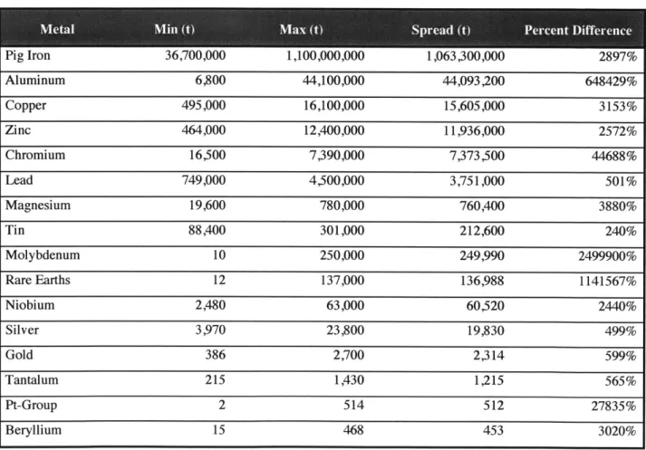
Table I Summary of statistical information related to production from 1900-2011'

Pig Iron 36,700,000 1,100,000,000 1,063,300,000 2897% Aluminum 6,800 44,100,000 44,093,200 648429% Copper 495,000 16,100,000 15,605,000 3153% Zinc 464,000 12,400,000 11,936,000 2572% Chromium 16,500 7,390,000 7,373,500 44688% Lead 749,000 4,500,000 3,751,000 501% Magnesium 19,600 780,000 760,400 3880% Tin 88,400 301,000 212,600 240% Molybdenum 10 250,000 249,990 2499900% Rare Earths 12 137,000 136,988 1141567% Niobium 2,480 63,000 60,520 2440% Silver 3,970 23,800 19,830 499% Gold 386 2,700 2,314 599% Tantalum 215 1,430 1,215 565% Pt-Group 2 514 512 27835% Beryllium 15 468 453 3020%

1 Not all metals had a starting value in 1900. See appendix (Table 20) for details on

(20)

a. Trends

The sixteen observed metals had very different levels of production. The least produced metal (beryllium) only had maximum tonnage of 468 metric tons from 1900 to 2011 whereas pig iron had maximum tonnage of 1.1 billion metric tons.

Aside from tin and molybdenum, the spread between the minimum and maximum production follows the same descending trend as the maximum. There are several factors that can attribute to the order of the metals in Table 1. Ease of extraction, end-user demand, and worldwide reserves are just a few.

Percent difference was calculated to determine which metals had increased the most in the last 110 years. Molybdenum, rare earths, and aluminum had the most significant differences between their minimum and maximum extremes. Conversely, tin, lead, and silver had the smallest percent difference between their minimum and maximum production.

(21)

Table 2 CAGR between minimum and maximum production Beryllium 1937 1956 20% RareEarths 1925 2006 12% Tantalum 1986 2004 11% Molybdenum 1900 2011 10% Aluminum 1900 2011 8% Niobium 1964 2008 8% PtGroup 1921 2006 7% Chromium 1900 2008 6% Magnesium 1937 2011 5% PigIron 1921 2011 4% Zinc 1921 2011 4% Copper 1900 2011 3% Silver 1946 2011 3% Tin 1945 2007 2% Gold 1900 2011 2% Lead 1900 2011 2%

To better understand growth, CAGRs were used. This introduced a temporal component allowing one to identify some of the fastest growing periods for the surveyed metals. Having either a large percent difference or a small difference between the years that the minimum and maximum production occurs can lead to a high CAGR. As such, the three metals with the greatest percent differences were also ranked in the top four highest spread CAGR metals.

Silver showed 65 years between its minimum and maximum, tin had 62, and lead had 111. Because these metals also had fairly small percent differences, their spread CAGRs all fell in the bottom 4 (3%, 2%, and 2% respectively). These metals had some of the smallest

(22)

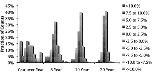
CAGRs between minimum and maximum points because they occurred at such different time periods. 45% - a >10.0% 40% - m 7.5 to 10.0% 35% 5.0 to 7.5% o330%₃₀ _{22.5 to 5.0%} L 25% o5 0.0 to 2.5% 020% 12% -2.5 to 0.0% u15% 10% -5.0 to -2.5% 5%-7.5 to -5.0% 0% - -10.0 to -7.5%

Year over Year 5 Year 10 Year 20 Year i <-10.0%

Figure 1 Histogram of Production CAGRs for Entire Metals Survey

From 1979-2011, production CAGRs were counted and presented in histogram format for all sixteen metals. The data approached a near-normal distribution with the mean just over 0.0%. Year-over-year, there were a number of instances where growth was over

10.0%. For five-year time-spans, the highest growth category fell from 17% of counts above 10.0% growth to only 5%. Observation of 20-year trending CAGRs makes it apparent that

collectively the metals production has grown moderately over this observed time period.

89% of all 20-year CAGRs were positive -78% of which were between 0.0 and 5.0%.

b. Volatility

To an extent, having an understanding of peak values and the range between them provides a context for volatility. Particularly if a spike happened in recent years, firms may choose to be more cautious with its use and even seek alternatives. Two types of analyses were carried out to quantify volatility.

(23)

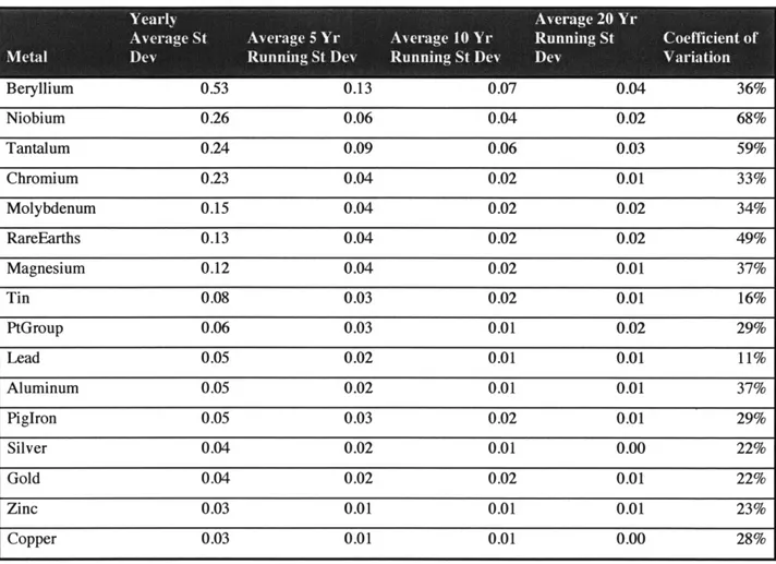
Table 3 Volatility Measures of Growth Rates for Production from 1979-2011

Beryllium 0.53 0.13 0.07 0.04 36% Niobium 0.26 0.06 0.04 0.02 68% Tantalum 0.24 0.09 0.06 0.03 59% Chromium 0.23 0.04 0.02 0.01 33% Molybdenum 0.15 0.04 0.02 0.02 34% RareEarths 0.13 0.04 0.02 0.02 49% Magnesium 0.12 0.04 0.02 0.01 37% Tin 0.08 0.03 0.02 0.01 16% PtGroup 0.06 0.03 0.01 0.02 29% Lead 0.05 0.02 0.01 0.01 11% Aluminum 0.05 0.02 0.01 0.01 37% PigIron 0.05 0.03 0.02 0.01 29% Silver 0.04 0.02 0.01 0.00 22% Gold 0.04 0.02 0.02 0.01 22% Zinc 0.03 0.01 0.01 0.01 23% Copper 0.03 0.01 0.01 0.00 28%

Using this measure for yearly growth, it appears that beryllium, chromium, niobium, and tantalum are the most volatile metals. Most of the other metals have standard deviations that fall below 0.10.

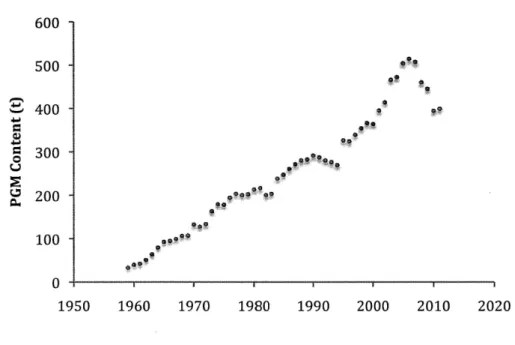
As would be expected, running averages of the CAGRs have declining variation with longer time periods. The only exception to this is platinum group metals. While its 10-year trailing CAGR was 1%, the 20-year trailing CAGR was 2%. This could be the result of the 20-year lagging CAGR taking points earlier than 1979 into consideration. From 1959 (the

(24)

first initial point in the CAGR calculations) to 1979, there is steady and high growth of production (an average of 10.3% year over year growth). The introduction and adoption of the catalytic converter, which uses platinum group metals, to the automobile occurred in the US between 1974 and 1975 (Gerard and Lave 2005). Over the entire 1959-2011 time frame, however, the average yearly growth rate is only 5.5% as a result of a strong decline of production beginning around 2007.

'0 0"' 9,' 0~O '*0 9', 9 a"t 1960 1970 1980 1990 2000 2010

Figure 2 Time-Series Production of Platinum Group Metals

The coefficient of variation does not follow the same descending trend as the standard deviation. Niobium, tantalum, and rare earths all had very high coefficients of variation while lead and tin had very low levels.

4-a 'a 4-h 0 600 -500 400 300 200 100 0 1950 2020

(25)

ii. Value

Table 4 Summary of statistical information related to value from 1900-20092

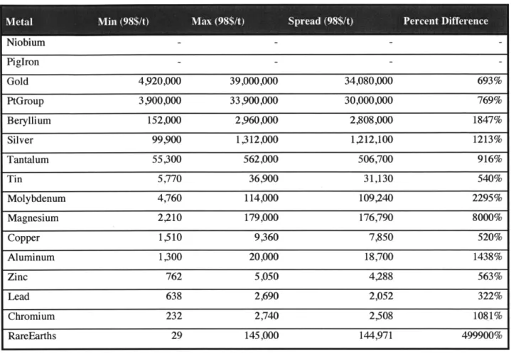
Niobium --PigIron - - - -Gold 4,920,000 39,000,000 34,080,000 693% PtGroup 3,900,000 33,900,000 30,000,000 769% Beryllium 152,000 2,960,000 2,808,000 1847% Silver 99,900 1,312,000 1,212,100 1213% Tantalum 55,300 562,000 506,700 916% Tin 5,770 36,900 31,130 540% Molybdenum 4,760 114,000 109,240 2295% Magnesium 2,210 179,000 176,790 8000% Copper 1,510 9,360 7,850 520% Aluminum 1,300 20,000 18,700 1438% Zinc 762 5,050 4,288 563% Lead 638 2,690 2,052 322% Chromium 232 2,740 2,508 1081% RareEarths 29 145,000 144,971 499900% a. Trends

Unfortunately, some of the metals had incomplete data sets for their values. After omitting niobium and pig iron from the survey, rare earths have by far the greatest percent difference between its minimum and maximum price. In 1933, a metric ton of rare earth oxide would cost $145,000, however, in 1939, the price plummeted to $29. Other metals with high percent differences included magnesium (8000% price drop) and molybdenum (2295% price increase).

2 Niobium and Pig Iron had a significant number of missing values so they were

(26)

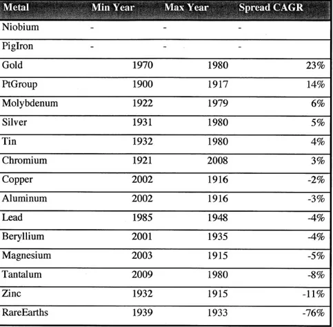
Table 5 CAGR between minimum and maximum values

Though values, on average, do not have as great of a percent difference between their minimum and maximum values as production, the CAGR of spreads tend to vary much more. Platinum-group metals (14%), gold (23%), rare earths (-76%), and zinc (-11%) all had the greatest smoothed growth trends and copper (-2%), chromium (3%), and aluminum (-3%) had the smallest.

In this case, the years at which minimum and maximum values occurred plays an important role. For production, the average minimum/maximum spread of years was 81. Also, the year of the maximum always happened later than the year the minimum occurred and most maximums for production occurred in the 2 1't century.

Niobium - - Pig~ron--Gold 1970 1980 23% PtGroup 1900 1917 14% Molybdenum 1922 1979 6% Silver 1931 1980 5% Tin 1932 1980 4% Chromium 1921 2008 3% Copper 2002 1916 -2% Aluminum 2002 1916 -3% Lead 1985 1948 -4% Beryllium 2001 1935 -4% Magnesium 2003 1915 -5% Tantalum 2009 1980 -8% Zinc 1932 1915 -11% RareEarths 1939 1933 -76%

(27)

For unit value, however, the average spread of years was 49 and approximately half of the CAGR spreads are negative as a result of the maximum value occurring before the minimum yielding price drops.

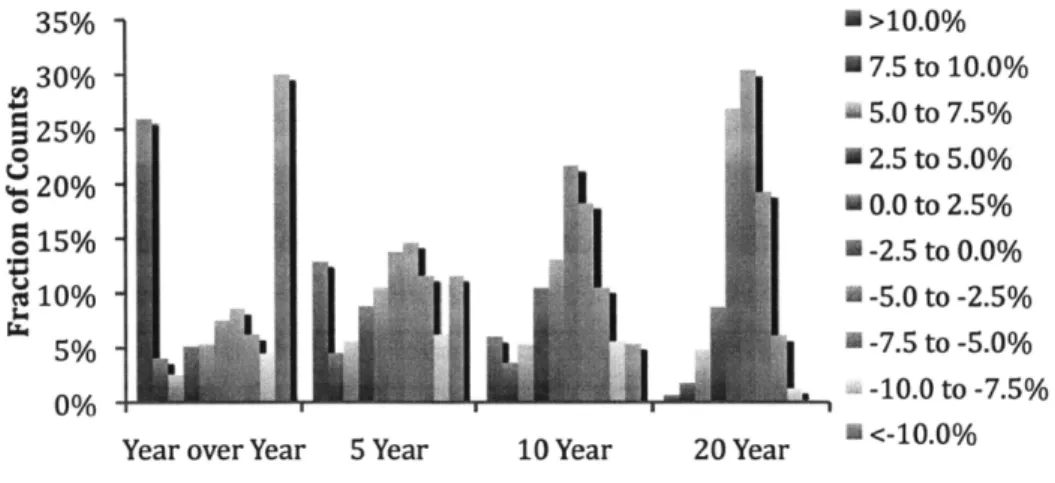
35% - N >10.0% 3 7.5 to 10.0% ~25% - 5.0 to 7.5% o 2.5 to 5.0% 20% 0.0 to 2.5% 015% - _{8 -2.5 to 0.0%} t10% U -5.0 to -2.5% 5% U -7.5 to -5.0% 0% A -10.0 to -7.5%

Year over Year 5 Year 10 Year 20 Year U<-10.0%

Figure 3 Histogram of Value CAGRs for the Entire Metals Survey

Though production growth appeared to be generally positive, value growths tended to be more negative. Yearly, growth rates were much more negative. 30% of values of rates from 1979-2009 were less than -10.0%. Also, compared to the production histogram, yearly value rates tended to fall more at the extremes. There were almost twice as many counts ±10.0% (56% versus 25%). Between five and ten year CAGRs, there was a shift from -2.5 to

-5.0% growth occurring most frequently to -2.5 to 0.0%.

(28)

Table 6 Volatility Measures of Growth Rates for Real Value from 1979-2009

Niobium--- PigIron----Tantalum 1.02 0.16 0.09 0.03 102% Molybdenum 0.57 0.23 0.11 0.06 112% RareEarths 0.52 0.11 0.08 0.03 40% Zinc 0.30 0.10 0.04 0.02 33% Silver 0.29 0.11 0.08 0.05 80% Chromium 0.27 0.07 0.05 0.03 34% PtGroup 0.24 0.08 0.04 0.02 27% Copper 0.24 0.11 0.05 0.02 39% Lead 0.23 0.09 0.04 0.02 39% Aluminum 0.21 0.07 0.03 0.01 31% Gold 0.21 0.09 0.07 0.05 40% Tin 0.21 0.07 0.06 0.04 61% Beryllium 0.21 0.09 0.07 0.03 43% Magnesium 0.17 0.05 0.03 0.02 26%

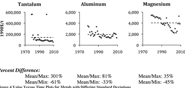
Among the 16 metals, tantalum's standard deviation of value growth was significantly higher (1.02 versus the 0.28 average of the others). Second to tantalum is molybdenum (0.57) and rare earths (0.52). The time-range has a great impact on the ranking of these metals. Only the most recent 30 years were considered. Tantalum is the only metal that has both its minimum and maximum unit values within this time frame. Though magnesium had one of the greatest percent differences between its minimum and maximum values, when constricted to the latest thirty years, its standard deviation of yearly growth is actually the smallest at 17%.

(29)

Tantalum 600,000 -S400,000 -% 200,000 - .. 0 1970 1990 2010 Aluminum 6,000 4,000 2,000 1970 % 1990 2010 6,000-4,000 2,000 0-19 Magnesium -,re. _e

7

'70 1990 2010 Percent Difference: Mean/Max: 301% Mean/Max: 81% Mean/Min: -61% Mean/Min: -33%

Figure 4 Value Versus Time Plots for Metals with Differing Standard Deviations

Mean/Max: 35% Mean/Min: -45%

Above are value versus time plots for three metals with standard deviations that were ranked first, middle-rung, and last. The percent difference between the mean (also denoted with dashed lines) and maximum as well as between mean and minimum were calculated. Magnesium had the lowest standard deviation and also has a much smaller percent difference (between mean and maximum) than either tantalum or aluminum.

IV. Analysis of Metals

In addition to interpreting results by relating a single metal to the full set, there are several ways to break up this survey of sixteen to make assumptions about broader trends. Those considered included whether a metal was on an open exchange or not, the rate of production, if the metal was base or precious, and the relationship between co-mined materials.

(30)

A. Metals Exchange

There are hundreds of commodities exchanges that exist worldwide. The four largest and most recognized for metals are LME, NYMEX, COMEX, and SHFE.

The London Metals Exchange (LME) is the largest market for options and future contracts on particular metals. The contracts can be temporally manipulated in a number of ways (from daily to multi-year expiry dates). Futures and options contracts are available for

aluminum, copper, tin, nickel, zinc, lead, aluminum alloy, steel billet, cobalt, and

molybdenum3.

Though the official commencement of this exchange was in 1877, the concept of metals exchanges was formalized in London in 1571 under Queen Elizabeth I's reign (Hart 2007). Forums were organized to bring together classes of people from financiers to

producers. During the Industrial Revolution, the market became globalized, causing a great deal of uncertainty regarding how much one would be able to sell ore brought from distant countries for. When the telegraph entered commercial use, it became possible for miners to notify those involved in the market of their cargo. After futures contracts became more controlled, buyers no longer had to worry about surprising increases in prices and sellers did not have to worry about drops in price (Hart 2007).

As London was growing and establishing its official exchange, merchants met in Manhattan to discuss the exchange of butter and cheese. With time, the variety of commodities grew and eventually the New York Mercantile Exchange, or NYMEX, was

(31)

established. Chicago became the other American hub for commodity exchanges and in 1933 COMEX (Commodity Exchange, Inc - a division of NYMEX) was formed (Goodman 2011).

A century later and halfway around the world, the Shanghai Metals Exchange (SHME) was established in 1992 and had markets for the non-ferrous metals copper,

aluminum, lead, zinc, tin, and nickel. The sheer size of China attributed to the growth of its

commodities exchanges. Particularly with the countries recent technological advance, China has become one of the world's largest producers as well as consumers of particular products. In 1999, SHME along with two other commodities exchanges combined to form SHFE (Shanghai Futures Exchange) in which copper, aluminum, zinc, lead, natural rubber, fuel oil, steel wire rod, steel rebar, and gold are currently traded. SHFE alone has become the third largest non-ferrous metals exchange in the world.

For the following analysis the sixteen surveyed metals were broken up into their respective categories. All analysis was done for the years 2009 (for values) or 1979-2011 (for production). It is worth noting that not all metals have been on open exchanges during that entire time period.

Table 7 Metals Exchange Categories

Aluminum, Copper, Aluminum, Aluminum, Beryllium, Chromium,

Lead, Molybdenum, Copper, Gold, Copper, Gold, Magnesium, Niobium, Pig

Tin, Zinc Silver Lead, Zinc Iron, Rare Earths, Tantalum,

Platinum-group metals'4

4_{Pt-group metals appear in NYMEX, however, they are the only metal from the}

survey in that exchange. As a result, these metals were classified as not being in an exchange.

(32)

Metals on an open exchange tend to be pricier than those that are not. This is likely because these metals are widely considered critical. From 1979-2009, all metals on an exchange had an average price of approximately $3.3M while those not on an exchange were over 1000 times cheaper (Table 8).

Table 8 Metals Exchange Value Statistics Averaged from 1979-2009

Clifcto Mi(8/t a $t)Aerg (98/t 209aue(8$t

Metals Exchange 1,765,981 6,875,280. 3,318,023 3,665,282 COMEX 2,045,453 10,080,298 4,123,786 6,041,093 LME 2,472 27,587 7,001 6,423 SHFE 2,013,396 9,753,005 4,047,087 5,951,670 No Metals Exchange 31,799 219,782 106,859 46,734

There were two surprising results from this study. Firstly, the price volatility of all of the metals categories are not widely different (Table 9) and secondly, the standard deviation of production growth has a strong bias towards metals not on open exchanges.

Table 9 Volatility of Value Growth from 1979-2011

Metals Exchange 28% 11% 6% 3% COMEX 24% 9% 6% 3% LME 29% 11% 6% 3% SHFE 24% 9% 5% 3% No Metals 31% 7% 5% 2% Exchange

(33)

Table 10 Metals Exchange Production: Volatility of Growth from 1979-2011

Yr Running, St 10 Yr Running St 20 Yr Running coefficient of

Classification Yearly St Dev Dev Dev St Dev Variation

Metals Exchange 6% 2% 1% 1% 0.25 COMEX 4% 2% 1% 1% 0.27 LME 7% 2% 1% 1% 0.25 SHFE 4% 2% 1% 1% 0.28 No Metals Exchange 22% 6% 4% 2% 0.44

Regarding production, metals on an open exchange appear to be significantly more stable than those not on a metals exchange. The standard deviation of yearly growth for non-market metals is many times greater than those on exchanges. Also, the coefficient of

variation is nearly twice as great. This is possibly due to the nature of futures contracts: they are put in place so that sharp changes in availability do not occur and therefore significantly impact the market.

(34)

23001

22001

21001

I:

1 9103M 20 1042012 I Date Cash buyer 7_400-... 2300-2100 1 9103 2 18esUr12 2 Date 2300 - -22 0 0 - ... 2100-2000... 1 9)=021 2 4 WNW1201 Date 3-months buyer 2400.--2300-' 2-200 19413Q0U12 1 WNW452 Date

15-months buyer 27-months buyer

Figure 5 LME Aluminum Futures Contract Rates for Varying Time Periods'

Above is a sample of futures contract price charts for aluminum. As with most purchases, it is advantageous to pay up front and be a cash purchaser. Even still, day-to-day prices can differ substantially. Though the trends for these four time periods are all similar, the scale of the y-axis changes quite a lot. A cash buyer would have paid approximately $2030 on 4/18/2012, $2090 for 3 months, $2190 for 15 months, and $2300 for 27 months ahead.

(35)

B. Production Rate

Economic theory would suggest that materials with high levels of production would also have fairly low values and vise versa. The sixteen metals were classified into three groups dependent on their levels of production as follows:

Table 11 Levels of Production

Loes Prdcto Meiu PrdcinGetetPouto

Beryllium, Gold, Niobium, Pt-group Metals, Silver,

Tantalum

Chromium, Lead,

Magnesium, Molybdenum, Rare Earths, Tin

Aluminum, Copper, Pig Iron

After segmentation and these metals differ by orders of

observation of their production statistics, it is apparent that magnitude.

Table 12 Production Statistics from 1979-2011 for Differing Production Levels

Greatest Production 159,200,000 386,733,333 219,418,788 386,733,333

Medium Production 936,233 2,226,333 1,411,010 2,200,500

Low Production 3,500 15,305 7,811 15,155

In 2011, the average of production for the highest category was over 25,000 times greater than those in the lowest production category.

(36)

Table 13 Production Volatility Statistics from 1979-2011

Yeary St 5 YrRunnng S 10 r Runing 20 Y Runing COefficient o

Clasifiatin Dv Dv S De StDevVariation.2 Greatest Production 4% 2% 1% 1% 0.31 Medium Production 13% 4% 2% 1% 0.30 Low Production 20% 6% 4% 2% 0.39

While the production is quite different from metal to metal, so is the degree of dispersion. Metals with low levels of production tend to be much more volatile. In terms of

standard deviation, the amount of possible change from year to year could be as high as 20%. Furthermore, the coefficient of variation is the highest.

Volatility results for production were sensible. Difficulty of extraction or low levels of natural reserves make the predictability of production hard to determine year-over-year. With this in mind, it presents the question of how difficulty of extraction is reflected in pricing.

Table 14 Production Value Statistics from 1979-2009

Greatest Production 1,037 3,222 1,769 2,685

Medium Production 2,870 28,900 7,938 7,617

Low Production 2,682,553 10,538,350 5,092,636 6,652,460

The average value of low-production metals is significantly higher than those with high levels of production. Referring to the table of metals values from 1900-2009 (Table 4),

(37)

gold, platinum-group metals, beryllium, silver, and tantalum are at the top of the list6_.

Medium and high production level metals were in mixed positions following the top five. Perhaps after a particular threshold of production level, other factors become weighted more heavily in the valuation of a material.

Table 15 Value Volatility Statistics from 1979-2009

Greatest

Production 23% 9% 4% 2%

Medium

Production 33% 10% 6% 3%

Low Production 39% 11% 7% 4%

While the value of a metal may be high, regardless of its production level the

variation is fairly similar. Low production metals have a yearly growth standard deviation of 39% compared with their high growth, high production counterparts that have a dispersion of 23%. Expectedly, if a metals level of production has consistent growth, prices are much easier to set and will tend to vary less. For the coefficient of variation, low production metals had an average 0.58 but with a wide spread. Platinum-group metals had a coefficient of variation of only 0.27 while tantalum's was 1.02. The other two categories did not have as much difference between all of the metals in their categories.

6 Niobium had some missing value data and was, therefore, excluded from the survey

I

0.35

0.52 0.58

(38)

C. Base and Precious Metals

Base metals tend to be abundant in nature and therefore in high use across various industries. Unfortunately, they also tend to corrode and oxidize easily particularly in a moist environment. According to the US Customs and Border Protection Agency, of the surveyed metals, eleven are classified as base metals (Table 16). Conversely, precious metals are found in low concentrations in Earth's crust and naturally occur in a non-oxidized state.

Table 16 Base and Precious Metals

Aluminum, Beryllium, Chromium, Copper, Lead, Gold, Pt-group Metals, Silver Magnesium, Molybdenum, Niobium, Pig Iron, Rare

Earths, Tantalum, Tin, Zinc

Table 17 Production Statistics for Base and Precious Metals (1979-2011)

Base 40,762,474 98,823,818 56,235,216 98,811,419

Precious 4,037 9,005 6,317 8,966

The production of base metals is approximately four orders of magnitude greater than that of precious metals.

Table 18 Production Volatility for Base and Precious Metals (1979-2011)

Base 15% 4% 3% 2% 0.34

(39)

Gold and silver's wide use for currency exchanges adds another factor for its demand. Because of both their difficulty in extraction and use for monetary systems, precious metals tend to be much more expensive than their base metal counterparts. In 2009, precious metals on average cost about $10.9M per metric ton (1998 dollars) while base metals cost $35,723 per metric ton.

Table 19 Price Statistics for Base and Precious Metals from 1979-2009

Base 19,530 141,025 65,263 35,723

Precious 5,293,000 20,570,667 9,940,069 10,983,000

D. Case Studies

In the following sections, tantalum and niobium were researched further because of their distinct historical production and value trends. Additionally, these two metals are co-mined (with tin in some ore bodies). To compare their statistics to an industrial metal, a more detailed account of copper's statistics can be found in the appendix (Figure 18-Figure 21).

i. Tantalum

Tantalum showed multiple instances of extreme year-over-year change in the past 30 years that inspired a closer look at its activity.

There are three different forms in which tantalum can be bought: tantalum

ore/concentrate, tantalum oxide/salts, and capacitor-grade tantalum powder. Capacitor-grade powders typically make up about 25% of end-use. The material's high melting point and

(40)

resistance to corrosion make it an ideal material for use in extreme environments. Electronic applications tend to dominate use. Over time this metal has also been used as a substitute for platinum.

The defense industry also makes heavy use of tantalum and (at least in America) it is classified as a critical and strategic metal. Aluminum, titanium, tungsten, and zirconium can all be used as a substitute in the defense industry but each of these options has different penalties: either they are more expensive than tantalum or the performance is not as great.

Value

Though tantalum is not traded openly on any metals exchanges, Ryan's Notes supplies value data to USGS by surveying market makers. Consumers, traders, and

producers are all questioned before a price point is established. The level of specification and use case are some of the largest factors affecting the price of tantalum.

From the mid-twentieth century, tantalum's value has grown and fallen leading to an extreme spread in a short period of time. In the 1960s, tantalum's use in applications specific to the defense industry was first discovered. Increased demand caused inventory stockpiling through the early 70s and affected pricing as a result. Stockpiling continued through the decade, but in 1979 and 1980, demand outpaced the amount produced thereby skyrocketing prices to the highest point seen in this metals history. These high costs were then passed on to end users further down the supply chain so consumers discovered opportunities for substitution and use declined. In many electronics, tantalum was replaced with aluminum.

By 1986 these prices were quite low as a result of demand-reduction and the stockpiling that occurred in the early 1980s. Stockpiling also explains the rise and fall of

(41)

prices without a corresponding rise and fall of production. Also, though the electronics sector was growing during this time (cell phones, video cameras), miniaturization of these products meant less tantalum used per unit so there was not a corresponding growth of its demand. 600,000 -500,000 -' 400,000 300,000 m 200,000 100,000 . . .*... 0 1955 1965 1975 1985 1995 2005 2015

Figure 6 Bivariate Fit of Tantalum Value by Year

Production

Mines in South America and Australia have dominated the production of tantalum. Referencing the different factors that can influence scarcity (Alonso, Gregory et al. 2007), three very different situations changed the rate of tantalum's production.

In 2008 and 2009, some of the largest tantalum mines in Australia, Canada, and Africa were closed for economic reasons. As a result, in 2009, the Democratic Republic of Congo and Rwanda were responsible for 50% of the global tantalum production.

(42)

significant price jumps. In the United States in accordance with the Conflict Minerals Law, electronics companies are required to disclose the sources of their raw materials. In recent history, more countries have advertised tantalum as a critical material encouraging the development of institutional changes that might moderate tantalum trading, pricing, and production levels.

Several countries have openly admitted their desire to find alternatives to tantalum. China - a country that purchased 80% of Brazil's tantalum supply in 2008 - has also put a significant amount of money and effort into the discovery and establishment of new mines in Africa (Tanquintic-Misa 2012). 1600 -1400 . 1200 . 1000 0 800 . -400 . .. * *. * ee e . * -e. * 200 * 0 1955 1965 1975 198 1995 2005 2015

Figure 7 Bivariate fit of tantalum production by year

1979, 1980, and 2000 are all years with outlying prices. From research of Tantalum's temporal trends, stockpiling and end-use demand were the main factors that resulted in these effects. Though there does not appear to be any strong direct correlation between values and production, after comparing the year over year growth in value and production, there are

(43)

some more noticeable behaviors. Upon fitting a line of best fit, the slope is greater than one suggesting that a marginal deviation in the rate of production has a large effect on the yearly growth of the value.

600% 500% 400% 300% -0 200% -Ca 100% -. -60% -40% *-20% 100% 0O 20% 40% 60% 80%

Production Year Over Year Growth

Figure 8 Price growth versus production growth for tantalum

There is, however, a high likelihood that there is a time lag between these supply and demand factors. It is difficult to determine if availability causes changes in price (standard economic view) or if some end-use demand further down the supply chain most heavily impacts the relationship in Figure 8.

(44)

80%

- Yearly Prodn Growth

60% -- 5 CAGR Prodn 10 CAGR Prodn 40% -- 20 CAGR Prodn 20% 0 % -20% -40% -60% 1975 1980 1985 1990 1995 2000 2005 2010

Figure 9 Trending production CAGR for 1, 5, 10, and 20 years for tantalum

In the last thirty years, production growth has fluctuated quite a lot. Tantalum's standard deviation of growth was in fact the third highest in the metals survey. When longer periods of time are considered, the volatility is lessened and it becomes easier to make assumptions about trends. In observation of the 20-year trending CAGR, world wide production growth has been increasing over time. There are very few instances of negative growth. Since the beginning of the 2 1't century, the growth rate seems to have plateaued at

(45)

1,600 Other Transportation 36% t

Machinery Electronic components

p1,400 ---- Worldwide Production 21,200 a1,000 - 242% a ~178% - w . 60 200 200 LO r N % q M- f L(n t N V-4 rvn Ln t N r_1 M- v rN Nl N" oo oo 0 0 C % ON 0 ON 0D 0D ON C% ON ON ON ON ON 0% ON 0% ON ON ON 0 0D -4 r-4 r-1 r-1 r-4 -4 -4 -4 -4 r-4 -4 -4 -4 N1 C1 Year

Figure 10 U.S. Tantalum End-Use Statistics and World Production Data

Above, the U.S. use of tantalum is charted and broken up into four industrial

categories: electronic components, transportation, machinery, and other. End-use is difficult to approximate and the USGS derives these statistics by applying estimated end-use

percentages based on Mineral Commodity Summary publications (U.S.G.S. 2011).

Until 1989, U.S. end-use almost always outpaced world production. While U.S. use levels are high, the country has not had a significant amount of production since 1959 because the ore grade was very low (Cunningham). The yellow boxes highlight the ratio between U.S. end-use and world production. In 1984, use was nearly 2.5 times greater than the amount produced that same year (or any year from 1975 to 1984). As discussed earlier, high demand and high prices lead firms to seek substitution opportunities and the following year use was only 15% greater than the amount produced. In the 1990s, production took off without a matching increase in demand or use.

(46)

Though there was anticipated growth of the electronics sector, the data was not representative of that. During the entire surveyed period of time, electronics had an average percentage of total use of approximately 66%±3%, machinery had an average percentage of 21%±2%, transportation's average was 8% 1%, and the other category had an average of

5%±2%. Though the time period from 1975 to 2003 had entry of many new technologies,

the use mix remained fairly constant.

ii. Niobium

Niobium derives its name from the Greek mythological figure Niobe - the daughter of Tantalus. For quite some time, scientists thought that niobium and tantalum were actually the same metal. This was primarily assumed because of the difficulty of isolating the two similar metals. Though the mineral was initially discovered in 1734, it would not be until

1864 that Wilhelm Blomstrand would be able to isolate niobium and it became identified as its own element (Britannica 2012).

Value

The significance of this metal is its resistance to corrosion and heat conductivity. While tantalum price was heavily driven by end-use demand, niobium's price is affected by the amount of columbium mineral available. According to USGS specialists, when

(47)

60,000 50,000 40,000 30,000 20,000 10,000 0 -1955 .. ** *. 0 . 0 ** **..*.... 1965 1975 1985 1995 2005 2015

Figure 11 Bivariate fit of niobium price by year

Contrary to that claim, in comparing yearly growth of price with yearly production growth, the data appears to be scattered and random. It is likely that it

takes some time before price effects are realized from production level changes.

80% 60% 40% 20% -20% -40% -4% -2% 0 4

.

a 0 S S S* 0 0% 2% 4% 6% 8%

Production Year Over Year Growth

10% 12%

Figure 12 Price growth versus production growth for niobium

U) Cu 0 'I so 6-Mu 6. 0 _a

(48)

Production

Niobium also has several applications in the defense industry. It is therefore classed as a strategic metal and in the late 1950s the United States initiated a program to increase worldwide discovery and production of tantalum and niobium ore. The result of this was the discovery that the majority of domestic deposits are of low grade and this ultimately led to the termination of this program. As a result, prices fell and columbium (one of niobium's feed minerals) exploration decreased as well.

Unfortunately, recycling is not a significant source of niobium so consumers are very reliant on primary production. The discovery of the steel strengthening effects of small

amounts of columbium in the 1960s had a direct impact on both the value and production of the metal. Pyrochlore deposits were established in Brazil and Canada around this time to sustain the growing demand for columbium.

70,000 -.**** 60,000 -'z 50,000 -40,000 * 30,000 * 20,000 * 10,000 . ,.** 0 1955 1965 1975 1985 1995 2005 2015