Distribution of air mass thunderstorms in New England.

TC>

DISTRIBUTION OF AIR MASS THUNDERSTORMS IN NEW ENGLAND

John James Owens, Jr.

A.B., Clark University (1950)

SUBMITTED IN PARTIAL FULFILLMENT OF THE REQUIREMENTS FOR THE DEGREE OF

MASTER OF SCIENCE

at the

MASSACHUSETTS INSTITUTE OF TECHNOLOGY June, 1966

Signature of Author

Department of Meteorology, June 19, 1966

Certified by ...

Thesis Supervisor

Accepted by ... c... .

Chairman, Departmental Comittee on Graduate Studer.ts A- 17 !:-) (-, g C 'N

MITLibraries

Document Services

DISCLAIMER OF QUALITY

Due to the condition of the original material, there are unavoidable

flaws in this reproduction. We have made every effort possible to

provide you with the best copy available. If you are dissatisfied with

this product and find it unusable, please contact Document Services as

soon as possible.

Thank you.

Pages are missing from the original document.

No page numbered 58 in this thesis.

--DISTRIBUTIONS OF AIR MASS THUNDERSTORMS

IN NEW ENGLAND

by

John James Owens, Jr.

Submitted to the Department of Meteorology on June 20, 1966 in partial fulfillment of the requirements for the Degree of Easter of Science.

ABSTRACT

The SCR-615-B radar data was used to locate air mass thunderstorms and hailstorms in New England. A total of 64 out of 71 air mass and 148 non-air mass thunderstorm days between March and October of the years 1958 through

1965 had suitable radar data. A majority, 108, of the non-air mass

thunder-storm days were accompanied with cold fronts or quasi stationary fronts.

Various synoptic parameters that indicated stability and moisture on the air mass days were recorded. It was fourd that 61 out of 64 days with air mass thunderstorms had sea breezes and 40 out of 64 days had confluence at 500 meters.

The -area covered by the radar was divided into a grid of ten-by-ten mile squares, and the frequency of occurrences, formation and dissipation of thunderstorms and hailstorms in each square were recorded. Detailed maps

are presented showing the distributions for days grouped according to the 500-mb flow. Areas of maximum frequency of occurrence were about a band

about 30 miles wide extending from just east of Concord, N.H. to central Massachusetts and northern Rhode Island, the eastern sides of major river valleys and near certain mountains. Regions of minimum frequency of occur-rence were east of the 500-ft MSL contour in Maine and the south coast of

New England and. its adjacent coastal waters from New HavenpConnecticut to

Cuttyhunk IslandaMassachusetts.

Maps are presented showing the tracks of thunderstorms, They were nearly all parallel to the 500-mb flow and most of the tracks had lengths

less than 15 miles. Tracks that were longer than 30 miles were made by relatively large cells with one dimension greater than five miles.

Thesis Supervisor: Dr. Pauline M. Austin Title: Research Associate

A C K N

0

W L E D G E M E N T S

The author

is

indebted to Or. Pauline

M.

Austin for her

guidance, suggestions ani comments in interpreting the M.I.T. radar data and

preparing

the thesis. I wish to

thank Professor Erik

L.

Mollo Christensen for

his comments on

Lee and

gravity waves.

Mr.

Spiros Geotis kindly

gave guidance

on the characteristics and operational

use of

the M.IoT,

radar, Mrr

Steven

A.

Ricci prepared the final copies

of

the numerous figures and diagrans.

The

author wishes to thank Mr.*

Edward E. Begin, Chief Engineer of the lew Bedford

Water Works

and Mr.

Charles O'Leary, working foreman

of

the Taunt(n Water

Works for their comments on the local hydrology and providing special

thunderstorm observations.

I

wish to

thank

Mr. Edward C. Nelson, of the Sync ptic

Meteorology Department for typing this manuscripto

TABLE OF CONTENTS

Page ABSTRACT ... a .. 0.0.00.0000.00.0.00000... 0. 01000000.

ACKNOWLEDGEMENTS ... iii

TABLE OF CONTENTS ... iv-v LIST OF FIGURES ... . . .. ... vi-viii LIST OF TABLES .... ... ... a ... ... ... ix

INTRODUCTION ... ... ... ... . . 1

PREVIOUS STUDIES OF THE DISTRIBUTION OF THUNDERSTORMS IN NEW ENGLAND ... ... ... . ... .. .. 5

A. General Topographical Features ... ... 5

B. Climatological Studies of Thunderstorms and Hailstorms 5 C. Short Period Investigations ... 14

EFFECT OF TERRAIN ON AIRFLOW ...0000000000*0000 17 A. Orographic and Thermal Effect ... 17

B. Lee Wave Effect . 17 DATA AND METHOD OF ANALYSIS . 21 A. Use of Radar to Locate Thunderstorms ... 21

B. Radar Data used in this Study ... ... 22

C. Selection of Air Mass Thunderstorms ... 24

Do Method of Analysis . 24 RESULTS o.o....oo.o ooooo...oooo o00o. ooo... . 26

A. Number of Days when Thunderstorm Echoes were observed. 26 B. Characteristics of Air Mass Thunderstorm Days ... 26

C. Characteristics of Air Mass Cells ... 28

D. Cell Motions ... 0 .0 ... 0 ... 31

E. Detailed Topography of Area ... .... ... 35

F. Geographical Distribution for all Air Mass Thunderstorms. 42 G. Distribution for Days with Southwest Flow ... 51

H. Distribution for Days with Northwest Flow . 65 I. Distribution for Days with Closed Lows or Deep Troughs at 500-mb ... . ... .000 .00000 69 J. Distributions for other Directions of Flow . 77 K. Discussion of Results ... 77

Page

CONCLUSIONS ... ,6....6.90---0...6... 84

APPENDICES 00. 00. 00. 0.. 09.000...0... 87 A. List of Days when the SCR-615-B recorded Cells with

log Ze> 4.5, which were not of the Air Mass Type . . . . 87

B. Number of Days in each Year, from March through November

when the SCR-615-D Radar recorded Cells with log Ze> 4.5. 91

C. List of Days and their Characteristics when the SCR-615-B

recorded Air Mass Cells with log Ze

>4.5

D. Characteristics of Radar Echoes from Air Mass

Thunder-storms ...--- ... 106

LIST OF FIGURES

Page

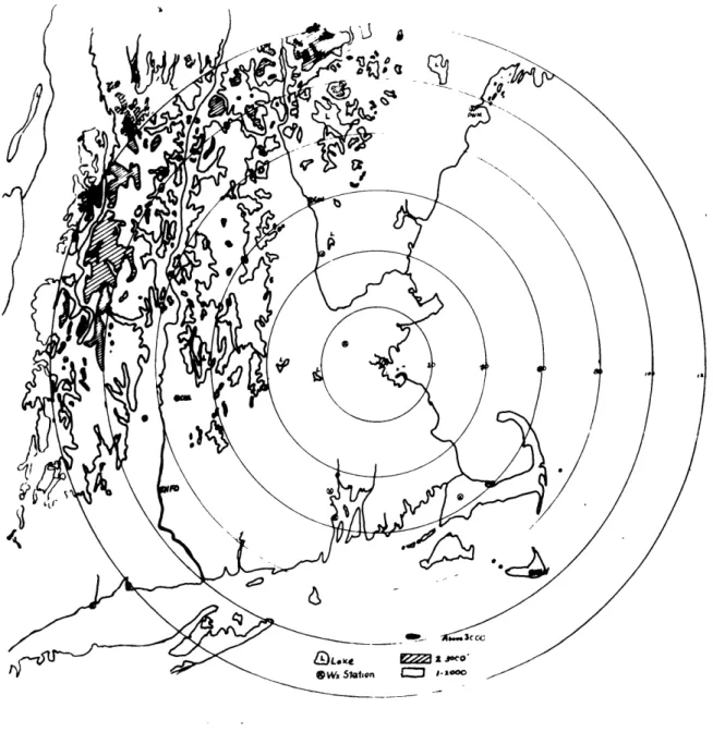
Fig. 1. Ganeral terrain map of New England. Range markers in

statute miles ... ,... 6

Fig. 2. Smoothed topographical map of New England. Elevations

in hundreds of feet. (From Tweedy, 1965) ... 7

Fig. 3. Average annual number of thunderstorm days based on more

than 20 years of record ... 9

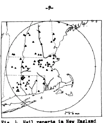
Fig. 4. Hail reports in New England based on the years 1953 through

1962 .. ... 0.0.00000000000.0.0.0.0.0.00900.00 9 Fig, 5. Areas with highest hail crop insurance rates. Legend:

X tobacco; Z general crops . 9

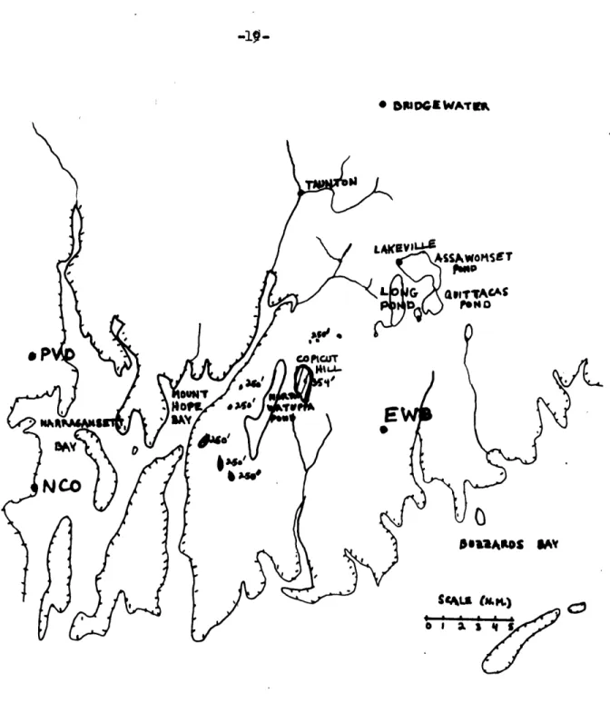
Fig. 6. Major terrain features near the watersheds of the ponds at

Lakeville, Massachusetts . 19

Fig. 7. Average orientations of air mass cells with log Ze 4.5 in

each lx10 mile square ... 30

Fig. 8. Distance between large cell groups (miles) . 30

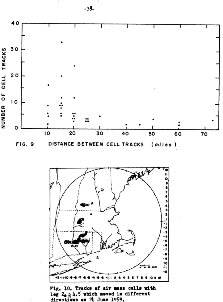
Fig. 9. Distance between cell tracks (miles) ... 33

Fig. 10. Tracks of air mass cells with log Ze> 4.5 which moved in

different directions on 24 July 1959 ... *...0.. 33

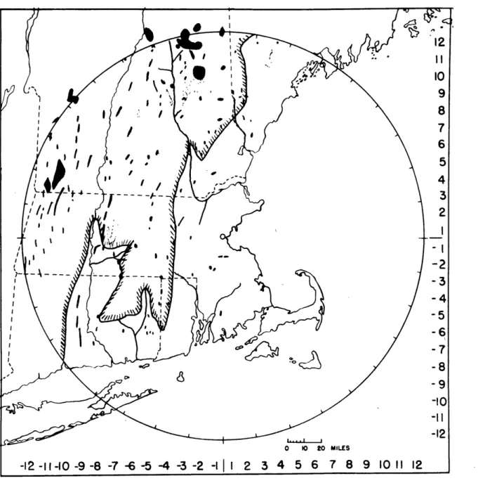
Fig. 11. Map showing topographical barrier, 500-ft contour, and major

rivers and lakes (dotted areas) ... 37

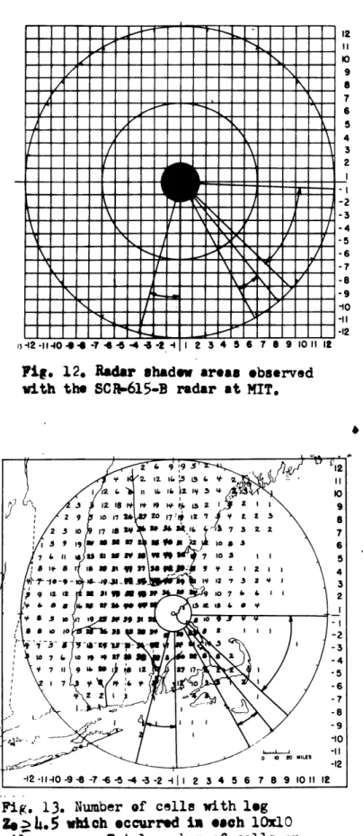
Fig. 12. Radar shadow areas observed with the SOR-615-B radar at

M.I.T. ... .. .. ,... 41

Fig. 13. Number of cells with log Ze A4,5 whioh occurred in each

l0xlO mile square. Total number of cells on 64 days was

3878 0 0 .. . a 0 0 0 0. 0. 0 00 0 .0. 0 0 0 0 0 . . . 0 0 0 .0 . 0 0 . 0 0 0 41

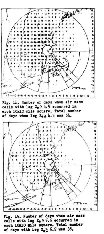
Fig. 14. Number of days when air mass cells with log Ze,4.5 occurred in each l0xlO mile square. Total number of days when log

Ze 4.5 was 64 ... 43

Fig. 15. Number of days when air mass cells with log Zet 5.5 occurred in each 10x10 mile square. Total number of days when log

Ze? 5.5 was 38 ... .... ... 43

Fig. 16. Number of cell formations when log Ze increases to 4.5 in

Page Fig. 17. Number of all dissipations when log Ze decreases to

below 4.5 in each 10x10 mile square ... 46

Fig. 18. Total time in tens of minutes when cells with log

Ze> 4,5 were in each l0xlO mile square ... 48 Fig, 19. Total time in tens of minutes when cells with log

Ze)X5.5 were in each 10x1O mile square ... 48

Fig. 20. Locations and intensities of cells with log Ze 6.0 0... 50

Fig. 21. Number of days when air mass cells with log Ze>.4.5

occurred. 500-mb flow: SW to W. Total number of days: 47. 50

Fig. 22. Number of days when air mass cells with log Ze?5.5

occur-red. 500-mb flow: SW to W. Total number of days: 29 .... 52

Fig. 23. Number of cell formations when log Ze increases to 4.5 and

500-mb flow is southwest to west ... 52 Fig. 24. Number of cell dissipations when log Ze decreases to below

4.5 and 500-mb flow is southwest to west ... 54

Fig. 25. Total time in tens of minutes when cells with log Ze? 4.5

were in each 10xlO mile square. 500-mb flow: SW to W .... 54

Fig, 26. Total time in tens of minutes when cells with log Ze2 5.5

were in each l0xl0 mile square. 500-mb flow: SW to W .... 56

Fig. 27. Cell tracks when log Ze04.5 and 500-mb flow is southwest.

Total number of days: 10 ... 56

Fig. 28. Cell tracks when log Ze 4.5 and 500-mb flow is southwest.

Total number of days: 6. Range: 60 miles ... 61

Fig. 29. Cell tracks when log Ze24.5 and 500-mb flow is west

south-west. Total number of days was six ... 0... 61

Fig. 30. Cell tracks when log Ze.4,5 and 500-mb flow is west.

Total number of days was 22 ... ... 62

Fig. 31. Cell tracks when log Ze 4.5 and 500-mb flow is west.

Total number of days: 8. Radar range: 60 miles ... 62

Fig. 32. Selected cell tracks when log Ze is slightly less than 4.5. 500-mb flow: SW to WSW. Total number of days: 4.

Radar range: 60 miles ... 63

Fig. 33. Number of days when air mass cells with log Ze?4.5

occur-red. 500-mb flow: NW. Total number of days: 11 ... 63

Page

Fig. 34. Number of days when air mass cells with log Ze 5.5

occurred. 500-mb flow: NW. Total number of days: 6 64 Fig., 35. Number of formations of air mass cells when log Ze

increased to 4.5 and 500-mb flow is northwest ... 64

Fig. 36. Number of dissipations of air mass cells when log Ze

decreased below 4.5 and 500-mb flow is northwest ... 66

Fig. 37. Total time in tens of minutes when air mass cells with

log Ze24.5 were in each lOxlO mile area. 500-mb flow: NW. 66

Fig. 38. Cell trac& when log Ze 4.5 and 500-mb flow is west

north-west. Total number of days: 6 ... 68

Fig. 39. Cell tracks when log Ze> 4.5 and 500-mb flow is northwest.

Total number of days: 5 ... 68

Fig. 40. Number of days when air mass cells with log Ze24.5 occurred with closed low or deep trough at 500-mb. Total number of

days: 8 ... ... 8 000. 00.00.. 0000000000 70

Fig. 41. Number of formations of air mass cells when log Ze increased

to 4.5,with closed low or deep trough at 500-mb ... ,. 70

Fig. 42. Number of dissipations of air mass cells when log Ze de-creased to below 4.5, with closed low or deep trough at

500-mb .. ... ... ... ... ... ... 71

Fig. 43. Total time in tens of minutes when air mass cells with log Ze 4.5 were in each square when there was a closed

lo or deep trough at 500-mb . 71

Fig. 44. Total time in tens of minutes when air mass cells with log Ze 5.5 were ii each square when there was a closed

low or deep trough at 500-mb ... . 74

Fig. 45. Axis orientations of air mass cells when log Ze>4.5, and

when there was a closed low or deep trough at 500-mb ... 74 Fig. 46. Tracks of cells with log Ze 4.5 for one day when 500-mb

flow was north .... . 0... 0 00 0 0 0.0.0 0 .0 0000 0 0.0 00 76 Fig. 47. Tracks of cells with log Ze 4.5 for two days when 500-mb

flow was south southwest ... ooooooooo 76

Fig. 48. Tracks of cells with log Ze 4.5 for one day when 500-mb

flow was south southeast ... 78

70 SUO-F4Az8Bqo jupwa pus 8ouls Jo uQ0Taud1UQo 06 a~qujL se404000000000 9VD8V GtT~ OTXOX ;o sanv38j o3dvagodoJ, 08 O1q131 90 .. 4nT13eUUO3 'ttftO49PPTW IJ38U SUOIDG0OTP ZuO8OZITP uT POAOUI S1100 I0~I 696T Stnr :P fO rvPuT OZTe igodda LA ONq01 D's 00000000000096000000000 p0.tafloo SITT8 B$suI

J.Vr

(qm-00g

04~

quz-099)

Szuetqs UOT~tOJP

PUM

iDq

spoods PUT&

qiu-00g

sAvr'

1. INTRODUCTION

Almost all reliable observers are aware of preferred areas for thunder-storms, but there has rarely been any quantitative and objective assessments

of the actual frequencies of occurrence within these areas.

The author decided to study only air mass thunderstorms as some previous studies have been of squall lines and thunderstorms associated with cold fronts in New England. Air mass thunderstorms usually have a smaller areal coverage than other types and are simpler to analyze. Moreover, theoretical considera-tions and European studies indicate that there would be more likelihood for preferred areas of occurrence, as well as for formation and dissipation because they would be less influenced by the larger scale circulation.

This type of study is best done by radar analysis, as a radar can

locate all thunderstorms and follow their life cycle. Data accumulated by the Weather Radar Research project at the Massachusetts Institute of

Tech-nology was used for this project.

There are many benefits to be derived from this type of research and it could be expanded into a climatological study. If there are preferred areas of thunderstorm activity, weather forecasts could be improved and be more specific regarding areas of possible occurrence. This would be important in the summer when the majority of inland New England precipitation is of the showery type. Climatological statistics could then be suitably modified and this information would be useful to agriculturists and insurance companies.

It might also assist water conservationists in planning distribution of water and building of dams to relieve water shortages and mitigate

-2-The question

of

whether or not thunderstorms will occur in some

general area depends on atmospheric conditions rather than topography.

The ideal conditions for occurrence of air mass thunderstorms are

instab-ility, con- :rgence at low levels, orographic uplif

.,

low level heating

and suffic :..nt moisture, while large hail requirer

in addition, strong

wind shears and a freezing level near or above the 'Aoud base.

There is little doubt that orography and elevations do have an

effect on precise locations of thunderstorms. A

number of studies

of this

effect have been made

in Europe

and the

mid

western united States.

The author noted, during the years 1953 through

1957

and 1961 through

1964, that in the densely

spaced (approximately

15

miles apart) network in

the United Kingdom, meteorological stations in positions with upslope flow

reported more thunderstorms and heavy showers than those with no upslope flow.

Ludlam (1962) studied the 18 June 1957 thunderstorms

in

England and found

that hill and sea breeze circulations

were pronounced over

peninsulas. There were definite preferred areas for thunderstorm occurrences

to the

lee of the highest hills

and

ridges of high ground.

In Germany, Trautmann (1960) studied the hailstorms in Bayern during

the period 1952 through 1956. The regions

most highly

affected include the

Ober Bayern of the Alps where the elevation is over 2000 feet, the hilly

Mittel Franken near Nurnberg where the elevation

is

over

2000 feet and the

upper course of the river Frank Saale near Schweinfurt.

Ortmeyer (1952) in a study of the 1924 through 1941 data found streaks

of hail damage parallel to the Era Mountains, showing the effect of topography.

-3-Schleusener (1961) found that hail genesis regions in northeastern Colorado during 1960 and 1961 were in the areas of topographical uplift, when the cloud bases originated below 5000 feet MSL.

Zinkiewicz (1955) studied 2,257 hail cases during the period 1946 through 1950 in Poland and found the greatest frequency of hail on the

high plains.

Frisby (1962 and 1963) found that 72% of the Upper Great Plain "straight line" hailstorms of 1951 through 1960 originated over higher ground. When all types _{of hailatorms were included however, the number of}

storms over equal areas of hill and valley were about identical. A study of 1961 hailstorms showed no clear indication that elevation played any part in hailstorm origins.

Stout and others (1959) stated that in the High Plains of the United States, there is a definite increase of hail crop damage losses with in-creasing elevation. However, they found that in Illinois, where there is not much difference of elevation, that there is a marked regional variation. Stout (1962) suggested that it could be explained by microphysical features,

such as surface slopes, terrain roughness and land use.

There is some evidence that land use affects the frequency of thunder-storms. Certainly the ground temperature would have some effect on convective activity and depends on the exposure to sunlight, the type of soil, moisture. and other factors.

Trautmann (1960) found that arable lands in Bayern were more severely damaged than forests and meadows.

Zinkiewicz (1955) stated that in the high elevations of Poland, the

forests may decrease the convective activity and reduce the hail frequency

In this study, detailed maps have been constructed showing the frequency of occurrence of air mass thunderstorms and hailstorms in New England, as indicated by quantitative radar observations. The number of storm formations and dissipations have also been mapped. The results were then compared with the various terrain features.

-5-2.

PREV1O1

STUDIES OF 7HE DISTRIBW101 01 THUNDERSTORMS IN NEW

GAN

A. Geeral topographical features.

Since terrain does have

an effect on thunderstorm activity*, a detailed

study was made of the terrain within a radius of 120 statute miles of M.Z.T.

Figure 1,

"General terrain map.

of New England", shows the predominan* White

Mountains of central New Hampshire, the Green Mountains of Vermont, the

Berkshire Hills of Western

MassachusettS and scattered

mountains in

south-western New Hampshire and central Mseachusetts east of the Connecticut River.

Figure 2, "Hlevations in hundreds of feet",, shows smoothed contours at more

frequent height intervals.

B. Climatological Studies of thunderstorms and hailstorms.

The typical thunderstorm and hail frequency charts are bsed on reports

from widely scattered weather stations that provide only point frequencies

and may not be representative, even locally.

The typical U.S. Weather Bureau first order station now

has a large

"background" noise so that distant thunder (thunderstorm reported as observed)

cannot be discerned as

readily

as desirable.

'Thunder is seldom heard farther

than 15 miles, with 25 miles the approximate upper limit and 10 miles being

a fairly typical range of audibility.

In addition to regular station reports, some severe weather incidents

are reported by private individuals.

Recently there has been an improved

reporting system as well as an interest by the general public in reporting

severe weather.

As more areas become heavily populated, more severe weather

reports can be expected.

The U.S. Weather Bureau makes cost estimates of

damage and

uses

a newspaper clipping service for their "Local Storm" data

Fig.

1.

General

terrain map

of

New England.

-.7j.

Elevation in hundreds of feet

Values indicated are averages of heights of 4 surrounding intersections of 15' of longitude and latitude.

Fig.

2. Smoethed tepegraphical map

of New

England, Elevations in hundreds of feet.

The Crop-hail Insurance Actuarial Association gathers reports of crop

damage by hail and bases hail crop insurance rates on these data. The data

indicate that one hailstorm may be more damaging than several others, depending on wind force, crop maturity, size and number of _{hailstones, nature of exposed} property and many other factors. Detailed, more reliable hail climatological studies have been made in the Mid West and Illinois, based mainly on crop

damage reports.

Another important consideration in determining the actual distribution

of hail is the ratio of "area" to "point" frequency of hail occurrence where

area frequency is based on an increased network density. Although present statistics are based on point frequencies, it appears that area frequency would be more accurate. Alfred Angot of the French Meteorological Service estimated

that an ideal reporting network for obtaining realistic area frequencies of hail

should be one station for each four square miles.

Several studies have been made of the hail to thunderstorm ratio and they

all indicate that the ratio decreases with increasing network density, Table 1, "Area to point hail frequencies", shows the effects of an increased network

density,

Table 1. Area to point hail frequencies.

Investigation: Region: Area mv red Number of Ratio of area to

(q. mstations: _{point frequency:}

Shands (1944) Iowa 56,000 150 15:1

Beckworth (1957) Denver,

Col

,

Atlas (1965) Caucasus, 446 8:1

USSR 1,000 13:1

1,340 16:1

Figure 3, "Average annual _{number of thunderstorm days", is based on}

-9-Fig.

4.

Hail

reports

is

Now England

based

on

the years

1953 through 1962.

0 S MILES

Fig.

3.

Average annual number of

thunderstorm

days, based on

mere

than

20

years of

record.

Fig.

5.

Areas

with highest hail

crop

insurance

rate4. Legends

I

tobscoel

1

of data _{It shows only a small variation of thunderstorm days in New} England, although there is a minimum in northern New England and a maximum

of 28 days in the Housatonic River Valley at Pittsfield, Massachusetts.

The seasonal distribution of thunderstorms shows a maximum of less than 15 days in the summer, four to seven days in the spring, less than

three days in the fall and less than one thunderstorm in the winter.

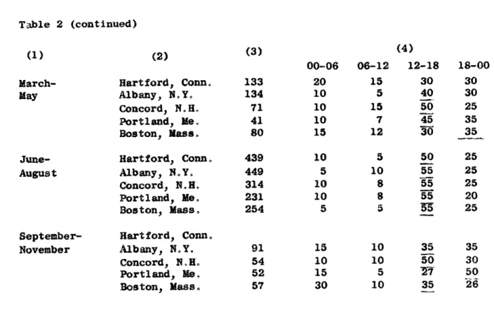
Table 2, "Diurnal variation of thunderstorm frequency", was obtained

from Hydrometeorological Report No. 5, Thunderstorm Rainfall, U.S. Weather Bureau. The stations in extreme southern New England are grouped together to show the affect of different regions. The table shows a pronounced max-imum of thunderstorm activity during daylight hours in the summer, particu-larly between the hours of 1200 and 1800 EST. In extreme southern New

England and its coastal waters, just as many thunderstorms occur during

nocturnal as in daylight hours during the spring and possibly fall.

The hail to _{thunderstorm ratio for New England, based on the years}

1904 to 1943 is 3 to 5%, with the maximum near and west of the Connecticut

River in southwestern Massachusetts and northwestern Connecticut

1. _{Provided by Mr. Lautzenheyer, U.S. Weather Bureau Climatologist,}

-11--Diurnal variation of thunderstorm frequency. (1906-1925)inclusive), After Hydrometeorological Report No. 5, USWB 1945.

Number

cases:

Percentage of time during hours:

00-06 06-12 12-18 18-00 December-February March-May June-August September-November December-February Nantucket, Mass. Block Island, R.I. New Haven, Conn. Providence, R.I. Nantucket, Mass. Block Island, R.I. New Haven, Conn. Providence, R

I,

R.I.

Boston,

Mass.

-12-Table 2 (continued) (1) March-May June-August September-November (2) Hartford, Conn. Albany, N.Y. Concord, N.H. Portland, Me. Boston, Mass. Hartford, Conn. Albany, N.Y. Concord, N.H. Portland, Me. Boston, Mass., Hartford, Conn. Albany, N.Y. Concord, N.H. Portland, Me. Boston, Mass.

Table 3, "Total number of hail days", shows a maximum of hailstorms in the interior regions of New England during the summer. Extreme southern New England and its coastal waters have maxima during the spring and fall months,

First order U. S. Weather Bureau station data in New England indicate only one to two hailstorm days per year. The author has seldom seen hail, and it was less than one quarter in diameter in the vicinity of Vineyard Sound and Buzzards Bay, Massachusetts. Hail occurred there only in cold, unstable air.

(3) 133 134 71 41 80 439 449 314 231 254 91 54 52 57 00-06 20 10 10 10 15 10 5 10 10 5 15 10 15 30 06-12 15 5 15 7 12 5 10 8 8 10 10 5 10 (4) 12-18 30 40 50 45 30 50 55 55 55 3 35 50 35 18-00 30 30 25 35 35 25 25 25 20 25 35 30 50 26

-13-T b1e

S

Station: No. of

Years: Jan: Feb: Mar: Apr: May: Jun: Jul: Aug: Sep: Oct: Nov: Dec:

Nantucket, 40 0 0 4 5 3 1 0 0 1 1 4 2 mass. Block Island, 40 0 1 5 5 2 2 1 3 2 1 4 1 R.I. Naragansett 14 5 6 6 7 0 1 1 0 1 0 1 6 Pier, R.I. Providence, 39 0 0 2 3 6 5 9 3 3 0 0 0 R.I. New Haven, 40 1 1 3 4 10 4 5 3 1 2 1 0 Conn. New York, 40 1 1 3 4 17 11 11 7 2 4 2 1 N,,Y. Boston, 40 0 0 1 3 5 5 8 3 1 0 2 0 Mass. Portland, 40 0 0 2 4 4 3 6 6 2 6 0 0 Me. Hartford, 39 0 0 2 5 11 12 15 7 1 1 2 1 Conn. Albany, 40 1 0 3 4 14 9 11 5 3 1 1 0 N Y. Burlington, 37 0 0 1 1 5 4 7 3 4 1 0 0 Vt., Northfield, 35 1 0 1 1 6 11 6 5 2 3 0 0 Vt0

Galway (1963) plotted 123 hail reports (see Fig. 4), in New England.for the period 1953 through 1962. He found a cluster of reports in north central Connecticut

approximately the tobacco growing belt, a crop which is quite susceptible to damage

by hail. Several reports of large hail were in east central Vermont, vn rrea which

was void of tornado reports. Severe weather reports clustered in the vicinity of the heavier populated areas (interior river valleys) and with the exception of north-eastern Massachusetts, away from the coastline.

-14-Insurance companies do not write a large amount of crop-hail insurance

in New England and consequently, the statistics would not provide an

Differences in rates have been made from statistics with a liberal

sprinkling of seasonal judgement.

Figure 5, "Areas with highest hail-crop insurance rates", shows the

areas where tobacco isggrown near Hartford, Connecticut and north of

Spring-field, Massachusetts.

The highest rates in Connecticut are on the east side

of the Connecticut River, indicated by "plus" signs while the rates are lower

The highest rates for general

crops in Massachusetts are for Berkshire,

Worcester and Middlesex Counties while in Vermont, Addison and Ruttand Counties have the highest rates.

C. Shorter period investigations.

As previously mentioned, most studies of thunderstorms in New England have been concerned with squall lines or cold fronts. In a study based on

synoptic data for four years, Penn (1955) found that 40% of New England squall

lines formed east of 75oW (Massena, New York to Philadelphia, Pennsylvania)

and 63% to the east of 80

W (Toronto, Ontario to Pittsburgh, Pennsylvania),

Swisher (1959) studied radar data of five squall lines in New England

and found the regions of development to be the Pocono Mountains in eastern

Pennsylvania and the Catskill Mountains of New York. Next came the Berkshire

Hills of western Massachusetts and the largest increase of development was in

the Connecticut River Valley. The squall lines decreased in intenity near

-15-the coast of Maine and in -15-the extreme sou-15-thern coastal areas of New England, where the bands dissipate. These results are in agreement with those of

Boucher (1958). Stem (1964) studied M.I.T, radar data during four days of air mass thunderstorms, near Boston, Massachusetts and found that these thunderstorms did not seem to form in a strictly random manner, There were preferred areas of formation, based on a combination of the low level con-vergence field (sea breeze effect) and local topography. He also observed that the air mass thunderstorms began to lose intensity on approaching the coast.

Some experienced forecasters, through personal communications, have provided the following observations regarding air mass thunderstorms.

Mr. Larry H. Shaw, Chief Forecaster at Westover Air Force Base, Chicopee Falls, Massachusetts said that air mass thunderstorms observed with the AN/CPS-9 radar, appear to have a preferred area for formation near Quabbin Reservoir, Massachusetts, perhaps on the west shore. This result agrees with observations made by Mr. Thomas Pisinski with the VISR-1 radar at Worcester, Massachusetts during the summers of 1960 through 1963.

Mr. Shaw noted another preferred area for formation in the northern Berkshire

Hills iind a few times that air mass thunderstorms formed about 15 miles

south-east of Westover Air Force Base, Massachusetts. Many of the thunderstorms moving into western and central Massachusetts formed in the Adirondack or Catskill Mountains of New York and moved eastward. They often dissipated before reaching the Connecticut River Valley, or shortly thereafter.

Mr. Robert L. Carlson, MIC at Green Airport, Hillegrove, Rhode Island,

northernRhode Island and their frequency is greater during the evening hours, Voyles and Zavos (1953) made a study of 1248 radar echoes of precipita-tion cells in New England moving from the southwest and which dissipated over water areas. The dissipations were 55% greater than would be expected under

a uniform distribution, particularly in the summer and autumn when the temper-ature contrasts between water and land diminish. Six hundred fifty one cells

which moved in any direction formed near the Connecticut River Valley north of Northampton, Massachusetts. Eighteen and seven tenth's per cent of all cells formed in this area, whereas uniform distribution would account for

3.6% The frequency is 415% greater than would be expected if the

distribu-tion were uniform.

Is-

-17-3, EFFECT OF TERRAIN ON AIRFLOW

A. Orographic and thermal effect.

There is a dynamical or orographic effect as the wind is forced to blow up a slope. This will start upcurrents and initiate the development of storms. A valley wind would enhance convective activity by carrying more moist air from low levels upward towards nearby hills or mountains

and the level of condensation would be lowered.

The thermal effect of terrain occurs when the slopes of hills or mountains are more perpendicular to the sun's rays than the valley floors, thus receiving more radiation per unit area. The slopes then are warmer than any horizontal surface and there is effectively a "high level" heat source. Streamlines would rise over the heat source and there is an

effective higher ridge.

B. Lee wave effect.

It was not until the 1940's that any serious study was made of mountain waves. Observational evidence was obtained in Europe by Forchtgott, Manley,

Kuetter, and others and later theoretical studies were developed that finally agreed with observations. The theory was mainly due to the works of Scorer

(1949, 1953, 1954, 1955) and Corby and Wallington (1956), in which a parameter

was related to the lapse rate and wind speed in the vertical. They found that lee waves were more likely to occur with an increase of wind with height and/or an increase of stability.

Berenger and Gerbier studied the effect of the size and shape of topo-graphy on lee waves in the French Alpes in 1956, 1957 and 1958.

-18-Davis and Booker (1962) studied the lee waves in the Alleghany Mountains of central Pennsylvania and related them to local formation and dissipation of unstable cloud systems. They found that lee waves were more likely to occur simultaneously with thunderstorms and theorized that outrush of cold low level air from a thunderstorm would enhance lee waves.

Cumulus growth would be discouraged in the descending part of the wave and growth might be enhanced in the rising portion, so that in some cases, the cloud would attain a sufficient buoyancy to survive the following descent. Thus waves could either encourage or discourage cumulus growth, depending upon timing of the growth with respect to the wave and the phasing of the waves with the terrain.

Figure 6, "Major terrain features near the watersheds of the ponds at Lakeville, Mass", shows minor ridges to the west and southwest of Copicut Hill,

about every five nautical miles. This hill has a theoretically ideal condition for thermals with a southwestward facing slope and a pronounced valley to the southwest. A southwest wind would then start thermals because of the orographic effect and the resulting clouds would not shield the slope from the sun.

One one occasion the author observed lee waves continuously forming cumulus congestus clouds about five miles east of the 354 foot Copicut Hill, They then moved eastward with the wind flow.

On 8 June 1965 from about 1330 to 1630 EST, the author observed a

cumulo-nimbus calvus cloud forming continuously to the lee of Copicut Hill. Individual cells were obscured by surrounding clouds and the radar data unfortunately were not available at this time. The author attempted to show that these air mass

0 sIDGI WArTI

tWoMSET

J

0

ISeUAnoS #AV

6

ALI

Fig.

6. Major

tertaia features near the

~20-thunderstorms were enhanced at the areas of maximum uplift by lee waves, but there was insufficient surface and radar data.

Mr. Miles Standish, State Conservation Officer confirmed that air mass

thunderstorms occur with an exceptionally high degree of frequency to the east of Copicut Hill, according to his observations of the past 15 years,

4. DATA AND METHOD OF ANALYSIS

A. Use of radar to locate thunderstorms.

The quantity measured by a radar when observing precipitation is the radar reflectivity per unit volume

Vk

1

I

region and Il=, (1) where = 0.93 for water perticles and

0.197 for ice particles.

The limits of the Rayleigh region are not precise, but depend on the degree of accuracy required. Actually it can usually be applied sE.tisfactorily

to particles considerably larger than but not as large as

When Z is obtained by applying equation (1) to measured ref~ectivities rather than from observed drop diameters, it is called equivalent Z and denoted

by Ze. When the conditions for Rayleigh scattering are fulfilled, Z and Ze are

the same within the limits of experimental error. For hailstones, the Rayleigh approximation is good within 2 db for diameters up to 3 cm when

X=

(Austin, 1962), but the suitability of using the relation for water particles depends upon the distribution of water and ice in the hailstones,

A criteria is now being sought for recognizing thunderstorm, using Ze

Donaldson (1961, 1965), Wilk (1961), Arnold (1961) and Hitschfeld and Douglas have made studies of the associated hail occurring with a given Ze using 3 cm

radar. These measurements are meaningful only if they are made at 20,000 feet

or higher, because of severe attenuation by water in the lower por%.ions of tho storms.

Geotis (1963) found with the 10.7 cm radar that when log Ze was greater than 5.5 near the ground, there was almost always hail in New England. The units for Ze are mm6 /m 3, but it is more convenient to use log units.

Ward (1965) used a 10 cm radar in Oklahoma and found that hail occurs occasionally with log Ze as low as 4.0, but the hail was usually not larger

than about 1/4 inch in diameter. Ninety per cent of the reported hailstorms

had cores with log Ze > 4.0, most of the storms with log Ze slightly less than 5.0 contained some significant hail, but the majority of hailstorms had

log Ze about 6.0. Log Ze was not often greatet than 6.0, even in severe

storms. These results agree with those of Geotis (1963) in Massachusetts.

In this study, a storm was considered to be a thunderstorm when log Ze 4.5, which was equivalent to 25 mm/hr of precipitation. A hailstorm was assumed when log Ze.> 5.5, equivalent to 100 mm/hr, as observed by Geotis

(1963). These log Ze criteria are somewhat arbitrary but appear to be

reasonable since they are based on the observations just described.

B. Radar data used in this study.

To determine when thunderstorms were observed by the MA.T. SCR-615-B radar, every PPI observation between March and October of the years 1958

through 1965 was examined to find storms with log Ze . 4.5. Intensity levels appear five db apart, a factor of three in reflectivity or two in equivalent

rainfall rate.

The SCR-615-B radar has a wavelength of 10.7 cm and a beam width of

of 95 miles, The elevation was usually set at one degree to get most of the power above the horizon. The range was usually set at 120 statute miles

and occasionally at 60 statute miles.

The PPI radar data are averaged, range normalized signal intensity contours, which can be interpreted as lines of equal Z values or of equal rainfall rate.

Every calibration and check were plotted to maintain the accuracy of Ze, Austin and Geotis (1960) have shown that when short period fluctuations are averaged electronically, and when the radar is carefully and freBquently calibrated, that measurements of radar reflectivity are accurate to about

2 db.

The M.I.T. radar is normally operated during the working hours 0800L to 1700L, Monday through Friday and after 1700L if the precipitation continues or is pretty clearly predicted. Nocturnal thunderstorms and weekend thunder-storms are often missed, Great emphasis was placed on squall line and frontal thunderstorms and some scattered air mass thunderstorms have been missed, The lack of nocturnal thunderstorm data can be a significant loss in and near

the coastal areas of southern New England in the spring and fall months. The author made a pilot study of every nocturnal thunderstorm from April 1958 to April 1960 that was observed by 1st order U.S. Weather Bureau and military

weather stations in southeastern New England. It revealed 37 thunderstorm days, and of these 28 were air mass thunderstorms, the remaining seven being associated with cold fronts. At least four of the days with air mass thunder-storms had troughs or closed lows near the 250 mb level, but not discernable at lower heights.

-24-C. Selection of air mass thunderstorms.

Thunderstorms are assumed to be of air mass origin when surface fronts are at least 200 miles away. Penn (1955) in a study covering four years of New England squall lines found that the distance between the cold front and squall line averaged 125 miles in the northern portion and 190 miles in the southern portion. A typical example of a day with air mass thunderstorms is a cold front in extreme western New York with scattered thunderstorms in

New England, If the cold front approached eastern New York, the thunderstorms in southeastern Vermont would not be considered as air mass type.

D. Method of analysis.

The PPI films were viewed through a modified TDC Mainliner number 200 projector and a Holmes number 3852 projector. Tracings were then made of

"levels" that correspond to log Ze N4.5 and log Ze> 5.5. There would be an

error in these tracings if in the process of photography, the scope was distorted or if there is a human tracing error when the image is projected,

Normally, a photograph was made of one level during each revolution of the antenna, This resulted in an average of about four minutes between successive photographs of the level corresponding to log Ze 4.5 or those

for log Ze> 5.5.

Since the air mass thunderstorms did not have an erratic behavior, it was easy to interpolate their areal coverage and time durations, even with time breaks, Tracing sheets had to be renewed about every 6C minutes of PPI data to simplify any analysis.

-25-The area swept within the radar range was divided into a grid of 100 square mile areas. Each area had coordina.es N, S for the north-south axis and W, E for the west-east axis, using M.I.T. for the origin. The frequencies of occurrence, formation and dissipation of thunderstorms for each of these areas were recorded as well as cell characteristics such as size and orienta-tion. If a cell extended more than three miles into an area from an adjacent area, it was considered as existing in both areas.

In order to find the effects of topography, a topographical barrier chart for southern New England was drawn. Then the pertinent 500-mb charts were examined for evidence of troughs and the general flow pattern, Since most of the topographical barriers in southern New England are orierted north northeast to south southwest, the 500-mb flow was grouped into the southwest, northwest, north and southbast sectors as well as a closed low or pronounced trough category. Then the formations, dissipations and durations of cells in each area were recorded for all these 500-mb flow patterns. Cell tracks were also drawn for each 500-mb flow pattern in order to determine their lengths and direction of movement.

All available National Meteorological Center synoptic and facsimile

charts were scanned to record general features and any parameters that indicate stability and moisture.

5. RESULTS

A. Number of days when thunderstorm echoes were observed.

As mentioned previously, the data consisted of radar records for the months March through October of the years 1958 through 1965,

All storms with log Ze 4.5 were considered to be thunderstorms and

all with log Ze> 5.5 were called hailstorms. There were 212 days when thunder-storms occurredSynoptic analysis indicated that on 148 days the thunderthunder-storms were not of the air mass type but were associated with the following large scale weather features. Cold fronts (70) and quasi stationary fronts (38) accompanied the majority of non-air mass thunderstorms. Warm fronts (21), occluded fronts (7), warm sectors (3), hurricanes or tropical storms (3) and cyclones (3) were responsible for the remaining cases. Appendices A and B give brief summaries of these synoptic features.

B, Characteristics of air mass thunderstorm days.

Days when air mass thunderstorms occurred were classified as to the 500-mb pattern. The direction of wind flow or the presence of closed lows

and/or deep troughs with wind direction shear were recorded. Since the major topographical barriers in New England are oriented in a north northeast to south southwest direction, the flow direction was classified as southwest, northwest, north, southeast and south southwest, as shown in Appendix B.

Out of 64 days with cells log Ze ,4.5, the flow was southwest to

west (clockwise) at 500 mb on 41 days, west northwest to north on 11 days,

a closed low or deep trough on eight days, south southwest flow on two days, southeast to south southeast flow on one day and north flow on one day,

On 38 out of 64 days, some cells had log Ze!5 5 The 500-mb flow was

souh-west to souh-west (clockwise) on 29 days, souh-west northsouh-west to north on six days and there was a closed 500-mb low or deep trough on three days.

The low level flow was examined by recording the 500 meter winds for Albany, NcY., J.F. Kennedy International Airport, N.Y., Nantucket, Massachu-, setts and Portland, Maine. On 40 out of the 64 days when storms with log Ze 4.5 were observed, there was confluence of the 500 m. wind flow at

either one or both of the southern radiosonde stations with respect to the northern ones,

The surface winds for the coastal or near coastal stations of Providence, R,&, Logan International Airport, Boston, Massachusetts and Portland, Maine were examined, and showed that 61 out of the 64 days had sea breezes, The Providence, R.I, surface winds would back and increase in speed, indicating a gradient induced sea breeze convergence line, This is similar to the circulations over the Brest peninsula of France and the peninsula of southern Ergland,

Appendix C, "List of days and their characteristics when the SCR-615-B radar recorded air mass cells with log Ze 4,45", gives a very brief descrip-tion of the synoptic situation, data obtained from the US. Weather Bureau

Local Climatological Data, Synoptic and Daily Weather Maps, National Meteor-ological Center facsimile charts and PPI radar data,

The Showalter index is used to indicate the stability and is computed

by lifting a parcel of air dry adiabatically from the 850 mb level until it

reaches saturation, assuming a constant mixing ratio. The saturated parcel

there with the actual 500-mb environment in OC is the index, It is best to use the Showalter index from the nearest radiosonde station in New England,

rather than to interpolatec The Showalter index and other parameters were obtained from available National Meteorological Center facsimile charts since 1962. The Showalter index was 4 +50C on all 35 days examined when log Zee 4.5 for the air mass cells.

The vertical velocity, w in cm/sec at 600 mb was 2 0 cm/sec on 20 out of 22 days examined when air mass cells with log Ze 4.5 were recorded,

The precipitable water is obtained by condensing out all the moisture in a vertical column from the surface to 500 mb, where most of the available moisture is, The precipitable water was greater than one half inch on all

39 days examined and 10 days had less than one inch.

The average relative humidity between 1000 mb and 500 mb was available on 15 days and exceeded 50% on all of them,

C. Characteristics of air mass cells,

A "cell" is defined for this study as the area enclosed by a contour "level" corresponding to log Ze = 4<5. This is then considered a

thunder-storm,

A total of 3878 individual cells were traced. The average daily number

of cells was 28 and that of hailstorms was five, The maximum number of cells

occurred on 10 July 1961 when there were 205 and 33 of these were hailsterns.

Cells vary in shape and sire during their lifetimes, so the ".verage"

cell size for each day was determined by inspection. This "average" cell size

-28-

-29-for each day is recorded in Appendix D and varied from 1 by 1 to 12 by 6 mdiles For all days, the average was 5 by 3J miles.

The largest cell measured 26 by 8 miles on 10 July 1961 and 20 by 10 mile cells occurred on 14 June 1963, 6 July 1964, 12 and 31 July 1962, 29 July

1963, 10 August 1960 and 31 August 1959. The number of days with cells having

one dimension greater than 10 miles was compfled for each l0xlO mile area, The number of cells per area ranged from 0 to 4 and minima for large cell

occurrences were in Maine and the coastal and sea areas off southern New England

Most cells were nearly circular but a few were very elongated, such as

the 20 by 5 mile cells on 19 July 1960 and 23 June 1965. The average

orienta-tion of the cell's major axis for each area is shown in F:.g. 7" Most of the cells had a north to south or north northeast to south southwest orientation of their axis. Beyond the 90 mile range, the axis became oriented perpendicular to the radar beam which is very evident to the north of M I..T in central New Hampshire. This indicates the beam filling effect, assum:ing that the cell's main axis actually remains oriented in a north northeast ;o south southwest

direction,, Most of the cells had an axis orientation within 40 from the average. These greater than 40 had a northwest to southeast orientation or

east to west orientation.

The quantitative analysis of cell duration was not made, but it was noted that small cells (2 by 2 miles) usually did not lasi. more than about

12 minutes, The cell heights recorded on the RHI of the AN/CPS-9 radar were available for 46 days. The average height of the cell tops was 34,000 feet and on three days they reached 50,000 feet, Stem (1964) analyzed RhI data of air mass cells and found that their life cycle was sim:.lar to one found

Fig. 7. Average orientations of air mass

cells with

leg

Z.

4.5 in

each

mile

square.

I I I I 8 -m

7

.2

.2

(

6

-2

*3

*3

w

5

o9

.3

S3

--

6

e

4

a

6

3

2

-13

.7

@3

e

.2

.2

z

10

20

30

40

50

6 0

70

-31-It was noted on many days that cell groups consisting of small cells

(2x2 miles) appeared to be equally spaced. Groups of larger cells (one axis.

5 miles) tended to be lined up rather than scattered about in a random fashion

The average distance between cell groups on 39 days was 30 miles. This agrees with Cochran (1961). The distance distributions are shown in Fig. 8, Any number to the right of the plotted data represents the number of occurrences.

There was a tendency for twice the individual day's average cell group distance when one or more cell groups were more distant from one another,

For example, on 19 July 1960, two cell groups were 55 miles apart while the remaining 13 were 25-35 miles apart; on 10 July 1961, two were 45 miles apart and 20 were 20 to 30 miles aparts; on 31 July 1962 two were 40 miles apart and five were 20 miles apart and on 25 July 1963, two cell groups were 70 miles apart while seven were 35 miles apart.

D, Cell motions,

The tracks of air mass cells were generally short (<15 miles), and usually corresponded to small cells with a short duration, Table 4 shows this distribution of cell track lengths. The four days that did not have any noticeable tracks had 500 mb lows or deep troughs. The longest cell

track was probably at least over 100 miles, partly in the radar shadow area on 9 June 1965. Other dates of long tracks were 23 June 1965, 14 August

1963, 12 September 1963, 31 May 1962, 12 July 1962. There were 17 days with

cell track lengths . 30 miles and 12 of these had cells with log Ze 5, 5,

All but one of the 17 days had cells with one dimension equal or greater

-32-Table 5 shows the distribution of 500 mb wind speed when long cell

tracks occurred. There were no wind speeds less than 20 kts.

Figure 9 shows the distribution of distances between cell tracks. Days with large distances had few tracks. When they were widely scattered, there was a tendency for distances to be in multiples of the average, 22 milesc On 31 July 1959, cell tracks were 25 and 45 miles apart.

Table 4. Length of cell track Length of cell Number of ce track (mi) tracks

1-5 698 6-10 549 11-15 150 16-20 124 21-25 44 26-30 36 31-35 24 36-40 14 41-45 8 46-50 10 51-55 5

Total number of tracks: 1679

Total number of tracks

<

s on 60 days. 11 Length of cell tracks (mi) 56-60 61-65 66-70 71-75 76-80 81-85 86-90 91-95 96-100 101-105 Number of cell tracks 4 5 2 1 3 0 1 0 0 1 : 1397

Table 5. Number of days with cell tracks greater than 30 miles and their

500 mb wind speeds.

500 mb wind (kts) Number of days

20 3 25 2 30 1 35 6 40 3 45 1 50 1

-38-30

20

10

0

FI

30

'

40

DISTANCE BETWEEN CELL TRACKS

50

60

(miles )

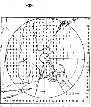
Fig. 10. Tracks of air mass cells with

leg

ze

4.5

which moved in different

directions *a 24 June 1959.

40

20

G. 9

70

-34-There is normally very little wind direction shear between 850 mb and 500 mb during days with air mass cells, except near a closed low or deep trough at 500 mb, This explains why the 500 mb flow was observed to be nearly parallel to the direction of cell motion, as shown in later figures of cell tracks,

Table 6 shows the distribution of wind direction shears (850 mb to

500 mb) on 24 days when air mass cells were near radiosonde stations, There

was usually a backing of winds with height and most wind shears were less than 20.

Table 6. Wind direction shears (850 mb to 500 mb) when air mass cells occurred,

Positive is backing and negative is veering with height. Total number of days was 24.

Wind shear (deg) Number of radiosonde reports

+400 1 +300 2 +20P 2 +100 7 0 9 -100 5 -200 0 -300 2 -400 1

On 18 July 1962 and 31 May 1962, the large intense cells moved at about

350 to the right of smaller cells, the latter moving parallel to the 500-mb

flowv, This movement is quite common with severe thunderstorms; Newton (1959).

On three days cells moved from the southwest to the northeast in southern

New England, whereas those in central New England moved from west to east, The dates were 12 July 1962, 11 August 1961 and 31 July 1959 and the phenomena

could be explained by a small backing of the upper level winds in southern New England,

On the afternoon of 24 July 1959, very unusual motion was observed-Cells with log Ze 4.5, measuring about six by five miles in horizontal

dimension, moved eastward with the 500-mb flow in southern Connecticut, while smaller cells (four by three miles) about 15 miles to the north moved north-eastward. Figure 10 shows tracings of the cell positions at about four minute intervals. The cells moved to the east in areas 5S, 10-5W and 6S, 9-8W

Other cells moved northeastward in areas 5S8W, 5S7W, 4S7W, 486W and 3S5W

The cells that moved eastward were in the Connecticut River Valley and just south of the 500 foot contoured plateau in southern Connecticut while those that moved northeastward started near Medhomasic Ht (800 feet) and were confined to the hilly plateau of eastern Connecticut,

Table 7 shows west southwest flow at station 74486, J0F. Kennedy

Inter-national Airport, N.Y., which is similar to the Albany, N.Y. and Nantucket, Mass, winds.

Fortunately some RHI observations were made with the AN/CPS-9 radar and they showed small turrets with tops to 40,000 feet and 45,000 feet of both cell groups that moved in different directions.

If field experiments near area 588W revealed complex lee waves with

intersecting maxima nodes extending in a southwest to northeast direction over the plateau, the different cell movements could be explained.

E. Detailed topography of area.

A topographical chart of southern New England showing the orientation

of the axis of pronounced ridges and mountains is in Fig. 11. It was construci.e

-36-areas where the mean elevation is less than 500 feet MSL, the mean 500 feet MSL contour and the most prominent hills and mountains with steep slopes

where the mean elevation is greater than 500 feet MSL. Some major features,

other than those previously mentioned, are the steep escarpments along the

east side of the Connecticut River Valley in Connecticut and Massachusetts, the plateau with elevation greater than 500 feet MSL in eastern Connecticut and western Rhode Island and minor hills such as the 350 feet Copicut Hill immediately east of Fall River, Massachusetts in area 5S1E. Table 8 lists a few areas with their topographical features that are referred to.

Table 7. Upper air winds on 24 July 1959 when cells moved in different directions near Middletown, Connecticut.

Station 74486 JFK

Wind directions are in degrees and wind speeds in m/ec

July 1959 Surface 150 m 300 m 500 m 1000 M 1500 m 2000 m 24/1200Z 240 03 242 08 246 11 258 13 261 12 248 12 240 l3 24/1800Z 240 06 241 07 242 09 243 10 250 11 251 12 248 1? 2500 M 3000 m 4000 m 5000 m 6000 n 7000 m 8000 T 24/1200q 239 13 242 14 255 17 260 19 269 17 261 19 250 12 24/180OZ 258 16 257 16 258 16 266 21 256 18 252 17 250 18 9000 m 1000 m 11000 m 12000 m 13000 m 14000 m 15000 m 24/1200Z 249 13 273 12 281 08 269 09 278 16 322 13 315 06 24/1800Z 249 15 250 13 251 15 251 16 253 17 264 15 290 05 16000 m 17000 m 18000 m 24/1200Z 304 05 026 02 029 03 24/1800Z 021 02 100 02 130 04

Some rivers are also shown, which are the long Conecticut River from

Long Island Sound northward through Connecticut and Massachusetts and forming

Fig. 11.

Map showing

tepographical

barrier, 500

ft

centour

and major

rivers and lakes (dotted

areas).