Diverging polygon-based modeling (DPBM)
of concentrated solar flux distributions
The MIT Faculty has made this article openly available.
Please share
how this access benefits you. Your story matters.
Citation
Loomis, James et al. “Diverging Polygon-Based Modeling (DPBM)
of Concentrated Solar Flux Distributions.” Solar Energy 122
(December 2015): 24–35 © 2015 Elsevier Ltd
As Published
http://dx.doi.org/10.1016/j.solener.2015.08.023
Publisher
Elsevier
Version
Author's final manuscript
Citable link
http://hdl.handle.net/1721.1/112643
Terms of Use
Creative Commons Attribution-NonCommercial-NoDerivs License
1
Diverging Polygon-Based Modeling (DPBM) of Concentrated Solar
Flux Distributions
James Loomis, Lee Weinstein, Svetlana V. Boriskina, Xiaopeng Huang,
Vazrik Chiloyan, and Gang Chen
1Department of Mechanical Engineering, Massachusetts Institute of Technology, Cambridge, Massachusetts, 02139, USA.
1 Correspondence should be addressed to G.C. ([email protected]).
ABSTRACT
This paper presents an efficient and robust methodology for modeling concentrated solar flux distributions. Compared to ray tracing methods, which provide high accuracy but can be computationally intensive, this approach makes a number of simplifying assumptions in order to reduce complexity by modeling incident and reflected flux as a series of simple geometric diverging polygons, then applying shading and blocking effects. A reduction in processing time (as compared to ray tracing) allows for evaluating and visualizing numerous combinations of engineering and operational variables (easily exceeding 106 unique iterations) to ascertain instantaneous, transient, and annual system performance. The method is demonstrated on a Linear Fresnel Reflector array and a number of variable iteration examples presented. While some precision is sacrificed for computational speed, flux distributions were compared to ray tracing (SolTrace) and average concentration ratio generally found to agree within ~3%. This method presents a quick and very flexible coarse adjust method for concentrated solar power (CSP) field design, and can be used to both rapidly gain an understanding of system performance as well as to narrow variable constraint windows for follow-on high accuracy system optimization.
KEYWORDS
Solar thermal energy; engineering mathematics; concentrated solar power; optimization methods
1. INTRODUCTION
We present a simple, purely geometric technique to rapidly assess flux distributions and performance characteristics of concentrated solar power (CSP) systems – such as lenses, heliostats (towers), linear Fresnel reflectors (LFRs), parabolic trough collectors (PTCs), and dish collectors. While best suited for LFR and heliostat arrays, with slight modifications this technique can also be applied towards PTC and dish collectors. Although PTCs are the most mature and widely used configuration worldwide (Barlev, et al., 2011), LFRs and heliostats are becoming attractive alternatives (Abbas, et al., 2012). For example, PTC technology accounted for about 490 MW out of 500 MW of operational utility-scale CSP as of January 2012 (Mendelsohn, et al., 2012). Looking forward, however, other configurations are gaining market share. For example, by 2015 there were greater than 450 MW of towers online with 1,600 MW of projects in development or under construction; and 170 MW of LFRs operational with 67 MW in development or under construction (SolarPACES, 2015). While not advocating for one type of configuration over another, simulation tools allowing for rapidly assessing and visualizing effects of
2
design variables and operational constraints will be a welcome addition for solar thermal energy utilization.
Concentrated solar power systems have a large number of design variables, which can be adjusted to optimize each system to respond to wide geographical variations in solar insolation and to customer specifications. This design space, coupled with large capital costs required for utility-scale deployment necessitates the use of accurate and robust numerical optimization tools. In particular, shading and blocking by adjacent mirrors and the receiver (Barlev, et al., 2011) are key considerations in array design and performance optimization in multi-reflector systems. While many simulation tools are available for the solar concentrator design, significant effort is typically required for specific project adaptation and implementation (Garcia, et al., 2008). The majority of existing codes are based on either ray tracing, for example SolTrace (Wendelin, 2003), MIRVAL (Ho, 2008), ASAP (Chen, et al., 2009); or convolution, such as RCELL (Lipps and Walzel, 1978), HELIOS (Biggs and Vittltoe, 1979), DELSOL (Kistler, 1986), and CIRCE (Ratzel and Boughton, 1987). The basis of ray tracing, which is a statistical Monte Carlo-based method, is to generate a random bundle of rays and individually track each ray’s progression from surface to surface. Each ray represents an infinitesimal bundle of photons, and the ray’s progress through the optical system is probabilistic. The irradiance of each surface is proportional to the number of impacting rays (Spencer and Murty, 1962). Numerical precision and calculation time scale with the number of rays and complexity of the system geometry (Garcia, et al., 2008). Advantages of ray tracing include greater flexibility and ability to model non-imaging optics (Garcia, et al., 2008). It is a time-consuming technique, however, which is poorly suited for use in optimization schemes and can require external determination of one-by-one mirror position and calculation of solar position.
The other popular tool in the solar concentrator modeling is convolution or cone optics. In convolution optics, rather than each ray representing an infinitesimal bundle of photons, rays originate from finite reflector sections. The spread of the rays is determined by convolving the designed distribution from the reflector section with Gaussian distributions corresponding to different system errors to give a more realistic distribution (Collado, et al., 1986). Convolution optics is therefore deterministic and models probabilistic processes through Gaussian error distributions. Convolution codes can achieve accurate performance with orders of magnitude fewer rays than ray tracing and are thus better suited for optimization. Convolution computational time scales with system geometry and number of convoluted integrals.
To design the optimal concentrator configuration, multi-parameter optimization is required to account for varying solar flux reaching the receiver; find the best system layout; and calculate instantaneous, transient, or seasonal/annual performance characteristics (Garcia, et al., 2008). This optimization underscores the need for the development of fast and flexible coarse adjust models that provide a preliminary system design by narrowing the range of design and operational variables. High-accuracy fine adjust numerical tools can then be implemented using this narrowed range of design constraints, yielding reduction in overall computational time and resources.
To this end, we developed an efficient computational method that reduces the modeling complexity of solar collector systems into its most fundamental elements. Unlike computationally intensive ray tracing, this method models the photon flux using purely geometric relationships implemented through a series of diverging polygon-based polyhedra. While less computationally expensive than ray tracing, in
3
convolution-based simulation methods errors can be pre-convolved to obtain a degraded sun shape (saving multiple convolutions) (Lipps and Walzel, 1978). Further study between optimized diverging polygon-based modeling (DPBM) code and convolutions is warranted; however, the authors believe that DPBM still presents an advantage as convolving functions is more computationally expensive than the simple geometric operations that are used for DPBM.
The major assumptions in DPBM include a pillbox sun shape, and that flux intensity along a given polyhedron surface (a single polygon) is constant within and equal to zero outside the bounds of the polygon. The pillbox sun shape also assumes a constant intensity along the solar disk and zero outside (Bule, et al., 2003) and is adequate for a large class of simulation problems (Sánchez and Romero, 2006). Given the high iteration coarse adjust goals of DPBM, its use is a reasonable assumption. While naturally this polygon assumption results in a loss of precision (and loss of edge effects), overall system performance was found to compare quite well with results obtained from ray tracing yet offering two orders of magnitude reduction in terms of computational intensity. As a coarse adjust method, a variety of system layouts and configurations can be quickly explored without need for complex simulation tools and provides the ability to quickly simulate and compare any number of different performance metrics of instantaneous, transient, or seasonal response (quickly exceeding 106 unique combinations of variables – where each ‘combination’ can be thought of as the equivalent to a complete stand-alone convolution or ray tracing simulation).
In this paper, we demonstrate the practical application of DPBM through design and analysis of an LFR array (using both planar and parabolic reflectors), and discuss how the model would be applied to a point concentrator (heliostat). In a linear concentration system, the polyhedral can be collapsed into 2D polygons, which for the purposes of this paper provides a clearer, more intuitive explanation than would be required for a point concentration configuration (such as a heliostat, which requires 3D polyhedron vertex calculations). Modifications to this model for other types of optics, receiver configurations, or reflector setup/geometry can be implemented by utilizing the same sequence of steps and methodology.
2. DIVERGING POLYGON-BASED MODELING (DPBM) DERIVATION
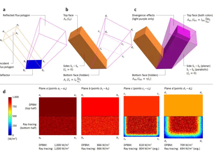
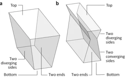
Figure 1 presents a summary illustration of DPBM. Starting with a reflector facet (Fig. 1a), an incident flux polyhedron is constructed such that its bottom polygon face is coincident to the reflector, the four polygon sides (S1 – S4) are parallel to the incoming flux, and the top polygon face is normal to this flux (Fig. 1b). Irradiance on the reflector is the incident flux (I0) times the ratio of top face divided by reflector area (𝐴0⁄𝐴1, which incorporates cosine losses). Setting the angle of incidence equal to the angle of reflection, a reflected flux polyhedron is constructed (Fig. 1c) such that the bottom polygon face is equal to the incident flux (not accounting for shading or blocking effects, which are discussed in detail later). Divergence in the reflected polyhedron is a combination of natural (solar divergence) and reflector properties (specularity error, shape error, surface slope error, etc.). Assuming no losses through the sides (𝐼𝑠= 0), and a pillbox sun shape, irradiance on any plane within the polyhedron is also given by the incident irradiance times the ratio of the surface areas (AR0/AR1). Figure 1d presents a sample comparison between flux profiles obtained from DPBM and ray tracing on four different polygon planes (normal to incident flux, reflector surface, and two planes within the reflected flux polyhedron). For any quadrilateral planar reflector, the incident and reflected flux polyhedra each have six polygon faces (top, bottom, two ends, and two diverging sides); likewise for a 4-sided parabolic trough reflector, the reflected flux
4
polyhedron has eight polygon faces (top, bottom, two ends, two converging sides, and two diverging sides, Fig. 2 shows. Theoretically, this technique could be extended to account for non-uniform cases by subdividing the polyhedron into smaller polygon elements within which the constant flux approximation can be used (subdividing would also be required to model single reflector geometries – such as PTC or dish). The linear DPBM assumption yields more conservative results than Gaussian because this linear assumption puts more flux towards the edge of the receiver, potentially missing the reflector. Ray tracing need not give a Gaussian distribution, but ray tracing tends to because in probability theory, given numerous independent random variables, their sum can be modeled as a Gaussian due to the central limit theorem.
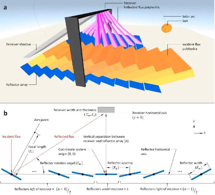
Regardless of array geometry, algorithm development follows five general steps – (1) reflector field/array setup; (2) incident flux polygon generation and shading; (3) reflected flux polygon generation and blocking, (4) performance characterization; and (5) variable iteration. An LFR array is used to demonstrate deployment of this algorithm (Fig. 3a).
2.1. REFLECTOR FIELD/ARRAY SETUP
First, based on design variables and system type, geometry of the reflector field and receiver is generated. The number of design parameters to use is adjustable: introducing more variables enables a larger degree of freedom in the simulation and more opportunity for optimization. For example in the LFR derivation presented in this paper, variables include reflector geometry (number, dimensions, spacing between adjacent facets, efficiency, divergence angle, and type, i.e., planar or parabolic); receiver geometry (dimensions, vertical distance from reflector field); and operational parameters (maximum acceptance angle of the receiver, minimum operational flux, system latitude/longitude/altitude, and day/time), Fig. 3b. A coordinate system is defined with the origin placed in a convenient location, such as the base of the receiver. Initial coordinates of each reflector (xz for LFR, xyz for heliostat), are calculated using design variables (reflector widths, lengths, layout, spacing, etc.). For simplicity in this demonstration, we set all reflector facets identical; however, as calculations for each reflector are conducted independently, this is not a requirement.
Once the basic array is set up, reflectors are rotated to simulate either single-axis or two-axis tracking (for LFR or heliostat configurations, respectively). Using algorithms adopted from National Renewable Energy Laboratory (NREL) guidance, solar zenith ( ) and azimuth ( ) are calculated based on simulated
position and time (Reda and Andreas, 2008). Next, a vector from the coordinate system origin to the sun is broken down into the angular components in the xz () and yz () planes (where the x axis corresponds to east–west and the y axis corresponds to north–south). Using Snell’s law, rotation angles are calculated such that a ray intersecting the center of each mirror’s center point would be reflected to intersect the receiver’s abscissa (Fig. 3b). For an LFR array, is used to calculate tracking angle for each mirror, and
used to apply a seasonal adjustment and adjust the incident irradiance (𝐼0) on each reflector element prior to introducing cosine losses from the rotational angle. Note that cosine losses due to are inherently
incorporated into the irradiance calculations (the ratio of the polygon surface areas, Figs. 4a, 4b), and do not need to be accounted for separately. For a heliostat, and are used for tracking calculations (Table 1 provides the associated equations). To enable performance assessment using both planar and curved (parabolic) reflector facets, reflector focal lengths (𝑓𝑖) are typically calculated for three different
5
cases –ideal, mean, and custom. While focal length for the curved reflector elements is calculated based on the vertical axis (following typical convention for a parabola) – in order to set a magnitude, we defined an ‘ideal’ focal length as the linear distance between the reflector and receiver abscissa if the reflector aim point was directed at the receiver abscissa. The ‘mean’ focal length, therefore, is merely the average of the ideal values for all reflectors, and ‘custom’ as a user-defined variable (thereby allowing for focal length optimization by scanning through a number of different values). The last item remaining in basic setup is to calculate associated slopes and line equations for each of the reflector elements, which are used in subsequent shading and blocking calculations.
2.2. INCIDENT FLUX POLYGONS
To generate incident flux polyhedra, polygon sides parallel to the incident solar flux vector are first created such that the entire reflector is covered (these serve as the foundation prior to any shading calculations, Fig. 4a). One of the disadvantages to LFR and heliostat arrays is that shading from both adjacent reflectors as well as the receiver can occur. Therefore, similar to the step described previously, a shadow polygon is calculated for each reflector and the receiver. For the receiver shadow, four cases are possible when evaluating each reflector – (1) incident flux to the reflector is completely shaded; (2) incident flux onto the reflector is partially shaded on one side, resulting in a single incident flux polygon; (3) incident flux onto the reflector is partially shaded, resulting in a split of the incident flux into two polygons – one on either side of the shadow; or (4) no shading. Based on which case exists, incident flux coordinates are modified. Likewise, if any reflector shadows happen to be shading incoming flux to a neighbor reflector, then its incident flux coordinates are similarly modified. After incident flux polygon shading effects are applied, assuming a pillbox sun shape, and zero loses through the sidewalls; cosine losses are incorporated where irradiance on the reflector (I1) is a function of initial solar irradiance (I0) and the surface areas of the top and bottom face (A0/A1). Note that solar divergence effects are not used in this step, only after the first intersection of flux with the reflectors. Because the incident and reflected flux in DPBM is broken down into simple geometric shapes, only coordinate vertices (indicated by circled numbers 1 – 4 on Fig. 3a) need to be tracked, a straightforward process in programs such as MATLAB.
2.3. REFLECTED FLUX POLYGONS
Reflected flux polyhedra are created using a similar approach as used for incident flux construction, as well as incorporating Snell’s Law, a solar divergence term, and a reflector divergence variable. Initial base vertices of each reflected flux polygon are created by setting them equal to the coordinates of the incident flux on each mirror – i.e., vertices of the bottom faces of the incident flux and reflected flux polygons are identical unless blocking occurs (or shading of the reflected flux, Fig 4b). As opposed to incident flux that experienced shading effects, blocking is any impingement to the reflected flux polygon prior to reaching the receiver. Blocking is accomplished via checking to see if any of the polygon sides intersect a neighboring reflector. If so, the polygon base area is reduced (by adjusting the appropriate vertices) in order to translate the offending reflected flux polygon side to be tangential to the neighboring reflector’s edge.
Divergence is taken into account in the reflected flux polygons by using a sun shape modeled in accordance with NREL’s best practices handbook, with a divergence angle (s) of 4.65 mrad (Stoffel, et al., 2010), a pillbox shape, and an average solar irradiance (I0) of 1,000 W/m2. Figure 4c shows these
6
divergence effects in a planar mirror, which result in irradiance always decreasing with increasing distance from the mirror. Stated another way, each reflected flux polygon carries some irradiance value with it, the magnitude of which diminishes based on distance from the reflector. Due to this effect, in large arrays as mirror distance from the receiver increases, divergence dominates and limits overall array performance. If a shaped (or parabolic) reflector facet is used, however, this effect can be mitigated. Figure 4d shows the divergence in a parabolic mirror, which can result in a much higher irradiance on the receiver. For simulating parabolic or shaped mirrors in DPBM, however, irradiance is first directly proportional to distance from the focal line (region i) then decreasing with distance from the focal line (region ii), as shown in Fig. 4d – meaning irradiance first increases as distance from the mirror increases, then after passing through a focal point, decreases as distance from the focal line increases (becomes more diverging).
Finally, after generation and modification of the reflected flux polygons, irradiance at the receiver is calculated by taking the ratio of the area of the polygon face incident to the receiver divided by the area of the reflected flux on the reflector. While they can be treated separately, in our simulation errors such as specularity error (sp), surface slope errors (surf), and shape error (sh) are grouped into a single total error term (r). The total error term is treated as an additional divergence contribution to the reflected flux by adding r to s.
2.4. PERFORMANCE CHARACTERIZATION
After application of all shading and blocking effects, individual irradiance contributions at the receiver from each reflector are summed and a number of performance metrics are investigated (Table 2). For example, maximum possible geometric concentration ratio (𝐶𝑚𝑎𝑥) is the ratio of the total ground area (𝐴𝑔𝑛𝑑) covered by the reflector field to the receiver area (𝐴𝑟𝑒𝑐𝑒𝑖𝑣𝑒𝑟). Irradiance received at the receiver (𝐼𝑅) is the integral of the flux over the receiver area. Conversely, actual concentration ratio (𝐶𝑎𝑐𝑡𝑢𝑎𝑙) is the mean flux at the receiver (𝐼̅𝑅) divided by the magnitude of initial irradiance (I0, or 1,000 W/m2). Therefore, optical efficiency was defined merely as the power incident to the absorber divided by the product of the incident flux to the ground area taken up by the reflector field (𝑜𝑝𝑡𝑖𝑐𝑎𝑙). However, the real array may be subject to operating constraints; therefore, a useful efficiency (𝑢𝑠𝑒𝑓𝑢𝑙) was defined as the average irradiance at the absorber subject to any operational constraints imposed on the model. Efficiency () includes cosine losses, shading losses, blocking losses, reflectivity, and various divergence angles. Finally, yearly array performance (Pyr) can be determined by integration of the receiver concentration ratio over the course of a year. Additionally, since vertices of all the array and flux components are known, a 3D figure can be displayed mimicking the simulated array. In MATLAB this can be accomplished with the 3D World Editor, a native virtual reality modeling language (VRML) editor.
2.5. VARIABLE ITERATION
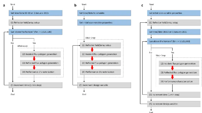
Finally, DPBM enables easy analysis of variable or operational constraint sensitivity. Using a series of nested loops, array performance can quickly be scanned with incremental adjustments to various parameters (such as design or operational variables). Figure 5a presents a simplified flowchart of scanning through an entire year in one minute time steps (5.3 × 10⁵ iterations). Similarly, other variables or combinations of variables can be changed to evaluate array performance. For example, Fig. 5b shows a
7
modified flowchart to examine a single variable, and Fig. 5c shows for a single variable and time. Further discussion is provided in Sections 3.2 and 3.3.
3. RESULTS
To determine the usefulness of DPBM, we first demonstrate accuracy of the method by comparing results from a number of array configurations with results obtained from ray tracing; second, we present several examples showing how DPBM can be used for analyzing design variables; and finally, we demonstrate use of DPBM for operational constraint analysis. For LFR arrays, typically planar solar receiver geometry is preferred (Mills and Morrison, 2000); therefore, we chose to use this configuration here.
3.1. RAY TRACING COMPARISON
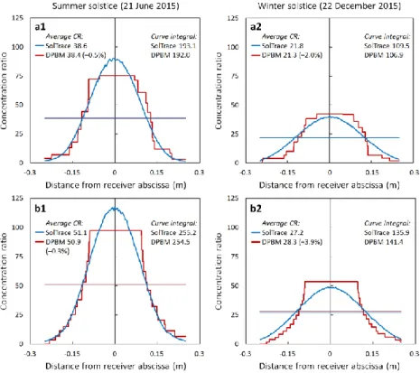
To evaluate simulation accuracy of our method, we compared solar flux distribution for two different LFR array geometries to results generated with NREL’s SolTrace (Wendelin, 2003), shown in Fig. 6. Geometries/configurations include 11 parabolic reflector elements with identical focal lengths (all f set to 18.6 m, Figs. a1 and a2); and 15 parabolic reflector elements with unique focal lengths (f ranges from 17.5 to 22.6 m, Figs. b1 and b2). Performance comparisons were simulated for both programs for noon on 21 June 2015 (summer solstice, ‘1’ plots) and 22 December 2015 (winter solstice, ‘2’ plots) for an array located in Phoenix, AZ. The plots show the concentration ratio incident to the receiver surface as a function of the receiver abscissa (all using identical 0.5 m wide receivers). Horizontal bars indicate the average concentration ratios obtained with each method (Table 3 provides simulation parameters).
Several items should be considered when evaluating these results. First, as compared to ray tracing, the homogeneous flux distribution, associated with the use of a pillbox sun, obtained from DPBM modeling results in underperformance near the center and over performance at the edges of a receiver. Therefore, one method to improve accuracy in system modeling is to ‘spot check’ DPBM results with a high accuracy method (such as ray tracing), and utilize this as feedback to adjust the reflector divergence variable. In this manner, one can account for the ‘smearing’ or loss of edge effects inherent to DPBM. For example in Fig. 7, the SolTrace modeling uses a surface slope error of 3 mrad (Gee, et al., 2010), for DPBM results shown the reflector divergence variable (represents a combination of specularity error, shape error, surface slope error, etc.) was set to 0 mrad. This value acts as a fitting parameter to represent a good compromise between the two methods. At the summer solstice, results for the concentration between the two methods agree within 0.5% and 0.3% for the 11 reflector and 15 reflector arrays, respectively. On the winter solstice, however, error between the two methods increases to 2% and 3.9%, respectively. Interestingly, when simulating these parabolic reflectors and adjusting the DPBM divergence variable to match ray tracing at the summer solstice, this adjustment resulted in discrepancies between the two methods – generally the lowest when irradiance was the highest (summer solstice), and highest when the irradiance was the lowest (winter solstice). This means that even though the discrepancy becomes larger when evaluating the winter months, when integrating the array performance over the course of a year – this effect is negligible effect since winter contributes a much smaller percentage to the total yearly array energy than summer. Clearly the polygonal assumptions used in our simulations result in a ‘stepped’ profile as compared to the Gaussian distribution obtained from ray tracing. As the number
8 of reflector elements (n) approaches infinity, lim
𝑛→∞(𝐷𝑃𝐵𝑀), however, the stepped profile results from DPBM will converge to a Gaussian distribution.
Overall, comparison of the two methods yields remarkable close results, considering the drastically reduced computational power required in our simulations and the ease of implementation and iteration. A rough simulation comparison (using geometry case A) between SolTrace and DPBM demonstrated a ~9 second runtime in SolTrace and ~1.5 × 10⁻² seconds in DPBM (~600× reduction, 1 × 10⁶ ray intersections). Nonetheless, several drawbacks to DPBM exist. First, this includes the time required to properly set up the initial model (true for ray tracing and convolution methods as well). The setup time is offset, however, by ability to quickly and automatically iterate all design variables once the initial model is completed. Second, analysis beyond optical performance, such as thermal cycles, is not considered. A further source of error is treatment of the modeling parameters as specific values rather than distributions that mirror inherent uncertainty in real-world systems (i.e., pillbox sun shape vice limb darkened sun); however, modifications can be made to suit particular project objectives. Detailed uncertainty analysis on the simulations is the subject of additional work; however, the greatest errors when predicting yearly CSP performance typically stem from non-optical components such as the turbine, thermal storage system, etc., (Garcia, et al., 2008). Additionally, one approach that could be used is to ‘spot check’ DPBM simulations with ray tracing results. For example – periodically using results from the high accuracy method (ray tracing) to tune the DPBM parameters (such as reflector efficiency, divergence, etc.) to minimize mismatch between the two methods, then continuing with the high iteration simulations. Certainly when conducting engineering analysis that requires highly accurate knowledge of temperature and flux distributions on the receiver, such as materials selection, one should periodically verify DPBM results with another method. These comparisons support the notion that using a simplified method, such as DPBM, is ideal for coarse adjust performance optimization.
3.2. DESIGN OPTIMIZATION
The ability to quickly run multiple types of simulations and generate copious performance metrics enables variable optimization. We demonstrate this by quantifying changes in system performance while iterating a single design variable ‘a’ (reflector width), a single design variable ‘b’ (focal length), iterating both design variables ‘a’ and ‘b’ simultaneously, and finally a time-dependent iteration of both design variables ‘a’ and ‘b’ (consisting of 150, 150, 5 × 10⁵, and 14.8 × 10⁶ iterations, respectively).
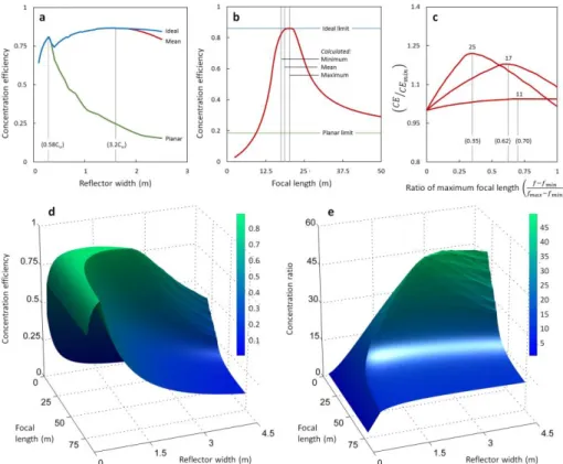
Figure 7a shows how concentration efficiency of the array changes as a function of reflector width for three different mirror cases – ideal (independent curvature for each mirror), mean (all mirrors identical), and planar mirror arrays (all mirrors identical planar curvature). Interestingly, efficiency was similar for all three cases up to reflector width ~0.6× receiver width – when planar efficiency drops drastically. This is due to the planar geometry resulting in larger amounts of flux missing the receiver. Conversely, since the parabolic mirrors account (at least somewhat) for effects due to solar divergence, efficiency remains fairly consistent until reflector width exceeds ~3× receiver width – when efficiency of the mean case starts to drop (due to skewing of the mean value from additional reflectors very far from the receiver). Figure 7b shows concentration efficiency as a function of focal length (all array mirrors identical). For comparison, the ideal focal length limit that represents a ‘best case scenario’, and the planar limit that is the concentration efficiency as f approaches infinity, are shown. This plot indicates that for the array
9
geometry shown, if using identical parabolic reflectors, the best choice focal length is not necessarily the mean value – somewhat counter intuitive. Rather, for this design geometry, the ideal value if all mirrors are identical is ~60% of the maximum. To reinforce that array performance is a function of all design parameters, and therefore must be simulated based on specific objectives for each project – Fig. 7c shows this peak f value as the number of mirrors in the array, and more significantly array width, changes. This plot suggests that as the total width of an LFR array increases, the optimal value of the focal length (at peak efficiency) shifts towards the minimum value of the (f – fmin)/(fmax – fmin) ratio, where fmin is the mirror-receiver distance for the central mirror.
Finally, we compared concentration efficiency as both variables, focal length and reflector width (Fig. 7d). When we scanned the performance as a function of the reflector width, the collector field dimensions change (the number of reflectors was kept constant). However, these changes in reflector field dimensions are accounted for in the efficiency and concentration ratio calculations. For comparison, Fig. 7e shows concentration ratio, rather than concentration efficiency for the same data. These two plots illustrate that different system geometries can yield vastly different performance relationships – for example, high efficiency and high concentration (medium width reflectors, short focal length); high efficiency and low concentration (narrow reflectors); low efficiency and high concentration (wide reflectors, short focal length); or low efficiency and low concentration (wide reflectors, long focal lengths). These intriguing results show just a few of the plethora of ways that a simplified model can be used to evaluate complex relationships between variables, and is a useful tool for simulating and visualizing these dependencies.
3.3. OPERATIONAL CONSTRAINTS
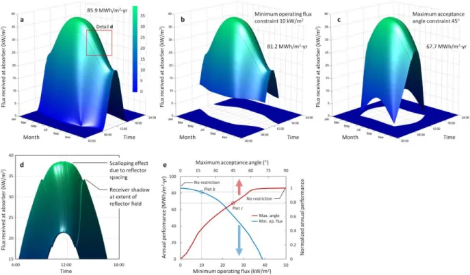
Because the main benefit of using a very simple model is ability to run a large number of iterations very quickly, various aspects of not only system design but also operational constraints over large time periods (i.e., annual) can easily be obtained. Similar to Garica et al, we generated a bi-directional solar field efficiency matrix (Garcia, et al., 2008), with ours providing solar field efficiency as a function of day and time. A surface plot of this data, Fig. 8a shows flux received at a receiver (geometry case A) from 0 to 24 hours each day between 1 January and 31 December 2015 (5.3 × 10⁵ simulations). Inset Fig. 8d shows the effect that the receiver shadow plays on array performance for this geometry – with a sharp decrease in flux as the shadow moves onto the array, and a scalloping effect as the shadow passes over the small spacing gap between reflectors. In this manner, the model provides a simple tool for visualizing annual performance, and potentially helps show otherwise hidden relationships. Flux at the receiver over the course of the year can be integrated to obtain total power for the design, as shown in Table 2. The ability to look at different performance aspects, apply various operational restrictions, and easily change/scan through various design parameters, makes such a method a powerful tool for ‘coarse adjust’ optimization.
(1) Minimum operational flux. The specific system may have operational constraints. For example, if a
minimum flux level is required to generate steam for turbines, then an operational constraint can be applied. Figure 8b presents one such scenario, clearly showing the loss in performance near sunrise and sunset each day due to flux <10 kW/m2 at the receiver.
(2) Maximum acceptance angle. Likewise, Fig. 8c presents a similar performance indicator, but with a maximum receiver acceptance angle vice minimum operational flux criteria applied. While relatively
10
(Cooper, et al., 2013). Interestingly, the loss in performance takes a different shape, with the bulk of loss occurring in the winter months (due to solar effects). Figure 8e shows a plot of actual and normalized annual performance of this particular array geometry as increasingly strict operational constraints are applied.
4. CONCLUSIONS
Here we presented development and analysis of a simple diverging polygon-based modeling method that can be used to evaluate instantaneous, transient, and annual flux distributions from a reflector field onto a receiver. While an ever increasing array of high accuracy tools become available, we believe that there is still a niche for a simplistic, easy to implement method capable of generating and visualizing complex relationships between the design and operational parameters.
The resulting simulation method was applied to an LFR array with a thorough step-by-step walkthrough provided. Based on a comparison between ray tracing method and our model, errors within a few percent were found. The low simulation time allows for numerous iterations of engineering and operational parameters to both gain a thorough understanding of array dependency on the variables, and also to provide a coarse adjust method to narrow constraints prior to a high accuracy (ray tracing or convolution) method of optimization. While the simulations here kept all mirror geometries identical, since parameters for all items are tracked independently, it would be trivial to incorporate effects of having different design geometries. For example – a combination of planar and parabolic geometries could be used in a single array, and the corresponding response evaluated. In closing, a DPBM approach provides a quick and flexible method useful for rapid assessment of CSP system performance due to changes in design variables or operational constraints, and can be useful for narrowing variable constraint windows prior to high accuracy system optimization.
ACKNOWLEDGEMENTS
This work was funded by Advanced Research Projects Agency – Energy (ARPA-E) under award number DE-AR0000471 for development of a Full Spectrum Stacked Solar-Thermal and PV Receiver.
AUTHOR CONTRIBUTIONS
J.L. and L.W. developed the models and wrote the manuscript. J.L. wrote the modeling software. X.H. assisted with SolTrace configuration. V. C. derived the angular projection for incident sunlight equations. All authors contributed to the concepts and discussions. G.C. directed the research.
COMPETING INTERESTS STATEMENT
11 REFERENCES
Abbas, R., Montes, M.J., Piera, M., Martínez-Val, J.M., 2012. Solar radiation concentration features in Linear Fresnel Reflector arrays. Energy Conversion and Management 54 (1), 133-144.
Barlev, D., Vidu, R., Stroeve, P., 2011. Innovation in concentrated solar power. Solar Energy Materials and Solar Cells 95 (10), 2703-2725.
Biggs, F., Vittltoe, C.N., 1979. The Helios Model for the Optical Behavior of Reflecting Solar Concentrators. Sandia Report SAND76-0347, 5-232.
Bule, D., Monger, A.G., Dey, C.J., 2003. Sunshape distributions for terrestrial solar simulations. Solar Energy 74 (2), 113-122.
Chen, C.-F., Lin, C.-H., Jan, H.-T., Yang, Y.-L., 2009. Design of a solar concentrator combining paraboloidal and hyperbolic mirrors using ray tracing method. Optics Communications 282 (3), 360-366.
Collado, F.J., Gómez, A., Turégano, J.A., 1986. An analytic function for the flux density due to sunlight reflected from a heliostat. Solar Energy 37 (3), 215-234.
Cooper, T., Ambrosetti, G., Pedretti, A., Steinfeld, A., 2013. Theory and design of line-to-point focus solar concentrators with tracking secondary optics. Applied Optics 52 (35), 8586-8616.
Garcia, P., Ferriere, A., Bezian, J.-J., 2008. Codes for solar flux calculation dedicated to central receiver system applications: A comparative review. Solar Energy 82 (3), 189-197.
Gee, R., Brost, R., Zhu, G., Jorgensen, G., 2010. An improved method for characterizing reflector specularity for parabolic trough concentrators, Proceedings of Solar PACES Conference Perpignan (France). 2124.
Ho, C.K., 2008. Software and Codes for Analysis of Concentrating Solar Power Technologies. Sandia Report SAND2008-8053, 1-35.
Kistler, B., 1986. A user’s manual for DELSOL3: a computer code for calculating the optical performace and optical system design for solar thermal central receiver plants. Sandia Report SAND86-8018, 5-148.
Lipps, F.W., Walzel, M.D., 1978. An analytic evaluation of the flux density due to sunlight reflected from a flat mirror having a polygonal boundary. Solar Energy 21 (2), 113-121.
Mendelsohn, M., Lowder, T., Canavan, B., 2012. Utility-Scale Concentrating Solar Power and Photovoltaics Projects: A Technology and Market Overview. NREL Report NREL/TP-6A20-51137, 1-55.
Mills, D.R., Morrison, G.L., 2000. Compact Linear Fresnel Reflector solar thermal powerplants. Solar Energy 68 (3), 263-283.
Ratzel, A., Boughton, B., 1987. CIRCE.001: A Computer Code for Analysis of Point-Focus Concentrators with Flat Targets. Sandia Report SAND86-1866, 1-53.
Reda, I., Andreas, A., 2008. Solar Position Algorithm for Solar Radiation Applications. NREL Report NREL/TP-560-34302, 1-16.
Sánchez, M., Romero, M., 2006. Methodology for generation of heliostat field layout in central receiver systems based on yearly normalized energy surfaces. Solar Energy 80 (7), 861-874.
SolarPACES. Concentrating Solar Power Projects http://www.nrel.gov/csp/solarpaces/ (accessed Aug 13, 2015).
Spencer, G.H., Murty, M.V.R.K., 1962. General Ray-Tracing Procedure. Journal of the Optical Society of America 52 (6), 672-676.
Stoffel, T., Renné, D., Myers, D., Wilcox, S., Sengupta, M., George, R., Turchi, C., 2010. Concentrating Solar Power: Best Practices Handbook for the Collection and Use of Solar Resource Data. NREL Report NREL/TP-550-47465, 1-129.
Wendelin, T., 2003. Soltrace: A new optical modeling tool for concentrating solar optics, 2003 International Solar Energy Conference, March 15, 2003 - March 18, 2003. 253-260.
12 FIGURES AND TABLES
FIG. 1. DPBM concept overview. (a) Relationship between sample reflector facet, incident, and reflected flux polyhedra. (b) Incident flux polyhedron detail and irradiance relationships – polygon sides parallel to incident flux vector, top polygon face normal to incident flux, and bottom polygon coincident with reflector. (c) Reflected flux polyhedron showing irradiance relationships and effects of polygon divergence. (d) Plots showing close agreement in sample flux comparisons between DPBM and ray tracing on planes a – d. Even with pillbox sun, however, with ray tracing you get penumbra effects due to sun's finite width.
13
FIG. 2. Number of polygon faces in a reflected flux polyhedron for (a) planer reflector and (b) parabolic reflector (degree of divergence exaggerated for clarity).
14
FIG. 3. Simulation overview. (a) 3D model of LFR array created using DPBM simulations. Array is generated to-scale based on user-supplied design variables. Axis of rotation is parallel to north-south vector, and array elements rotate east-west. Note that incident and reflected flux polyhedral arrays extend the full length of each reflector, but are shown truncated for clarity. (b) Initial array geometry is generated as a function of the design variables – shown for a single receiver LFR system.
15
FIG. 4. DPBM analysis on a 2D LFR setup. (a) Construction of incident flux polygons with shaded regions indicated. (b) Detail of blocking in reflected flux polygon. (c) Construction of reflected flux polygon using Snell’s Law plus divergence angles. (d) Reflected flux polygon construction using parabolic mirror.
16
FIG. 5. Sample algorithm iteration block diagrams for (a) Yearly performance simulation; (b) Single geometry (design variable) iteration; and (c) Combination of geometry and time iterations.
17
FIG. 6. Assorted comparisons between results obtained with DPBM and a widely used ray tracing program (SolTrace). Irradiance incident to the receiver as a result of: (a1, a2) LFR geometry case A (11 mean focal length reflectors); and (b1, b2) LFR geometry case B (15 ideal focal length reflectors). ‘1’ plots are simulated for noon on the summer solstice 2015, ‘2’ plots are noon on the winter solstice 2015. Phoenix AZ was used in all simulations.
18
FIG. 7. Design optimization example. (a) Concentration efficiency versus reflector width for ideal focal length, mean focal length, and planar focal length cases. (b) Evolution of concentration efficiency as a function of focal length (using a constant reflector width of 2 m). Ideal and planar limits are indicated, as are calculated minimum, mean, and maximum focal length values. (c) Normalized (both x and y axis) plot showing how optimal focal length (when all reflectors are identical) changes as a function of number of mirrors. Surface plots showing concentration efficiency (d) and concentration ratio (e) as a function of dual variables – reflector width, and focal length (generated from 2.5 × 10⁵ simulations, receiver shadow is turned off for clarity). Note that all are simulated for noon on an LFR array located in Phoenix, AZ on the summer solstice, and use geometry case A. The vertical distance between bottom of receiver and the reflector field is 17.5 m in all cases, other design parameters are listed in Table 3.
19
FIG. 8. Operational constraints overview. (a) Surface plot of flux received at the absorber (geometry case A) for calendar year 2015. (b), (c), Identical plot to (a) but with minimum operating flux of 10 kW/m2 (b) and maximum yz acceptance angle of 45 (c) restrictions applied. (d) Detail showing reduction in efficiency and scalloping effect resulting from absorber shading. (e) Actual and normalized annual as a function of operational constraint level. For surface plots (a) – (d), data points were simulated at one-minute time steps (5.3 × 10⁵ simulations per plot). All simulations conducted on array geometry case A located in Phoenix AZ.
20
TABLE 1. Solar position and breakdown into component angles. Quantity Symbol (units) Equation
Solar azimuth per NREL documentation (Reda and
Andreas, 2008)
Solar zenith 𝜃 per NREL documentation (Reda and
Andreas, 2008) Angular component in the xz plane 𝛼 𝑡𝑎𝑛 −1[𝑡𝑎𝑛(𝜃)𝑠𝑖𝑛()] Angular component in the yz plane 𝛽 𝑡𝑎𝑛 −1[𝑡𝑎𝑛(𝜃)𝑐𝑜𝑠()]
Direct normal irradiance (incorporating seasonal effects) on single-axis tracked system 𝐼1 (W/m2) 𝐼0 √sin2𝛼 + cos2𝛼 cos2𝛽 ⁄ ⁄ Horizontal irradiance 𝐼ℎ (W/m2) 𝐼0𝑐𝑜𝑠(𝜃) or 𝐼0 √tan2𝛼 + sec2𝛽 ⁄
TABLE 2. Sample performance metrics. Quantity Symbol (units) Equation Maximum possible geometric
concentration ratio 𝐶𝑚𝑎𝑥
𝐴𝑔𝑛𝑑
𝐴𝑟𝑒𝑐𝑒𝑖𝑣𝑒𝑟
⁄
Total irradiant power
at receiver 𝐼𝑅 (kW) ∬𝐴 𝐼𝑟𝑒𝑐𝑒𝑖𝑣𝑒𝑟𝑑𝐴 𝑟𝑒𝑐𝑒𝑖𝑣𝑒𝑟
Mean irradiance 𝐼̅𝑅 (kW/m2) 𝐼𝑅 𝐴 𝑟𝑒𝑐𝑒𝑖𝑣𝑒𝑟
⁄ Average concentration ratio 𝐶𝑎𝑐𝑡𝑢𝑎𝑙 𝐼̅𝑅 𝐼
0 ⁄ Optical efficiency 𝑜𝑝𝑡𝑖𝑐𝑎𝑙 𝐼𝑅 (𝐴𝑔𝑛𝑑𝐼0) ⁄ Useful efficiency 𝑢𝑠𝑒𝑓𝑢𝑙 𝐼̅𝑅(≥ 𝐼𝑚𝑖𝑛, ≤ 𝛿𝑚𝑎𝑥, 𝑒𝑡𝑐. ) (𝐴𝑔𝑛𝑑𝐼0)
Yearly performance (energy) 𝑃𝑦𝑟 (kW-h/m2-yr) ∫ 𝐼̅𝑅 𝑦𝑒𝑎𝑟
21
TABLE 3. Example LFR array geometry.
Case A Case B Case C
Number of reflectors 11 15 19 Reflector type Parabolic, mean focal length (all identical) Parabolic, ideal focal length (all unique) Planar (all identical) Reflector spacing 2.05 m Reflector width 2 m
Total collector width 22.5 m 30.7 m 38.9 m
Rim angle 32.7 41.3 48.0
Reflector length 50 m
Reflector focal length 18.6 m 17.5 – 22.6 m n/a
Reflector divergence angle 0
Reflector efficiency 0.95
Receiver width 0.5 m
Receiver length 50 m
Receiver thickness 0.5 m
Vertical distance between bottom