Distributed query execution on a replicated and partitioned database

Distributed Query Execution on a Replicated and

Partitioned Database

by

Neha Narula

B.A., Dartmouth College (2003)

MACHUSETTS INSTI OF TECH-NOLO'

nr-T i ;, ')nin

Submitted to the Department of Electrical Engineering and Computer

Science

in partial fulfillment of the requirements for the degree of

Master of Science in Computer Science and Engineering

at the

MASSACHUSETTS INSTITUTE OF TECHNOLOGY

ARCHNES

September 2010

@ Massachusetts Institute of Technology 2010. All rights reserved.

A uthor... ...

. ...

...

...

Department of Electrical Engineering and Computer Science

September 3, 2010

C ertified by ...

. ...

Robert T. Morris

Professor

Thesis Supervisor

Accepted by ...

Terry P. Orlando

Chair, Department Committee on Graduate Students

Distributed Query Execution on a Replicated and Partitioned

Database

by

Neha Narula

Submitted to the Department of Electrical Engineering and Computer Science on September 7, 2010, in partial fulfillment of the

requirements for the degree of

Master of Science in Computer Science and Engineering

Abstract

Web application developers partition and replicate their data amongst a set of SQL databases to achieve higher throughput. Given multiple copies of tables partioned different ways, developers must manually select different replicas in their application code. This work presents Dixie, a query planner and executor which automatically executes queries over replicas of partitioned data stored in a set of relational databases, and optimizes for high throughput. The challenge in choosing a good query plan lies in predicting query cost, which Dixie does by balancing row retrieval costs with the overhead of contacting many servers to execute a query.

For web workloads, per-query overhead in the servers is a large part of the overall cost of execution. Dixie's cost calculation tends to minimize the number of servers used to satisfy a query, which is essential for minimizing this query overhead and obtaining high throughput; this is in direct contrast to optimizers over large data sets that try to maximize parallelism by parallelizing the execution of a query over all the servers. Dixie automatically takes advantage of the addition or removal of replicas without requiring changes in the application code.

We show that Dixie sometimes chooses plans that existing parallel database query optimizers might not consider. For certain queries, Dixie chooses a plan that gives a 2.3x improvement in overall system throughput over a plan which does not take into account per-server query overhead costs. Using table replicas, Dixie provides a throughput improvement of 35% over a naive execution without replicas on an artificial workload generated by Pinax, an open source social web site.

Thesis Supervisor: Robert T. Morris Title: Professor

Contents

1 Introduction

2 Web Applications 2.1 Workloads ...

2.2 Partitioning and Replication 2.3 Development . . . .

2.4 Implications . . . .

3 Query Planning and Optimization

3.1 Query Plans . . . . ...

3.2 Choosing Plans to Maximize Throughput...

4 Design

4.1 Overview . . . . ... 4.2 Partitioning and Replication Schema . ... 4.3 Planner . . . . ... 4.3.1 Flattening . . . ... 4.3.2 Join Ordering . . . . ... 4.3.3 Assigning Replicas . . . ... 4.4 Optimizer . . . . ... 4.5 Executor . . . . ... 5 Implementation . . . . . . . . . . . . . . . . . . . . . . . . . . . . . . . . . . . . . . . . . . . . . . . . . . . .

6 Evaluation

6.1 Web Application Workload: Pinax 6.2 Setup . . . . 6.3 Query Overhead . . . . 6.4 Query Plans . . . . 6.5 Replicas . . . . 6.6 Comparison on a Realistic Workload

7 Related Work

7.1 Parallel Databases . . . .

7.2 Parallel Query Optimization . . . . 7.3 Partitioning . . . . 7.4 Key/Value Stores . . . .

8 Limitations and Future Work

9 Conclusion

List of Figures

1-1 Architecture for web applications . . .

3-1 Example Query 1 ...

3-2 Example Schema 1 . . . .

Architecture for Dixie . . . . Example Query 2 . . . . Cost Function . . . .

Microbenchmark 1 Database Schema Query overhead . . . . Microbenchmark 2 Database Schema Example Query 1 . . . . Measurement of Dixie's query plans .

. . . . 14 . . . 23 . . . 23 . . . . 30 . . . . 34 . . . . 38 . . . .. . . . 4 7 . . . .. . . . 4 8 . . . .. . . . 4 9 . . . .. . . .- 4 9 . . . .. . . . 5 0 . ... 51 4-1 4-2 4-3 6-1 6-2 6-3 6-4 6-5

List of Tables

3.1 Distributed query plans for Example Query 1 in Figure 3-1.. Estimated result counts for Query 1 . . . .

Row and server costs for Plan 1 . . . . Row and server costs for Plan 3 . . . .

Example AndSubPlan ... ...

Example AndSubPlan with Pushdown Join . . . Schema forfriends, profiles, and comments tables. A distributed query plan produced by Dixie... Distributed query plans, 1-2. . . . .

Distributed query plans, 3-4. . . . . Distributed query plans, 5-7. . . . . Estimated result counts for Example Query 2 . . . 4.9 Row and server costs per replica for different query plans.

Estimated result counts for Microbenchmark 1 . . . . Data for Microbenchmark 1 . . . . Additional Replicas . . . . Two different query plans . . . .

. . . . 32 . . . . 33 . . . 34 . . . . 34 . . . 35 . . . 36 . . . . 37 . . . . 38 . . . 39 . . . . 47 . . . . 48 . . . . 52 . . . 54 3.2 3.3 3.4 4.1 4.2 4.3 4.4 4.5 4.6 4.7 4.8 6.1 6.2 6.3 6.4

Acknowledgments

I am deeply indebted to my advisor, Robert Morris, who is a constant source of insight. His endless drive towards precision and clarity is helping me become a better writer and

researcher.

I consider it a privilege to work on the ninth floor with such inspiring people. Thanks to Nickolai Zeldovich for our fruitful discussions, and in general being a source of enthusiasm and an example of a prodigiously well-adjusted computer scientist. Thanks to Sam Madden and his students for almost all that I know about databases, and Szymon Jacubzak for the name Dixie.

My groupmates in PDOS created an environment where people are truly excited about systems; I owe a lot in particular to Austin Clements and Alex Pesterev for being easy to distract and for selflessly helping me administrate machines and solve technical issues.

Thanks to James Cowling for too many things to mention. I could not have done this without the advice and counseling of Ramesh Chandra, who gave me valuable insights on my own work methods, and helped me realize that none of us are in this alone. A huge thanks goes to Priya Gupta for ideas and feedback, and especially for being there to help me debug any problem, technical or otherwise.

Special thanks to all of my friends, east coast and west, for their encouragement and patience during this process.

And of course, this work would not have been possible without the love, support, and guidance of my sister, mother, and father, who instilled in me the intellectual curiosity and confidence to undertake research in the first place. Mom and Dad this is for you.

Chapter 1

Introduction

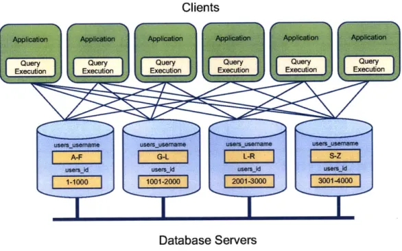
A common architecture for web applications is a relational database with a set of frontend web servers. Web application frontend servers are stateless, making it easy to add additional servers to handle more concurrent.user requests. As the traffic and number of frontend servers grow, the database server will become the bottleneck in the system. Partitioning a Web application's data across many database servers is a common way to increase performance.

Once a web application has partitioned its data, it can handle queries in parallel on multiple database servers and thus satisfy queries at a higher total rate. A horizontal

partitioning of a table is one that partitions a table by rows. Given a single copy of the data,

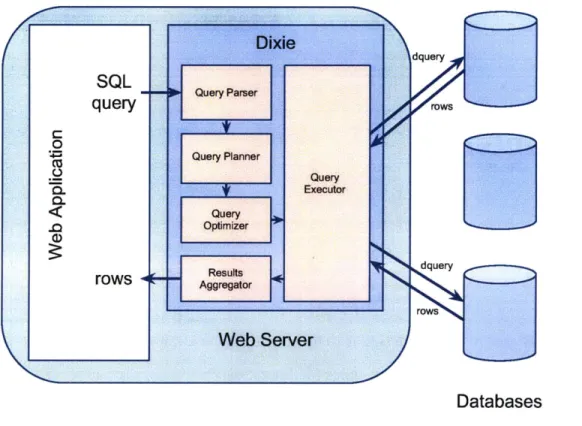
a table can only be horizontally partitioned one way, using one column or combination of columns as the partition key, assuming range or hash-based partitioning. The value of this column in the row determines which single storage server will store the row. Figure 1-1 shows a typical web application with a partitioned database.

Many workloads can benefit from more than one partitioning of the data. Suppose a web application issues two kinds of queries: those that can be addressed to a single database server to retrieve data, and those that must be sent to all servers. The system can execute more queries in the first category in parallel with the addition of more servers. Queries in the second will require the same percentage of overall storage server resources as more servers are added; dividing a query amongst N servers does not allow the system to process

N times as many queries per second. The reason for this is per-query overhead. Per-query overhead is the fixed part of the time to execute a query on a server, including time spent

Database Servers

Figure 1-1: Architecture for Web applications. Independent application webservers issue queries to a set of database servers. The users table is replicated and partitioned.

parsing the query and processing the request. If a query retrieves 100 rows, and those rows are spread out amongst N partitions, the application will have to send at least N requests. Suppose that per-server query overhead is 0. lms of CPU time. If a query has to go to all servers, the throughput of the system is bounded by a maximum of 10,000 queries per second regardless of how many servers are added. If a query can be satisfied on just one server, then query overhead would limit throughput to 10,000 qps on one server but only 100,000 qps on 10 servers. For small queries, per-query overhead is of the same order of magnitude as processing the whole query.

Our experience with web application data shows that there is rarely a single partitioning of a table that allows each read query to be directed to only one database server; web application workloads frequently contain queries that require data from multiple partitions or that cannot be addressed to a single partition because the query does not restrict to certain values for the partition key.

Replication addresses this problem by keeping copies of a table partitioned on different keys. A query can access the same data in a table using any replica. If the query's WHERE

clause restricts on certain tables and columns and there are replicas partitioned on those columns, then the query can often be sent to one partition instead of being set to N.

Using replicas, a developer can keep data partitioned in different ways so that more queries can be addressed to just one partition. However, having replicas of tables introduces the question of which replicas to use when planning the execution of a query. Each time a developer adds a replica of a table to improve the performance of a set of queries, she has to change every place in her code that might benefit from using that replica. In addition, choosing how to execute a query across such a partitioned and replicated database can be difficult. It requires a lot of effort on the part of the application developer to decide how to best execute queries.

This thesis presents Dixie, a query planner and executor for multiple shared-nothing databases tailored towards a Web application workload. Dixie runs on the client, intercepting SQL queries between a web application and the database servers shown in Figure 1-1, acting as the application's query executor. A query plan is a step-by-step execution plan for dividing a query over a set of database servers. To generate a single plan, the query planner chooses a replica for each table, an ordering of the tables for joins, and what work should be done in the server vs. the client. Dixie chooses good query execution plans by generating many query plans that use different replicas and different join orders and choosing the plan with the lowest predicted cost. Dixie computes a query plan's cost using a linear combination of the following two components:

e Total query overhead

- Total row-retrieval costs

Dixie estimates row-retrieval cost as the number of rows a server returns to the client. It models the entire query cost as a sum of query overhead for all servers with this row-retrieval cost, which is proportional to the total number of rows the client retrieves.

Dixie is novel because its cost formula recognizes that the cost of per-query overhead is significant enough to warrant choosing a plan which retrieves more rows but sends requests to fewer servers over a plan which retrieves fewer rows but sends a query to many servers; our experiments showed that the overhead of sending a query to a server was roughly

equivalent to retrieving 50 800 byte rows. This causes Dixie to choose some unexpected plans - for a join query which only returns one row, a plan which retrieves 50 rows into the client, 49 of them unnecessary, has higher throughput than a plan which only retrieves one row (see Chapter 6). Existing distributed query planners do not consider query overhead in this manner when choosing query plans.

This cost model omits the costs of both disk 1/0 and the time a database server spends processing rows that are never returned to the client. However, Section 6.3 shows evidence that this cost model is effective at predicting cost for the simple queries in our application workloads.

Dixie works by parsing application SQL queries and generating a sequence of backend server requests, different but also SQL, based on the data needed from each table. Dixie aggregates the results and does local SQL processing to return final results to the client. Dixie generates a plan per table replica per ordering of join tables, in addition to other plans detailed in Chapter 4.

The prototype of Dixie does not currently support writes. Dixie's design has two other major limitations. First, keeping many replicated tables increases the cost of writes because a row will be replicated amongst many servers. Second, Dixie has a different consistency model than that of a relational database - an in-progress read query will see the effects of concurrent writes, and for a window of time, a client might read stale data after reading a later version. Chapter 2 argues that web applications can tolerate this relaxed consistency.

This work makes two major contributions: First, a distributed query planner and executor which reduces the burden on application developers by automatically executing SQL queries designed for one database in a way that takes advantage of partitioning and replicas, without requiring any rewriting of application code. Second, a query optimizer which uses the observation that query overhead is a significant part of the cost of executing queries in a web application workload, and thus has a new cost estimation formula for distributed query plans.

We show that Dixie chooses higher throughput plans than a query optimizer that only considers per-row cost. Using Pinax [10], an open-source collection of social Django

applications, we also show that Dixie automatically takes advantage of additional replicas to improve overall throughput by 34% with no additional effort by the application developer. The rest of this thesis is structured as follows. Chapter 2 describes Web application requirements, workloads, and particular challenges in scaling, and Chapter 3 describes query planning. Chapter 4 describes Dixie's query planner, cost estimator, and executor. Chapter 5

details the choices and assumptions we made in implementing Dixie, and Chapter 6 shows how well it scales on queries and workloads relevant to Web applications. Chapter 7 discusses related work, Chapter 8 mentions limitations and directions for future research, and Chapter 9 concludes.

Chapter 2

Web Applications

This chapter describes characteristics of web application workloads which Dixie leverages for performance, and assumptions about what features are important to web developers. Specifically, it explains a web application's ability to do without transactions, how a web workload differs from traditional workloads described in previous research, and how those differences allow Dixie to make choices in execution.

2.1 Workloads

Web application workloads consist of queries generated by many different users, each accessing different but overlapping subsets of the data. A workload is a set of SQL queries along with a set of tables. Neither OLTP nor OLAP workload descriptions capture web application workloads, especially those of social applications. These workloads consist of queries which access small amounts of data, but will perform joins on multiple tables. The applications have both the goals of handling peak load and reducing query latency to

provide a real-time response to a user; system designers for OLTP traffic generally focus on throughput while those who work on larger warehouse-style databases optimize for latency.

Another feature of Web application workloads is that the database can satisfy most queries by using an index to retrieve rows from a table, instead of requiring a large scan to compute an aggregate. The entirety of the application's data is usually not large, and

this work assumes it will fit in memory. Finally, a user session usually consists of reading several web pages but only doing a few updates, resulting in mostly read operations.

2.2

Partitioning and Replication

We say a workload cleanly partitions if there exists a partition key for every table so that each query of the workload can be satisfied by sending the query to one server. For instance, given a workload for a link-sharing web site that supports comments, queries in the workload might look like the following:

SELECT * FROM links WHERE id = 3747; SELECT * FROM comments WHERE linkid = 3747;

A clean partioning would be to use l inks .id and comment s .linkid as the partition keys. However, if the developer changes the code to view comments by the user who wrote them, the workload will no longer cleanly partition, since one query needs to partition comment s by link-id and the other needs to partition by us ername.

SELECT *

FROM comments

WHERE username = 'Alice';

If the data is partitioned by something other than a column value, it might still be possible to find a clustered partitioning of the data so that all queries can be satisfied by the data on one machine, but the storage system would need to retain a reverse-index entry for every row in the table since a column of the row can no longer be used to determine the partition. Even with this relaxed definition, social website workloads in particular would rarely cleanly partition since users have overlapping sets of friends. Facebook considered a variety of data clustering algorithms to create isolated partitions and ultimately decided that the complexity was not worth the benefit [28].

Pinax's workload does not cleanly partition. 17% of all pinax queries use a table which another Pinax query refers to with a restriction on a different column. In order to address this

partitioning problem, web applications keep multiple copies of tables partitioned in different ways. In the example above, if the database also stored a copy of the comment s table partitioned by comments .username, the application could direct queries to retrieve a user's comments to that replica.

2.3 Development

Web applications are frequently built with frameworks like Django [3], CakePHP [2], Drupal [5], or Ruby on Rails [13]. These frameworks give the application an abstracted data layer which distances the developer from the actual SQL queries the application is making -she might never write a line of SQL. Frameworks typically generate queries that use only a small subset of SQL. In fact, Web applications don't need the full functionality of SQL; in our examination of Pinax and Pligg [11], an open sourced web application built to share and comment on links, neither used nested SELECT statements or joins on more than three tables.

It would be more convenient if developers did not have to modify their applications to use multiple partitioned tables. Web developers are generally not database administrators and would rather focus on developing application features instead of breaking through the application framework's data abstraction layers to rewrite their application for faster data access.

Web applications also seem to be able to forgo transactions. Django and Pligg by default use the MyISAM storage engine of MySQL [4], which does not provide transactions. Drupal used MyISAM as the default until recently (January 2010). Web application developers have already learned to build their applications to tolerate stale or slightly inconsistent data, by writing code to lazily do sanity checks, or by structuring their read-time code to ignore inconsistencies; for example when Pligg writes a link, it first inserts into the links table with a visibility status set to "off" until it has made changes to other tables, such as adding a new category or tag. It then returns and flips the status bit to "on". The application is written so that only "on" links are ever displayed to users.

2.4 Implications

These factors affect the choices made in Dixie's design, described in Chapter 4. Dixie focuses on choosing between multiple replicas of a table since web workloads do not cleanly partition, and Dixie does not support distributed transactions. Dixie supports a subset of SQL so that the application can continue to issue SQL queries. Since the important part of a web application's dataset fits in memory, Dixie does not consider the cost of disk seeks when choosing how to execute a query.

Chapter 3

Query Planning and Optimization

This chapter explains what is in a query plan and describes how to break down query execution into a set of steps. In addition, it explains how Dixie can estimate the costs of executing a query. The next chapter expounds on this by describing how Dixie generates plans and explaining Dixie's cost formula.

Query 1: Comments on Posts

SELECT *

blogpost, comments

WHERE blog-post.author = 'Bob' comments.user = 'Alice'

blogpost.id = comments.object

Figure 3-1: Comments Alice made on Bob's blog posts.

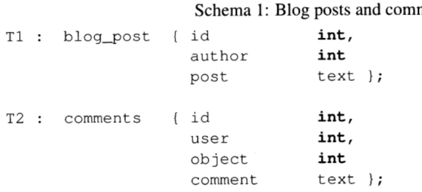
Schema 1: Blog posts and comments

Ti : blogpost T2 : comments id author post id user object comment int,

int

int

Figure 3-2: Schema for the blog post and comments tables.

FROM

AND AND

A query plan is a description of steps to take to execute a query. For each step, the plan contains a request for data, a replica for each table mentioned in the request, and a list of servers to which to send the request. For the purposes of this work, a replica is a range partitioning of a table amongst multiple servers using one column as the partioning key. Replicas are referred to by the table name and the column used to partition the table. In the application shown in Figure 1-1 in Chapter 1, the user s table has two replicas, one partitioned on us e rn ame and one partitioned on i d.

The query planner generates a plan for every combination of the following possibilities:

- Order of tables in the join

- Replica(s) to use to access each table

A join order is an ordering of tables which describes in which order to retrieve rows

from each table. Figure 3-1 shows an example Web application query which is referred to throughout the rest of this chapter, and Figure 3-2 shows the schema of each of the tables in the query. This query retrieves all of Bob's blog posts where Alice wrote a comment.

A predicate is a part of the WHERE clause of the form: Tablel.columnl = Table2.column2

The WHERE clause of a query consists of a set of predicates which must evaluate to true for every row returned. Each item in the predicate is an operator or an expression. An expression is either a table and column or a scalar value. A predicate can have multiple expressions or an operator other than equality, but for the purposes of this example we will only describe queries with an equality predicate and two expressions, either two tables with two columns or a table and column with a scalar value. A query that mentions multiple tables produces a join. A predicate that looks like Table1 .column1 = Table2 .column2 restricts the results of the join to rows with identical values in column1 and column2 of the two tables. The two columns are called join keys. A query can have more than two join keys.

The query in Figure 3-1 has three predicates, one of which contains the join keys. The join keys of this query are between blog-post .id and comments .object. Since it only accesses two tables, there are only two possibilities for join orders. Assume the

Ouer Stns Rplia Chice * blogpost author = 'Bob' Plan 1: SELECT FROM WHERE SELECT FROM WHERE

AND object IN ( B.id )

* comments user = 'Alice' * blogpost author = 'Bob' id IN ( C.object blog-post, comments comments.user = 'Alice' blog-post.author = 'Bob' blog-post.id = comments.object author,id user ,object user ,object author ,id blogs comments id & object

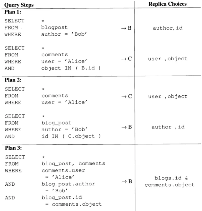
Table 3.1: Distributed query plans for Example Query 1 in Figure 3-1.

web developer has created the following table replicas: Two for the blog-post table partitioned on the id and aut hor columns and two for the comments table partitioned on the us e r and ob je ct columns.

* comments user = 'Alice' Plan 2: SELECT FROM WHERE SELECT FROM WHERE AND Plan 3: SELECT FROM WHERE AND AND Replica Choices Query Steps

3.1

Query Plans

Consider the plans shown in Table 3.1. Each plan has steps describing an execution strategy in the left-hand column, and a list of replicas available for each step in the right-hand column. Each plan is incomplete without a choice of replica. Dixie's backend servers understand SQL, so the request for each step uses a SQL query, referred to as a dquery. Each execution step also records how to store intermediate results. In later steps, each records how to substitute in previous saved results, described below.

Plan 1 describes an execution strategy where the executor first retrieves blog-post rows from the database servers using all predicates that apply only to the blog-pos t table, and stores the results in B, a temporary table in the database client. In the next step it retrieves all comments rows whose object column is the same as the id column in one of the blog-post rows retrieved in step one. The client sends a single dquery to each server including all the object values it needs in the list in the IN. As an example, if the results returned in step one have values (234, 7583, 4783, 2783) in the id column, the dquery in step two would be converted to the following:

WHERE comments.user = 'Alice'

AND comments.object IN (234, 7583, 4783, 2783)

Dixie's executor stores the results from the comment s table in C. At the end of the plan, the executor can combine the results in the subtables B and C by executing the original join over this data. It would execute Plan 2 similarly, except it retrieves comments first, then posts.

Plan 3 is a pushdown join. Pushdown joins are joins which are executed by sending a join dquery to each server so that the join can be executed on each database server, and the results aggregated in the client. A query planner can only create a pushdown join step if the replica of each table in the join is partitioned on the join key it uses with any other table in the join, otherwise only executing the join on each database server would produce incorrect results. Pushdown joins can have a lower cost if executing the join in two steps would require transferring large amounts of data back to the client.

Blog posts per author 10

Comments per user 50

Comments a specific user made on another specific user's blog post 1 Table 3.2: Average number of results

Blog Replica Comments Replica Rows Servers

id user 11 N+1

id object 11 N+n

author user 11 2

author object 11 l+n

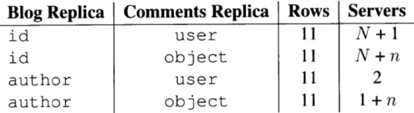
Table 3.3: Row and server costs per replica for Plan 1. N is the number of database servers, n is a subset < N.

3.2 Choosing Plans to Maximize Throughput

Which of these three plans is likely to yield the highest throughput? Dixie decides this by counting rows accessed and per-dquery server overhead. This makes sense because there is an overhead to retrieving a row, and there is an overhead to sending a request to an additional server, which is the cost of parsing the request and initializing threads to check for the data.

Using the statistics shown in Table 3.2 Dixie can estimate the number of rows returned at each step of the plan's execution. Given that there are ten blog posts per author, Dixie's query optimizer will estimate that a query which restricted on a specific author would return ten rows. Similarly, the optimizer would estimate a query which requested all the comments by a specific user to return 50 rows. For each step of a plan the combination of expressions in the predicates and choice of replicas determine to which servers a dquery is sent, and thus the query overhead cost. For example, using the blog-post .id replica in Step 1

of Plan 1 an executor would have to send a dquery to all N partitions, whereas using the

Blog Replica Comments Replica Rows Servers

id object 1 N

Table 3.4: Row and server costs per replica for Plan 3. N is the number of database servers, n is a subset < N.

IValueI Statistic

blog-post .author replica, it could send just one dquery to the partition with Bob's blog posts.

Tables 3.3 and 3.4 show the total estimated rows retrieved and servers contacted for execution of Plans 1 and 3, assuming N servers and considering different choices of replicas. Plan 1 will always retrieve 11 rows. No matter the choice of replicas the executor has to retrieve all of Bob's blog posts first, and then the one comment by Alice which is on one of those blogs.

Using the comment s .us er replica means that in the second step the executor could send a dquery to just the one server with Alice's comments. With the ob j e ct replica, the executor would have to send a dquery to whatever partitions were appropriate given the set of values returned as blog-post .id from the first step. We represent the size of this set as n, a subset of the N servers. The value of n could be 0 if no blog posts are returned from the first step, or N if the first step returns blog posts that have ids such that all the comments are on different partitions. Using replicas author and user, the number of servers contacted is 2.

Plan 3 always returns one row to the client, the row that is the final result of the query, though the database servers will have to read more than that in order to process the join. Based on row costs, a query optimizer should always choose Plan 3 when replicas

blog-post .id, blog-post .author, comments .user-id, and comments .object are available. Taking into account per-dquery server overhead costs shows that Plan 3 must send a request to every server, whereas Plan 1 will send dqueries to only 2 servers. Though Plan 1 fetches blog posts that Alice has not commented on into the client, on most systems the reduced query overhead makes Plan 1 a better choice. Chapter 6 shows measurements of overall throughput for Plans 1, 2, and 3 given varying amounts of data.

Chapter 4

Design

The main goal of Dixie's design is to maximize database throughput for web workloads by choosing a query plan that consumes the fewest database server resources. Dixie does this by generating plans and choosing replicas before calculating cost, and estimating which location would use the least amount of overall server resources. Note that this design goal is quite different than trying to minimize latency for a web application query, or trying to obtain maximal intra-query parallelism across many servers.

4.1 Overview

Figure 4-1 shows the architecture of Dixie. Starting with an input of a SQL query, Dixie parses the query and Dixie's planner generates a set of plans in three stages: first flattening the query tree, then splitting it up and generating subplans, and finally choosing replicas for each table access. Dixie's query optimizer evaluates the cost of each plan, chooses the plan with the minimum predicted cost, and sends this plan to the executor. Dixie's executor follows the plan by sending requests to a set of backend database servers, aggregating the retrieved rows, and returning the result to the application. Queries generated by the web application are queries and the requests generated by Dixie to the backend database servers

are dqueries.

Dixie focuses on queries that involve relatively small portions of tables so that straight-forward intra-query parallelization usually isn't useful, and the overhead portion of total

Databases

Figure 4-1: Architecture for Dixie. Dixie could run as a library inside the client or as standalone middleware.

query cost is significant. An OLAP-style query optimizer might optimize to send the query to replicas that maximize the number of partitions accessed, in order to parallelize data access. Dixie recognizes that in web application workloads, overall throughput does not benefit from intra-query parallelism. Instead, on these queries, Dixie chooses replicas and join orders to balance the number of servers accessed with rows read.

4.2 Partitioning and Replication Schema

The developer provides Dixie with a partitioning and replication schema. This schema should include a list of all replicas for each table, and the partitioning for each replica. A partitioning of a replica includes the partition key, which corresponds to a column of the replica's original table, and the range of the partition key present on each partition. Choosing an appropriate set of replicas and partitions for tables is important for good performance of a

---partitioned database, but is outside the scope of this work; Dixie requires that the developer establish a partitioning beforehand.

Dixie currently only works with tables that are fully replicated, in that all columns of a table are present in each replica. In order to save space, an extension of this work would be to consider tables that are only partially replicated, in that only a subset of columns or rows are part of a replica.

4.3 Planner

Dixie goes through three stages to generate a set of plans: flattening the WHERE predicate, creating different join orders, and assigning replicas. Dixie represents a plan as a set of ordered steps to pass to the executor. Algorithm 1 shows a template for a simple query plan. For each table t in the query, the planner creates a step which issues a dquery, DQt, and

saves the results in Rt both to fill in the next step's query and to compute the final result. The planner specifies which dqueries the executor should send in what order (or in parallel), what data the executor should save, how it should substitute data into the next query, and how to reconstruct the results at the end. Some plans will contain multiple loops that will be

executed in parallel.

Algorithm 1 A query plan represented as a sequence of steps. The executor will issue dquery DQt at each step and store the intermediate results in subtable Rt. The original query is applied to the subtables in line 4.

1: for all tables in Q do

2: Rt <- DQt(Rt_1)

3: end for

4: R <- Q(R1, R2, ..., RT)

5: return R

4.3.1 Flattening

Dixie first parses the application's SQL query into a query tree. The query's WHERE clause can have an arbitrary number of levels of nested ANDs and ORs. Dixie can execute a query with one OR by sending two dqueries and unioning the results in the client; it always

Table 4.1: Example An dSubP l an

executes an AND on one table by letting the database server execute the AND operation. Dixie needs to group ANDs and ORs appropriately, and to do so it needs to know which predicates apply to each table.

In order to fit the WHERE clause into a structure separating ORs and ANDs and filter predicates of a query to each step, Dixie flattens the the WHERE clause into disjunctive normal form, an OR of ANDs. As an example, consider the following clause:

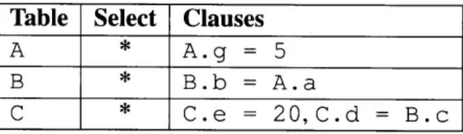
A.g=5 AND A.a=B.b AND B.c=C.d AND (C.e=20 OR C.e=4)

The planner would flatten this predicate as follows: (A.g = 5 A A.a = B.b A B.c =C.d A C.e = 20) (A.g = 5 A A.a = B.b A B.c= C.d A C.e = 4)

To create more plans, Dixie could also use conjunctive normal form or directly parse the WHERE predicate.

4.3.2 Join Ordering

Once the tree is flattened, the planner generates a set of AndSubPlans per AND clause. For instance in the above example it would generate a set of AndSubP lans for the clause

A.g = 5 A A.a = B.b A B.c = C.d A C.e = 4. An AndSubPlan consists of an ordering

of tables in the clause, the projection to retrieve from each table, and the predicates which are applicable to that table. The order of the tables in a join can greatly effect the overall number of rows retrieved, so it is important for Dixie to generate and evaluate plans with different join orderings. To generate an AndSubPlan, the planner considers all possible join orderings of tables in the corresponding AND clause. For the above example, the

planner would create the following set of table orderings: (ABC), (ACB), (BAC), (BCA), (CAB), (CBA)

Tables Select Clauses

A,B * A.g = 5,B.b A.a

C * C.e = 20,C.d =B.c

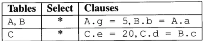
Table 4.2: Example AndSubPlan with Pushdown Join

This set represents the initial set of AndSubPlans for the first AND clause. For each table, the AndSubPlan includes the clauses specific to that table and the predicates that are dependent on a prior table in the subplan. Table 4.1 shows the AndSubP lan for the first ordering of tables. The planner generates additional AndSubP lans per AND clause to create plans for pushdown joins. Within an AndSubP lan, the planner combines each prefix of tables to create a join. For example, the planner would produce the AndSubP lan shown in Table 4.2. The planner creates each plan by choosing an AndSubP l an from each set in the OR, and produces a plan per combination of AndSubP lans.

plans = {AndSubPlanso X AndSubPlansi x ... x AndSubPlans}

4.3.3 Assigning Replicas

For each plan so far, the planner generates a new set of plans by creating a plan per combination of replicas for each table. It creates an execution step based on each step of an AndSubP lan. An execution step is a SQL query, a replica for each table in the query, and a set of partitions. The planner can narrow the set of partitions based on the replicas and expressions in each step; for example, in the plan where the planner used a replica of table A partitioned on A. g, the first step of the first AndSubP lan in Table 4.1 could send a dquery only to the partition where A. g = 5. The set of partitions for each step might be further narrowed in the executor. Each execution step also contains instructions on what column values from the results of the previous dqueries to substitute into this step's dqueries, by storing expressions which refer to another table. The substitution is done during execution. At this point Dixie has generated a set of plans exponential in the number of tables and replicas. In the applications we examined, no query has more than three tables and no workload required more than 4 replicas.. Thus the size of the set of plans generated was

Tabl RepicasAvaiabl friends: profiles: comments: {to-user, fromuser} {user, city}

{id, user, object, comment}

to-user, from-user user, city

user

Table 4.3: Schema for friends, profiles, and comments tables.

Query 2: Comments on Posts *

friends, comments, profiles

friends.from user = 'Alice'

profiles.city = 'Cambridge'

comments.user = friends.to user

friends.touser = profiles.user

Figure 4-2: Comments by Alice's friends in Cambridge.

manageable. For applications which wish to maintain more replicas or issue queries with many tables, Dixie would need to prune plans at different stages.

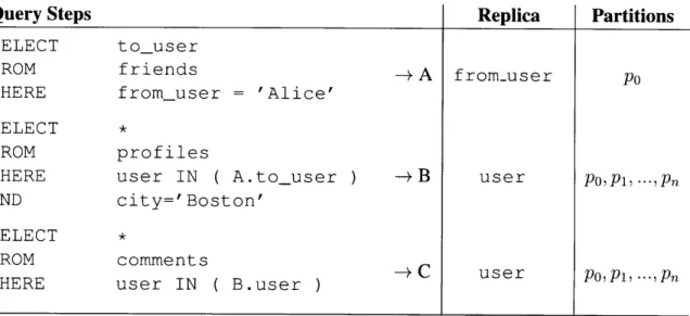
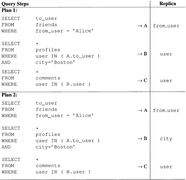
Table 4.4 shows a plan for the query shown in Figure 4-2, which retrieves comments made by all of Alice's friends in Cambridge using partitioned comment s, pro f ile s, and f r iends tables. The schema for the tables is detailed in Table 4.3.

to user friends

from user = 'Alice'

* profiles user IN ( A.to_user city='Boston' * comments user IN ( B.user Replica from-user user user Partitions Po poPi,...,Pn poPi,...,Pn

Table 4.4: A distributed query plan produced by Dixie.

SELECT FROM WHERE AND AND AND Query Steps SELECT FROM WHERE SELECT FROM WHERE AND SELECT FROM WHERE

Query Steps Replica Plan 1: SELECT FROM WHERE SELECT FROM WHERE AND SELECT FROM WHERE Plan 2: SELECT FROM WHERE SELECT FROM WHERE AND SELECT FROM WHERE -4 A I from.user to-user friends from-user = 'Alice' * profiles

user IN ( A.to user city='Boston' * comments user IN ( B.user to-user friends

from user = 'Alice'

* profiles user IN ( A.to-user city=' Boston' * comments user IN ( B.user A I from-user city user

Table 4.5: Distributed query plans, 1-2.

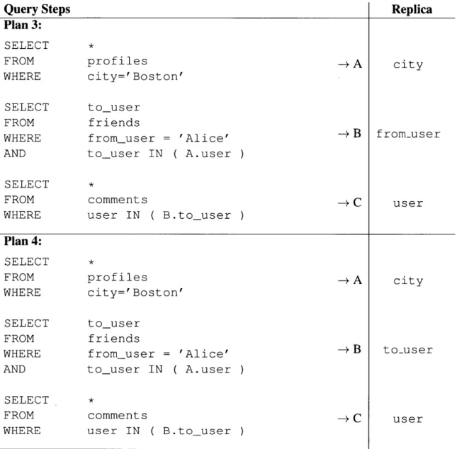
Tables 4.5, 4.6, and 4.7 detail different query plans Dixie's query planner would produce for the same query.

4.4 Optimizer

A cost model is a useful way to evaluate different plans. Once the planner generates a set of plans, Dixie's optimizer assigns a cost to each plan, and chooses the lowest cost plan for execution. Dixie models the cost by summing the query overhead and the row retrieval costs. Query overhead, cost,, is the cost of sending one dquery to one server. cost, is the

user

user Replica

Query

Plan 3:

SELECT *

FROM prof iles _{-+ A city}

WHERE city=' Boston'

SELECT to-user

FROM friends

WHERE from user = 'Alice' -B fromuser

AND touser IN ( A.user

SELECT *

FROM comments _{c user}

WHERE user IN ( B.touser

Plan 4:

SELECT *

FROM profiles _{- A city}

WHERE city=' Boston'

SELECT to-user

FROM friends

WHERE from user = 'Alice' 4B to-user

AND touser IN ( A.user

SELECT *

FROM comments _{c user}

WHERE user IN ( B.touser

Table 4.6: Distributed query plans, 3-4.

cost of data retrieval for one row, which includes reading data from memory and sending it over the network. Dixie's design assumes an in-memory working set and a set of indices to make the cost of retrieving any row roughly the same. Since all rows are in memory, row retrieval costs do not include the costs of disk 1/0. Dixie's optimizer computes costs using the following formula: the sum of the row retrieval cost per row times the number of rows retrieved and the cost of sending a query to a server times the number of dqueries sent.

cost = cost, * nr + cost, * n*

Quer Stes Relic Plan 5: SELECT FROM WHERE AND AND SELECT FROM WHERE Plan 6: SELECT FROM WHERE SELECT FROM WHERE AND AND * profiles, friends city='Boston'

from user = 'Alice'

profiles.user

= friends.to user

*

comments

user IN ( A.to user

*

profiles

city='Boston'

*

friends, comments from user = 'Alice' touser IN ( A.user comments.user = friends.to user + A I user, to-user user city to-user, user Plan 7: SELECT *

FROM friends, profiles, comments WHERE city='Boston'

AND from-user = 'Alice' to user,

AND friends.touser

_A

= profiles.user

AND friends.to user

comments.user

Table 4.7: Distributed query plans, 5-7.

Costs are only used to compare one plan against another, so Dixie's actual formula assumes cost, is 1 and scales cost,. Dixie uses table size and selectivity of the expressions in the query to estimate n,, which is based on the number of rows returned to the client, not the number of rows that might be read in the server. In addition to storing a schema for replication and partitioning, Dixie stores the number of rows in each table and the selectivity

Replica

Query

Statistic Estimate

Alice's friends 50

Profiles in Boston 500 Alice's friends in Boston 10 Comments by Alice's friends 200 Comments by Alice's friends in Boston 100

Table 4.8: Estimated row counts.

of each column, which is represented by the number of distinct keys in each column. It uses the cost function in Figure 4-3 to estimate n, the number of servers queried, and nr, the number of rows retrieved, both in one step. The selectivity function described in Figure 4-3 assumes a WHERE clause with only ANDs, so it can multiply the selectivity of the different columns mentioned in the query. This cost formula is simpler than that of a state-of-art

public int computeCost (QueryStep step) {

int numPartitions = step.partitions.size(; int numEstResults = 0;

for ( table : step.tables

double selectivity = table.selectivity(step.columns); numEstResults += table.tableSize * selectivity;

}

cost = scale(numEstResults) + numPartitions; return cost;

public double selectivity(String[] columns) { double selectivity = 1;

for ( col : columns) {

selectivity = selectivity * (1 / numDistinctKeys(col))

}

return selectivity;

Figure 4-3: Function to estimate the cost of a step in a query plan.

query optimizer. In future work Dixie should use dynamically updated selectivity statistics on combinations of tables. Table 4.4 shows the partitions and costs of each step of the plans shown in Tables 4.5, 4.6, and 4.7, using estimated row counts found in Table 4.8.

1 Po 50 1 Plan 1 2 PO, Pi, ,Pn 10 1

3 Po, Pi,., Pn 100 N 1 Po 50 1 Plan 2 2 Pi 10 1 3 PO, Pi, ... , Pn 100 N 1 Pi 500 1 Plan 3 2 Po 10 1 3 PO, Pi, ..., Pn 100 N 1 Pi 500 1

Plan 4 2 PO, Pi, ,Pn 10 N

3 Po, Pi,, Pn 100 N

Plan5 1 PO, P, Pn 10 N

2 PO, Pi, ,Pn 100 N

1 Pi 500 1

Plan6 2 Po, Pi, ,Pn 200 N

Plan 7 1 PO, Pi, ,Pn 100 N

Table 4.9: Row and server costs per replica for different query plans.

4.5

Executor

The executor takes a query plan as input and sends dqueries for each step in the plan to a set of backend database servers. The executor executes steps within an AndSubP lan in sequence, and executes each AndSubPlan in parallel. Dixie assumes that dqueries request small enough amounts of data that the executor can store all of the data from a step at once. The executor substitutes results to fill in the next step of the plan with values retrieved from the previous steps' dqueries.

The optimizer might assign a cost to a plan that is higher than the actual cost of execution. The executor can often reduce the number of dqueries it issues by further narrowing the set of servers required to satisfy a step's request. This means that the cost initially assigned to a step by the optimizer may not be correct. For example, in Plan 1, shown in Table 4.5, Alice's friends might all have similar user ids, and therefore will all be located on the same partition of the pro f ile . us e r replica. So in Step 2 of Plan 1, instead of sending a dquery to every server, the executor will only need to send one dquery to one server, reducing the query overhead and thus reducing the total cost. This might make this the best plan. The optimizer

has no way of knowing this at the time when it chooses a plan for execution, and so it might not select the optimal plan.

The executor uses an in-memory database to store the intermediate results and to combine them to return the final result to the client. This produces correct results because Dixie will always obtain a superset of the results required from a table in the join. As it executes dqueries, the executor populates subtables for every logical table in the dquery (not one per replica). After completion, it uses the in-memory database to execute the original query on the subtables and return the results to the client.

Chapter

5

Implementation

We have a prototype of Dixie written in Java which runs against a set of MySQL databases. We made several choices in building the pieces of Dixie's implementation - the subset of SQL Dixie handles, the query parser and database client, and the database system used for the backend servers.

The prototype of Dixie uses an off the shelf parser, JSQLParser [7], to create an interme-diate representation of a SQL query. Since JSQLParser does not handle the full syntax of SQL produced by Django, we altered JSQLParser to handle IN queries and modified some of Django's queries to convert INNER JOIN queries into join queries which use commas, as shown below. These queries are equivalent in MySQL.

SELECT *

FROM profiles

INNER JOIN auth user

ON (profiles.userid = authuser.id)

WHERE profiles-profile.location = 'Boston'

SELECT *

FROM profiles, auth-user

WHERE profiles.userid = authuser.id

It is much simpler for Dixie to execute dqueries in SQL instead of inventing a different intermediate language. We chose MySQL, a popular open source relational database, as the database backend. We tested the effectiveness of Dixie using queries generated by applications from Pinax, an open source suite of social web applications including profiles, friends, blogs, microblogging, comments, and bookmarks. Pinax runs on Django, a popular web application framework.

Dixie is written in Java, so it sits as a middleware layer between clients running Django and the MySQL database servers. It accepts SQL query strings and returns results in the Java Re sult Set format. In order to sanity check Dixie's results on multiple databases, we issued the same set of queries to Dixie using a partitioned set of replicas on four databases and to a single database server containing the same data but with only a single replica per table. We compared row-by-row results returned by both.

Dixie keeps static counts of number of rows, partitioning plans, replicas, and distinct key counts for each table. These are stored in YAML configuration files which are read on start up and not updated. Implementing a mechanism for updating these configuration files on the fly as replicas are added and deleted or as table counts change is left as future work.

Dixie executes plans by executing each execution step sequentially, sending the step's dquery to each partition's MySQL server listed in the step. This could be done in parallel to speed up latency of the query, but it doesn't affect the throughput measurements since every experiment runs many concurrent clients. Dixie saves intermediate results in an in-memory database, HSQLDB [6]. Dixie then executes the original query against this in-memory database, and returns a Java Re sult Set. An alternative implementation would have been to construct the response on the fly as results are returned from each partition and each step, but using an in-memory database allowed us to handle a useful subset of SQL without having to write optmized code to iterate over and reconstruct results. The Dixie database client uses JDBC to execute requests to the in-memory and MySQL databases.

Chapter 6

Evaluation

This chapter first measures and explains an example query where Dixie achieves higher throughput than an optimizer whose goal is intra-query parallelism, and then compares their performance on a full Pinax workload. Our sole measurement of performance is overall throughput of the system, measured in application queries per second with many concurrent clients.

6.1

Web Application Workload: Pinax

We use the social networking application Pinax to evaluate Dixie's performance. Pinax is built using the web application framework Django, and is a suite of various applications found in a typical social website. All queries in the workloads in Sections 6.4, 6.5, and 6.6 are directly generated by Pinax, and the queries used in the microbenchmark are derived as additional functionality from Pinax's schema. In this evaluation we focus on the profile, blog, comment, and friend features of Pinax. Each user has a profile page, and each user can add friends in a one-way relationship. The workload is made up in equal parts of viewing profile pages, viewing friends' blogs, and viewing comments. We used Django's client framework to generate SQL traces of application queries as though a user were browsing the site. Unless stated otherwise, each experiment uses these traces. We refer to this workload as the macro Pinax workload.

In addition, we conducted some experiments against a narrowed Pinax workload. In this workload, we removed queries of the form:

SELECT *

FROM auth user

WHERE auth user.id = 3747

This is a very frequent query that Django's auth system issues. In all experiments, both executors will send this query to one partition using the replica of aut h-us e r partitioned

on id.

There are 1.2 million users, 1.2 million profiles, 2.4 million blog posts, 12.2 million comments, and 5.7 million friendships in the database tables. The workload consists of many sessions with seven different start page views, and then a variable number of pages viewed depending on how many friends a user has. Each session is conducted with a randomly chosen logged-in user.

Pinax produces some SQL queries which when executed on a large database take a prohibitively long time, and skew the measurement of throughput. As an example, Django creates the following query when viewing the All Blog Posts page:

SELECT *

FROM blog-post

INNER JOIN auth user

ON (blog-post.authorid = authuser.id)

WHERE blog-post.status = 2

ORDER BY blog-post.publish DESC

This query requests the entire blog.po s t table joined with the entire auth-user table into the client. Even adding a limit causes MySQL to perform a scan and sort of the entire blogpo st table, which in these experiments was 2.4 million rows, with an average row length of 586 bytes (1.3 GB). In order to speed up the performance of this query, which is unlikely for a web application to ever issue to respond to a real time user request, we added a LIMIT, an index on blog.post .publish, and a signifier to indicate to MySQL the

order to join the tables. This reduced the time of the query from 7 minutes to .07 seconds. The following is the modified application query:

SELECT STRAIGHTJOIN *

FROM blog-post, authuser

WHERE blog-post.authorid = authuser.id

AND blog-post.status = 2

ORDER BY blog-post.publish

DESC

LIMIT 20

6.2 Setup

Evaluation Hardware. Each database server is a Dell PowerEdge 850 with a single Intel Pentium(R) D 2.80GHz CPU and 1GB of RAM. We run four database servers in all of the following experiments, unless specifically noted otherwise. We use three client machines, each with 8-16 cores running at 2.80 to 3.07GHz, and a range of 8GB to 12GB of memory. In all experiments, the throughput is limited by the database servers.

MySQL Configuration. Each database server is running MySQL 5.1.44 on GNU/Linux, and all data is stored using the InnoDB storage engine. MySQL is set up with a query cache of 50 MB, 8 threads, and a 700 MB InnoDB buffer pool.

Measuring Throughput. First we run Dixie's planner and optimizer on traces of application queries to generate traces of plans. During every experiment, each client machine runs a single Java process with a varying number of threads. Each thread opens a TCP connection to each database server, and reads pre-generated plans one by one from its own trace file. It runs Dixie's executor to perform the dqueries and post-processing in each plan, and then goes on to the next pre-generated plan. We pre-generate plans in order to reduce the client resources needed at experiment time to saturate the database servers. On this workload, generating a set of plans and running the optimizer to calculate costs took an average of 1. 14ms per query.

Throughput is measured as the total number of queries per second completed by all clients for a time period of 30 seconds, beginning 10 seconds after each client has started, and ending 10 seconds before the last client stops. We vary the number of threads per client until we produce the maximum throughput, and then use the average of 3 runs. Before measurement, each experiment is run with a prefix of the trace files used during the experiment to warm up the operating system file cache, so that during the experiment's three runs the databases do not use the disk.

Comparison. In all examples, we compare Dixie to a query optimizer which works exactly like Dixie except that that the competing optimizer does not take the number of

servers accessed into account when computing the cost of a plan.

6.3 Query Overhead

This experiment derives a value for query overhead by graphing the time per query varying the number of rows per query. This motivates the work in this thesis by showing that for small queries which retrieve fewer than 100 rows, query overhead is a significant part of the cost of issuing a query.

To measure the effect of query overhead, we run a single MySQL 5.1.44 server with one table of 1,000,000 rows of seven 256 character columns, described in Figure 6-1. Each column has a different number of distinct keys shown in Table 6.1, and as such a different number of rows returned when querying on that column. Figure 6-2 shows the time per query measured as 1/qps where qps is the throughput in queries per second, as a function of the number of rows returned by the query. The number of rows retrieved by each query is varied per run by changing the column in the query. Throughput is measured by running 8 client threads on one machine, each generating and issuing queries of the form:

SELECT cl,c2,c3,c4,c5,c6,c7 FROM test1

WHERE c5 = 2857

Within a run each client thread issues a sequence of queries requesting a random existing value from that column. The client saturates the CPU of the database server. The overall

TABLE testl: (cl varchar(256), c2 varchar(256), c3 varchar(256), c4 varchar(256), c5 varchar(256), c6 varchar(256), c7 varchar(256));

Figure 6-1: Schema for query overhead measurement benchmark

Column Distinct Keys Average Rows Returned

cl 500000 2 c2 250000 4 c3 100000 8 c4 40000 23 c5 20000 46 c6 10000 115 c7 4000 230

Table 6.1: Distinct key counts per columns

throughput of a run as measured in queries per second is a sum of each client thread's throughput, measured as a sum of queries issued divided by the number of seconds in the run. The queries per second measurement is converted to a milliseconds per query measurement by dividing 1000 by the total throughput.

Figure 6-2 is a graph showing how query processing time increases as the number of rows retrieved increases. This line is represented by the formula tq = to + x * tr, where tq is the total time of the query, t, is query overhead, x is the number of rows retrieved per query, and t, is the time to retrieve one row. The y-intercept of the line represents query overhead, and the slope of the line is the cost of retrieving one row. Using the data in Table 6.2, on our experimental setup we measure query overhead as 0. 14ms and the time to retrieve one row as 0.013ms. This means that retrieving 10 rows from one server takes .27ms, and retrieving 10 rows from two servers takes .41ms, a 52% increase in time. Retrieving 100 rows from two servers instead of one server results in a 10% increase in time.

Based on this experiment, our prototype implementation of Dixie uses values of 1 for

3.5 3 2.5

a

Figure 6-2: Measurement of milliseconds spent executing a query on a single server database, varying the number of rows per query using multiple clients.

Rows per Query Queries/sec

2 5925 4 4889 8 3764 23 2231 46 1340 115 612 230 306

Table 6.2: Throughput in queries per second varying the number of rows retrieved per query.

6.4 Query Plans

This section compares the performance of the three plans described in Table 3.1. Chapter 3 explained how Dixie would execute the query show in Figure 6-4. This section shows that Dixie chooses the highest throughput plan by using a cost formula which includes per-query overhead.

If a planner and optimizer were to just consider row retrieval cost, it would select Plan 3 in Table 3.1 since it retrieves the fewest rows. The plan describes an execution which contacts all servers, but sends at most one row back.