Distributed visualization and feature identification for 3-D steady and transient flow fields

(1)

Distributed

Visualization

and Feature Identification for 3-D

Steady and Transient Flow Fields

by David D. Sujudi

B.S., Aeronautical and Astronautical Engineering The Ohio State University, 1991

S.M., Aeronautics and Astronautics Massachusetts Institute of Technology, 1994

SUBMITTED TO THE DEPARTMENT OF AERONAUTICS AND ASTRONAUTICS IN PARTIAL FULFILLMENT OF THE REQUIREMENTS FOR THE DEGREE OF

ENGINEER IN AERONAUTICS AND ASTRONAUTICS AT THE

MASSACHUSETTS INSTITUTE OF TECHNOLOGY FEBRUARY 1996

The author hereby grants to MIT permission to reproduce and to distribute publicly paper and electronic copies of this thesis document in whole or in part.

Signature of Author: , ,

Department of Aeronautics and Astronautics January 12, 1996 Certified by:

Robert Haimes Principal Research Engineer Thesis Supervisor Accepted by:

:.1ASSACHUSETTS INSTT iE Professor Harold Y. Wachman OF TECHNOLOGY _{Chairman, Departmental Graduate Comnihttee}

FEB 211996

.ari

(2)

Distributed Visualization and Feature

Identification

for 3-D

Steady and Transient Flow Fields

by David D. Sujudi

Submitted to the Department of Aeronautical and Astronautical Engineering on January 16, 1996 in Partial Fulfillment of the Requirements for the Degree of Engineer

in Aeronautical and Astronautical Engineering

Abstract

This thesis presents the development of three different visualization tools designed to facilitate the understanding of 3-D steady and transient discretized flow fields in a distributed-computing environment.

Distributed computing decomposes the computational domain into 2 or more sub-domains which can be processed across a network of workstation(s) and other types of compute engines. The

decomposition brings up concerns regarding where and how a particle-path or streamline integration can continue when the integration reaches a sub-domain boundary. This thesis presents a scheme which manages the flow of information between the clients, where the integrations are done, and the server, which does the rendering, in order to minimize network traffic, avoid multiple instances of the same object, and make efficient use of the parallel environment.

An algorithm to automatically locate the center of swirling flow has also been developed. The scheme is based on critical-point theory. By using only tetrahedral cells (and transforming other cell types to tetrahedra), the scheme can perform the computation on a cell-by-cell manner and exploit the considerable simplification from using linear interpolation on tetrahedral cells. As

such, it can readily take advantage of the compute power provided by a distributed environment. Finally, a residence-time integration tool, which computes the amount of time the fluid has been in (or in residence within) the computational domain, is developed. The tool is then used to identify separation regions. The fluid in a separated region usually remains there for a considerable amount of time. There will be a significant difference between the residence time of the fluid within the separated flow and that of the surrounding fluid. This difference is used to distinguish the separation region. The residence-time equation for different types of flows (inviscid

incompressible, viscous incompressible, inviscid compressible, and constant density/viscosity) are formulated. An explicit time-marching algorithm of Lax-Wendroff type is used to solve the residence time equation on a cell-by-cell manner.

Thesis Supervisor: Robert Haimes Title: Principal Research Engineer

(3)

Acknowledgments

I would like to thank Robert Haimes for his support and guidance throughout the course of this work and for the opportunity to work with him on pV3.

To my parents and grandparents, thanks for the support, love, and encouragement. And also for Rini, thank you for the love, support, and patience.

(4)

List of Figures

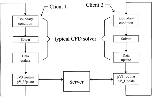
Figure 1.1 Interaction between the server and clients in a typical 2-client setup ... 16

Figure 1.2 pV 3 user interface. ... 17

Figure 2.1 Illustration of a streamline with 5 segments ... ... 20

Figure 2.2 Illustration for particle integration in a 3-client setup... 23

Figure 2.3 Integration of a particle requiring a transfer from client 1 to client 2 and a re-transfer from 2 back to 1 ... ... 25

Figure 2.4 Illustration of a particle requiring 3 transfers ... ... 27

Figure 3.1 Flow pattern at a critical point whose velocity-gradient tensor has 1 real and a pair of complex-conjugate eigenvalues ... 30

Figure 3.2a A hexahedron (or structured-grid cell) divided into 6 tetrahedra ... 31

Figure 3.2b A prism cell divided into 3 tetrahedra ... 32

Figure 3.2c A pyramid cell divided into 2 tetrahedra. ... ... 32

Figure 3.3 A sample result of an artificially-generated test case ... 35

Figure 3.4b flow past a tapered cylinder. Swirl flow centers and streamlines are shown ... 37

Figure 3.4a Flow past a tapered cylinder. Shown are swirl flow centers found by the algorithm.37 Figure 3.5 Flow over a F117 fighter. Swirl flow centers and streamlines are shown. Note: The centers are not mirrored... ... 38

Figure 3.4c B low up of figure 4b ... 38

Figure 3.6a Result of FAST vortex core finder on data set 1 ... 39

Figure 3.6b Result of pV3 swirl flow finder on data set 1... ... 39

Figure 3.6c Result of FAST vortex core finder on data set 2 ... 40

Figure 3.6d Result of pV3 swirl flow finder on data set 2... ... 40

(7)

Figure 3.6e Result of FAST vortex core finder on data set 3. Note that a streamline has also been spawned here to indicate that the twist at the top of the middle curve is actually

outside the vortex. ... ... 4 1 Figure 4.1 Pseudo-mesh cell P (dashed) surrounding node i and a cell neighbor A. The corners

of P are composed of the center of neighboring cells marked by capital letters... 46

Figure 4.2 Face and node numbering for hexahedral cell ... ... 47

Figure 4.3 Stencil for pseudo-Laplacian. Only cell A is shown. ... 50

Figure 4.4b Residence-time contours for flow shown in Fig. 4.4a ... .51

Figure 4.4a Artificially-generated flow with constant velocity in the x direction, vx = 1...51

Figure 4.5a Swirling flow through a converging-diverging duct [11]. A separation bubble is shown as an iso-surface of streamfunction with value 0. Streamlines are also shown...52

Figure 4.5b Contours of residence time for flow through a converging-diverging duct. ... 53

Figure 4.5c Contours of residence time and iso-surface of streamfunction with value 0... 53

Figure 4.5d Iso-surface of residence time of value 27.5... ... 53

Figure 4.6a Mesh at the hub of the stator/rotor (stator: 40 x 15 x 15, rotor: 40 x 15 x 15). Dashed line segments indicate periodic boundaries ... ... 54

Figure 4.6b 3-D illustration of stator/rotor passage. Grey area is the hub ... 55

Figure 4.7 Nodes at the stator/rotor interface. Solid circles indicate actual nodes. Unfilled circles indicate locations corresponding to actual nodes at the opposite interface ... 56

Figure 4.8 Nodes at non-overlapping region can be mapped to location at the opposite interface by using the periodicity assumption ... 56

Figure 4.9a Residence-time contours at the hub. Regions where anomalies occur are indicated by dashed circles .. ... 58

Figure 4.9b Residence time contours at the tip. Regions with anomalies are similar to the ones show n in Fig. 4.9a... 60

Figure 4.10 Residence time iso-surface of value 7.7. For clarity, rotor blade surfaces are not show n... ... ... ... ... 61

Figure 4.11 Residence time iso-surface of value 11.0 ... 61

Figure 4.13a Mach number contours at the hub. Regions with large gradient indicated by dashed circles . ... 62

(8)

Figure 4.12 Region B (of Fig. 4.9a) enlarged to show an unrealistically-large gradient of

residence tim e ... ... 62 Figure 4.13b Mach number contours. Region (at the stator suction surface near the trailing edge) w ith large gradient... ... 63 Figure 4.13c Mach number contours at the tip. Regions with large gradient indicate by dashed

circles ... 63 Figure 4.13d Density contours. Density non-dimensionalized by the inlet stagnation density.

Regions with large gradient indicated by dashed circles ... 64 Figure 4.13e Density contours. A region with large density gradient (at the stator suction surface near the trailing edge). ... 64 Figure 4.13f Density contours. A region with large density gradient (near the trailing edge of the

stator pressure surface) ... 65 Figure A. 1 Pseudo-mesh cell P (dashed) surrounding node i and a cell neighbor A. The corners

of P are composed of the center of neighboring cells marked by capital letters ... 73 Figure A.2 Face and node numbering for hexahedral cell. ... 74

Figure A.3 Contributions of cell A to the first-order (left), and the second-order (right) flux integration . ... 75 Figure B. 1 Flow patterns for selected distributions of eigenvalues of the velocity-gradient

tensor ... ... ... ... 77 Figure B.2a Flow separating at a 3-degree angle from the specified separation plane (dotted line).

Velocity is zero and uniform in the z direction ... ... 80 Figure B.2b Side view of separating flow and the surface found by the separation-flow-finder

algorithm . ... 80 Figure B.2c Separation surface shown in Fig. B.2b. Velocity vector cloud not shown... 81 Figure B.3a Flow moving in opposite direction divided by a separation plane (dotted line).

Velocity in is zero and uniform in the z direction. ... 81 Figure B.3b Side view of opposing flow and the surface found by the separation-flow-finder

algorithm . ... 82 Figure B.3c Separation surface shown in Fig. B.3b. Velocity vector cloud not shown ... 82 Figure B.4a Swirling flow through a converging-diverging duct [11]. A separation bubble is

(9)

Figure B.4b Surfaces found by the separation-flow-finder algorithm. ... 83 Figure B.4c Enlargem ent of Fig. B.4b... ... 84 Figure B.4d Separation surfaces and streamfunction iso-surface overlapped... 84

(10)

List of Tables

(11)

Nomenclature

F, G, H the quantities in the residence-time equation that are x, y, and z differentiated, respectively

Q the non-derivative term in the residence-time equation

Sx, Sy, Sz projected areas on xz, yz, and xy plane of a face of a hexahedral cell U the quantity in the residence-time equation that is time differentiated

V cell volume

X eigenvector

t time

u,v,w velocity

w reduced velocity

x,y,z spatial coordinates

Greek , eigenvalue Ct viscosity p density I residence time Superscripts

n index of discretized time

averaged quantity

Subscripts

i, j, k referring to the Cartesian coordinate directions i a node in a discrete computational domain

(12)

Chapter 1 Introduction

Understanding 3-D transient CFD data is difficult. The additional spatial and time dimensions generate considerably more information than 2-D steady calculations. Furthermore, the increasing complexity of the type of flow being simulated introduces numerous flow features investigators will find of interest, such as vortices, separation bubbles, and shock interactions. All of these directly impact the amount of effort needed to study and interpret such data.

To aid investigators in this effort, various visualization software (as well as

software/hardware) packages have been developed. While most of these systems share many similar features, new and unique concepts are constantly being developed in order to achieve the ultimate goal, a better understanding of the data. For instance, the Virtual Windtunnel [5]

immerses the user within the data by employing a six-degree-of-freedom head-position-sensitive stereo CRT system for viewing. A hand-position-sensitive glove controller is used for

manipulating the visualization tools within the virtual flow field. Systems such as AVS [36] [7] and Khoros [33] [32] uses a visual programming environment in an attempt to ease and expedite the programming process. In the data-flow visual programming environment, the user defines the processing to be done on the data graphically, using icons to represent the processors and links between icons to represent the flow of data. At the other end of the spectrum, pV3 [19] [20] employs a more conventional programming (through subroutine calls) and a straight forward and easy to learn user interface. It is designed for distributed computing and co-processing, allowing for scaleable compute power for large data sets.

To facilitate the investigation of the data, these packages provide many common visualization tools, which can be categorized according to their capabilities [8] [16]: feature identification, scanning, and probing. Feature identification tools, such as a shock detector, enable the users to find particular features of the flow quickly. Scanning tools, such as cutting surfaces and iso-surfaces, provide a way to incrementally view the domain by specifying either a spatial or a scalar

(13)

parameter. Probing tools, such as instantaneous streamlines, streamline probe, and point probe, provide the most localized information, the behavior of the flow or the values of a particular flow

quantity at certain point(s). This categorization also reflects the reduction of dimensionality of the information in the data, from 3-D to 0-D, which is sometimes necessary in understanding the various aspects of the flow.

These tools can be effective because they provide the users information based on the data in a form that can be absorbed more easily. For instance, streamlines show how the vector fields behave, and using it is usually more effective in comprehending the flow field than looking at pages of raw numbers. Iso-surfaces provide information on the scalar fields in the data by generating surfaces where the scalar field has a specified value, which concisely describes a particular distribution within the domain.

Also crucial in the effectiveness in the use of these tools is the speed at which they can be manipulated interactively. In investigating the vast amounts of data produced by the CFD solvers, the users will need to orient and re-orient cutting surfaces around the domain, spawn streamlines, and generate iso-surfaces. An almost instant feedback is required so as not to break the users' train of thought during the investigation. For any particular tool, the feedback time depends mainly on the size of the domain, the capability of the computer, and the number of other tools being requested.

In recent years, unsteady 3-D simulations have become more common, and their size has increased steadily. Along with this growth comes a demand for a visualization software capable of handling huge 3-D unsteady data as well as providing tools for interrogating that data. To meet this goal, a parallel visualization software, called pV3 has been developed at MIT [19] [20]. pV3 is designed for co-processing and also distributed computing. Co-processing allows the investigator to visualize the data as it is being computed by the solver. Distributed computing decomposes the computational domain into 2 or more sub-domains which can be processed across a network of workstation(s) and other types of compute engines. Thus, the processing needed by the visualization-tool algorithms (e.g., finding iso-surfaces, integrating particles and streamlines, etc.) can be done in parallel. With parallel processing, the compute power can be scaled with the size of the problem, thus maintaining the desired interactivity.

(14)

The computation of some of the visualization tools, such as iso-surfaces and cutting planes, are embarrassingly parallel since they are done on a cell-by-cell basis. As such, these

computations are automatically parallelized when the computational domain is decomposed. However, domain decomposition brings up concerns regarding the where and how a particle-path or streamline integration can continue when the integration crosses a sub-domain boundary (also called internal boundary). This is not an issue in a single-domain environment, in which a particle-path or streamline calculation stops when the integration reaches the domain boundary. One of the aims of this thesis is to present a method for managing the information movement needed to continue integrations across these internal boundaries.

Parallel processing also invites opportunities to develop visualization tools that can take advantage of distributed compute power. As noted by Haimes [16], the weakest link in visualization is probably the scarcity of feature identification tools. Thus, the second and third thrust of this work is to present two new feature identification tools, a swirling-flow finder and a residence-time integrator, whose computations are designed to be parallel. A swirling-flow finder

automatically identifies the center of swirling flows and displays the center as a series of disjoint line segments. A residence-time integrator computes the amount of time the fluid has been within the computational domain. These tools provide alternative ways of looking at the data and its

features, and it is hoped that they can present new insights which lead into better understanding of the data and the underlying physics.

1.1 Thesis Outline

Since all the work and development that will be presented here are done within the context of pV3, a brief description of pV3 and its environment will be given in the next section.

Chapter 2 describes how domain decomposition effects the integration of streamlines and particle paths, and the issues and problems encountered in continuing integration across sub-domain boundaries. A solution that takes into consideration issues such as minimizing network traffic and maximizing the use of the parallel environment will then be presented.

(15)

Chapter 3 first presents the motivation for the development of the swirling-flow identification tool. The fundamental theory and its implementation will then be explained. And finally, some result validation will be shown.

The algorithm used in computing residence time is discussed in chapter 4. The development of the governing equations of residence time for various types of flow (inviscid incompressible, inviscid compressible, viscous compressible, and constant density and viscosity) and some sample calculations will also be presented.

Finally, the contributions of this work will be summarized in chapter 5.

1.2 pV3

pV3 is the latest in a series of visualization software developed at MIT. The previous generation software, Visual2 [13] and Visual3 [17] [18], are designed for visualizing two and three dimensional data in a post-processing manner. On the other hand, pV3 is designed for co-processing visualization of unsteady data whereby the user can visualize the results as the model or solver progresses in time. pV3 also allows the solution to be computed in a distributed/parallel environment, such as in a multi-workstation environment or in a parallel machine. In such a setup, the movement of visualization data between the solver machines and the visualization workstation will be taken care of by pV3. The development of pV3 was motivated by the

increase in size of 3-D unsteady calculation and the need for highly interactive tools in visualizing and interrogating the results [19].

In the distributed solver model of pV3, the CFD system/solver decomposes the

computational domain into sub-domains. The computational domain is made up of elements (such as tetrahedra, hexahedra, etc.), and the sub-domain boundaries are formed by the facets of these elements. pV3 accepts any combination of these elements: disjointed cells (tetrahedra, pyramids, prisms, and hexahedra), poly-tetrahedral strips, and structured blocks. In pV3, the programmer can specify where a streamline/particle-path integration should continue (to a cell in a specific domain, through a specific internal boundary in a domain, or to try all

(16)

Figure 1.1 Interaction between the server and clients in a typical 2-client setup.

Each sub-domain is handled by a separate process (called a client in pV3), and each computer in the distributed environment can execute one or more client(s). The user interface and graphic rendering are handled by a process (called the server) run on a graphics workstation. As an illustration, the interaction between the server and the clients in a typical 2-client setup is shown in Fig. 1.1. A call to a pV3 subroutine (named pV_Update) is added to a typical CFD solver to handle the processing needed by pV3, including particle-path and streamline integrations. To keep the processing synchronized, each client does not exit pV_Update until the server transmits

a time-frame-termination message. Only then can the clients continue to the next time step. From the user's point of view, pV3 consists of a collection of windows, which includes a 3D, 2D, and 1D window, as illustrated in Fig. 1.2. Objects such as computational boundaries,

iso-surfaces, streamlines, or cutting planes are shown in the 3D window. The mapping of the cutting plane or contours are shown in the 2D window. The ID window displays one dimensional data generated by various probing functions of the 2D window or from mapping the values traced along a streamline. This arrangement, in conjunction with reduction of dimensionality provided

(17)

3D Window

Key Window -/ -o *, . dwi i ,,

2D Window

Dialbox Window

@'AJAA

i D Window

Text Window . i .

Figure 1.2 pV3 user interface.

by the visualization tools, enable the user to simultaneously consider several aspects of the data, and thus facilitating the comprehension of complex 3-D data.

Interactions with pV3 -for orienting objects in the 2D or 3D window, activating visualization tools, modifying tool parameters, etc. -are done through mouse clicks and keyboard inputs within the various windows. By entering text strings in the pV3 text window, the user can interact with the solver by sending messages which are then interpreted by programmer-supplied routines in the solver. This capability, which is unique among visualization software, enables the user to steer the solution while simultaneously visualizing the results.

(18)

Chapter 2 Integration of Particle Path and Streamline

across Internal Boundaries

2.1 Particle-Path and Streamline Integration

A streamline is a curve in space which is everywhere tangent to the instantaneous velocity field. It is calculated by integrating:

- u() (2.1)

da

where i is the position vector, ii the velocity vector, and a the pseudo-time variable. The integration employs a fourth-order Runge Kutta method with variable pseudo-time stepping. The pseudo-time variable is used only for integrating streamlines and is independent of the actual computation time-step.

A particle path, on the other hand, represents the movement of a massless particle as time

progresses. The calculation amounts to integrating:

d-

=(', t) (2.2)

dt

The integration uses a fourth-order accurate (in time) backward differencing formula. Details about the streamline and particle path integration algorithms can be found in [9] [10].

Both types of integrations start at a user-specified seed point and end when a computational boundary is reached. However, between these points the integration might pass through one or more sub-domain boundaries. When this occurs, information needed in continuing the integration (referred to as a "continue-integration request" or "transfer request") must be sent to other client(s) so that the integration can continue. The information usually comprises of integration state, identification number for the particle/streamline, rendering options, the identification of the

(19)

client sending the request, etc. As stated in section 1.2, the CFD system can specify where an integration should continue when it crosses an internal boundary. However, this specification might be erroneous, or it might not be applicable in certain flow conditions. Thus, for robustness, the system should try its best to continue an integration despite an incorrect instruction. For this reason the client(s) receiving the transfer request has the option to do one of the following:

* accept the transfer: determines that the integration continues in its sub-domain and proceeds with the integration.

* reject the transfer: determines that the integration does not continue in its sub-domain and ignore the request.

* request a re-transfer: determines that the integration does not continue in its sub-domain and requests that the integration be continued in one or more other client(s).

The algorithm for determining whether an integration hits an internal boundary, or whether a client accepts/rejects a transfer, or requests a re-transfer involves checking the spatial location used in the current integration stage against the sub-domain space. The details of this method will not be discussed in this thesis, but can be found in [9]. Here, only the problems encountered in managing transfer requests will be addressed, as well as how the client(s) and the server must interact to ensure that integrations are continued, while keeping the process as efficient as possible. The issues can be stated with the following questions:

* Due to the possibility of re-transfer, how can sending the same request to the same client(s) repeatedly be avoided? This is a question of efficiency as well as avoiding multiple instances of the same object within a sub-domain.

* How can the server know when to safely send the time-frame-termination message? Sending this message when there is a possibility of further integration transfers could prematurely abort the integration of some particles or streamlines. Thus, the server must know when all

transfers are complete for the current time step. Otherwise, the time-frame-termination signal can not be sent and the clients (involving the CFD solver) will remain in a wait state, stalling the entire calculation. In this case, the graphics server will eventually time-out due to

(20)

sub-domain boundary

Figure 2.1 Illustration of a streamline with 5 segments

inactivity, release the clients from this wait state, and quit. This situation is clearly undesirable.

What is the best way to maximize the use of the parallel environment in integrating streamlines and particle paths? These integrations are essentially a serial process. The integration starts at some point at the beginning of the time step and stops at another point at the end of the time step. In between, the process must be done in a certain order. In pV3's parallel

environment, the work of integrating streamlines/particles can be distributed because each client processes only the objects in its sub-domain. However, problems in optimally exploiting the distributed environment can occur due to the need to continue integration across internal boundaries and also the existence of other types of requests (most of which are embarrassingly parallel) that the clients need to handle. It can be foreseen that there could be cases where a mixture of transfer requests and other requests could generate a load imbalance between the clients. The problem can be alleviated (thus, maximizing the use of the parallel environment)

by prioritizing requests in a certain manner. This issue will be illustrated and made clearer

when the solution is discussed in the next section.

When it comes time for rendering, each client sends the server the relevant information about all the particles (i.e., their locations) that end up in its sub-domain at the end of the current time step. A streamline, however, is divided into segments. A new segment begins every time a streamline integration crosses an internal boundary. For example, a streamline with 5 segments is illustrated in Fig. 2.1. To render a streamline, each client sends the server information about the

Client 1 Client 2 Client 3 segment 4 segment 5

seed :

point_ "-

-segment 1 segment 2 segment 3 computation boundary

(21)

segments (e.g., the points forming the segment) within its sub-domain. The server combines the segments, constructs a complete streamline and then renders it.

Although, the underlying construction of a particle and a streamline are completely different, the issues encountered in continuing their integration across an internal boundary are in fact similar. For a particle, the question is where it should end up at the end of the current time step. For a streamline, the question is where its next segment should begin at the end of the current pseudo-time step. This similarity will be exploited in developing a scheme that is usable in both cases. The evolution of this scheme will be described in the next section.

2.2 Solution

First, the following scheme is proposed:

1. It is decided to process transfer request (TR) through the server instead of having the clients communicate directly. Thus, to continue the integration of a particle/streamline, a client sends a TR to the server, which then distributes it to one or more client(s), depending on the

particular internal-boundary specification. This solution provides a simpler and cleaner system overall because all other visualization message traffic is client-server and only one process (the server) needs to manage the transfer requests. Since solver messages are client-client, the risk of interfering with solver messages is also minimized.

2. For each particle/streamline segment that requires transfer across internal boundary, the server keeps a list of clients to which the TR have been sent. The server also assigns a unique

identification number (denoted by TID, for "transfer id") for each of these particles/streamline segments.

3. To prevent sending the same TR to a client, the server can send a TR for a TID to a particular client only if the client is not already in the client list. Thus, to avoid sending a transfer

request back to the originating client (i.e., the client which initially sends the transfer request), the originating client must automatically be logged in the client list.

(22)

4. Transfer requests have higher priorities (at the client and the server) over other types of visualization requests. Thus, if the request queue of a client or the server contains a TR, that request will be handled before other types of requests. In most situations, this procedure will help lessen load imbalances. As an example, consider a 3-client setup where the request queue of client 2 contains R1, R2, and lastly a transfer request TR, while that of client 1 and 3 contains only R1 and R2. R1 and R2 could be requests to calculate iso-surfaces, find swirling flow, generate cut planes, etc. Let's suppose that TR will generate a re-transfer to client 3. Requests R1 and R2 could take much longer to process in client 2 than in client 3, depending on the size of the sub-domains, the type of request, and the flow conditions. If the clients handle the requests according to their order in the queue (i.e., R1 first, R2 second, and so on), client 3 will finish before client 2. Client 3 will have to wait until client 2 handles the transfer request before it can process the re-transfer that will be generated by that request. On the other hand, if TR has higher priority and is processed first by client 2, client 3 will receive the re-transfer sooner. The entire process will take less wall-clock time than without prioritizing.

5. After a client processes a TR -whether accepting, rejecting, or re-transferring the request -it sends a transfer-processed acknowledgment (TPA) back to the server. Since the originating client is automatically logged in the client list, a TPA is also automatically associated with the

originating client.

6. The transfer process for a particular TID is completed when the server receives TPAs from all the clients to which the TID has been transferred. To simplify the algorithm for checking transfer completion it must be ensured that when a client sends a TR and then a TPA (such as in a re-transfer request), the server receives them in the same order. Then, the server will record the re-transfer (if any is allowed) before the TPA. This can be accomplished by setting TPA's priority to be the same as TR's. Now, determining transfer completion can be done at any moment by identifying those TIDs whose client list has a complete set of TPAs. When all TIDs have a matching set of clients and TPAs, the server knows that no more transfers will be requested during the current time step.

(23)

Client 1 Client 2 Client 3

TID 1 TID 3 * O

*---, O -- O

TID 2

WI . " O

a- b sub-domain boundary specification. Indicates that integration should try to continue in client "a" if integration approaches from the left, in

client "b" if from the riaht. "*" indicates all clients. * particle location prior to integration

O particle location after integration

Figure 2.2 Illustration for particle integration in a 3-client setup.

To illustrate this scheme, a 3-client example is shown in Fig. 2.2. In this example 3 particles require transfers in the current time-step and 1 particle does not. Note that no transfer will be requested for the fourth particle (the one in client 3) because it stays within client number 3. Due to the similarity in continuing particle and streamline integration, only examples for particles will be shown. In a step-by-step manner, the scheme works as follows (at each step, the particle transfer log for each TID is summarized in the corresponding table):

1. The server receives two transfer requests from client 1 and one from client 2, and assigns them TID 1, 2, and 3 as shown in Fig. 2.2. In the tables below, "cl." stands for client, and a

"/" under a client number indicates that a TR has been sent to that client (or the client is the

originating client), and a "V"' under TPA means that the server has received a TPA from the corresponding client. Complying with the internal-boundary specification, the server transfers TID 1 and 2 to client 2, and attempts to transfer TID 3 to client 1, 2, and 3. However, since TID 3 already has client 2 in its transfer list, TID 3 will not be transferred there again. Note that a TPA is automatically assigned to the originating client.

computation boundary sub-domain boundary

(24)

Transfer history of TID 1

cl. TPA c1.2 TPA Ic. 3 TPA

Transfer history of TID 1

cl. I TPA cI. 2 TPA cl 3 TPA

cl. 1 TPA cl. 2 TPA cl. 3 TPA

, s

Transfer history of TID 2 c. 1 TPA I c. 2 TPA cl. 3 TPA

cl. 1 TPA c.

2 TPA cl. 3 TPA

cl. 1 TPA cl.2 TPA cl. 3 TPA

I/ I I/

cl. I TPA c1.2 TPA cl.3 TPA

cl. I TPA cl. 2 TPA cl. 3 TPA

S S/

2. Client 1 will reject TID 3 and send a TPA. Client 2 will accept TID 1 and send a TPA. Client 2 will also request that TID 2 be re-transferred to all other clients, and then send a TPA for TID 2. However, since client 1 and 2 are already in the client list of TID 2, TID 2 will only be transferred to client 3. Client 3 will accept TID 3 and send a TPA. At the end of this step the transfer process for TID 1 and 3 is complete because each client in their list is paired with a

corresponding TPA.

55/sJI

Transfer his ory of TD 2

V V V 5 I/ I/

cl. 1 TPA c.2 TPA cl. 3 TPA / V/ I/ I/"

3. Client 3 accepts TID 2 and sends a TPA. At this point (and only at this point), all TID have a

complete list of TPAs (i.e., each client in the list is paired with a TPA). Thus, all transfers are complete for this time step.

cl. 1 TPA c. 2 TPA cl. 3 TPA

cl. 1 TPA cl. 2 TPA cl. 3 TPA

55/555 J

55/sJ

(25)

A ,, i sub-domain boundary / * / \

Client 1

Client 2

Figure 2.3 Integration of a particle requiring a transfer from client 1 to client 2 and a re-transfer from 2 back to 1.

Now consider the situation illustrated in Fig. 2.3. Initially, client 1 transfers the particle to client 2, then client 2 requests a re-transfer back to client 1. However, since the particle originally comes from client 1, the above scheme will not allow this, and the integration stops. To take care of cases such as this, the above scheme is modified to allow a particle (or streamline segment) to be transferred to the same client twice. Since multiple transfers to the same client are now allowed, there is no need to automatically include the originating client in the client list. For the situation in Fig. 2.3, the process goes as follows:

1. The server receives a transfer request from client 1, and transfer the integration to client 2. In the table below, there are now 2 columns under client and TPA to reflect that the particle can be transferred to the same client twice.

Client 1 TPA Client 2 TPA

V.

(26)

/ I,/ I €"

3. Client 1 accepts the transfer and sends a TPA. At this point every check mark in the client column is paired with a check mark in the TPA column, indicating the transfer process for the current time step is complete.

V V

This solution, however, is not without trade-offs and limitation. In cases where re-transfers to the same client are not needed (such as in the first example above), unnecessary multiple transfers to a client might be made. In some situations, a client might accept a transfer twice, creating 2 instances of the same particle (or streamline segment). To prevent this, every time a client receives a transfer request it checks whether it has previously accepted the object. If it has, the request is ignored. The checking is done by comparing the global identification number, which is unique through the duration of the visualization session, or the TID, which is unique during each time step.

This solution is also not a general one. Consider the situation shown in Fig. 2.4, in which the particle needs 3 transfers to client 2. This will not be possible without increasing the maximum number of transfers to 3, which will further reduce the efficiency of the scheme. It can be seen that however large this number is set to, the solution will never be general. Thus, as a trade-off between efficiency and more generality the number of transfers have been limited to 2. This limit will cover most cases without significantly compromising efficiency. Should a particle-path integration require more than two visits to the same client, the integration will abort and the particle will be "lost". If it is a streamline integration, only part of the streamline will be rendered (from the seed point to the last point before the unsuccessful integration transfer). Fortunately, this limit is not too severe in most instances. The streamline integration algorithm uses a pseudo-time step limiter, which is based on the cell size as well as local vector field data. This limiter insures that the next requested point in the integration is no more than the cell's size from the

(27)

Client 1 0 '.. . 00 2 ... ... ...... Client 2 sub-domain boundary

Figure 2.4 Illustration of a particle requiring 3 transfers.

current position. If the size of the neighboring elements do not change drastically, the problems posed by this scheme will be minimal. In a flow computed using an explicit scheme, the time step governed by the CFL stability requirement of the flow solver will generally limit the movement of a particle to no further than the adjacent cells.

(28)

Chapter 3 Swirl Flow Finder

This work is motivated by the need to easily locate vortices in large 3-D transient problems. A tool that will automatically identify such structures is definitely needed to avoid the time-consuming and tedious task of manually examining the data. However, the question of what defines a vortex raises considerable confusion. As a result, various definitions of a vortex and methods for identifying vortices have been proposed by investigators.

Moin and Kim [28] [27] propose the identification of vorticity using vorticity lines, which are integral curves of vorticity. However, this method is found to be very sensitive to the starting point of the integration. Moin and Kim [28] indicate that a badly chosen initial point will likely result in a vortex line which wanders over the entire flow field, making it difficult to identify any coherent structures.

Chong, Perry, and Cantwell [6] propose a definition based on the eigenvalues of the velocity-gradient tensor. A vortex core is defined as a region with complex eigenvalues, which means the local streamline has a helical pattern when viewed in a reference frame moving with the local flow.

By incorporating some of the work of Yates and Chapman [39] and Perry and Hornung [31], Globus, Levit, and Lasinski [14] identify vortices by first finding a velocity critical point where the velocity-gradient tensor has complex eigenvalues. The vortex core is found by integrating,

starting from the critical point, in the direction of the eigenvector corresponding to the only real eigenvalue.

Banks and Singer [3] [4] propose an algorithm which finds the vortex core by using a predictor-corrector scheme. The vorticity vector fields is used as the predictor and the pressure gradient as the corrector. This scheme is designed to self-correct toward the vortex core.

Jeong and Hussain [25] propose a definition of a vortex in incompressible flow in terms of the eigenvalues of the tensor S2₊ 2_{, where S and Q are the symmetric and antisymmetric parts}

(29)

of the velocity gradient tensor. A vortex core is defined as a connected region with two negative values of S2 + j22

These are merely a sample of the works that have been done on this subject. For a more thorough survey, the reader can refer to [4] and [25], both of which discuss the inadequacies and limitations of the various schemes.

Considering the confusion that still exists on what constitutes a vortex and the limitations of existing schemes, this author believes that there is a need for a tool that can help investigators locate vortices, and yet has a familiar and intuitive interpretation. To achieve this goal, the condition that what the tool finds must be vortices will be relaxed. However, the scheme must be practical, in terms of computational speed and usability.

This work proposes that a tool which identifies the center of swirling flows satisfies the above need and criteria. Investigators have been using swirling flow as one of the means to locate vortices in 3-D discretized vector fields. Swirling flows in a 3-D field are usually identified by studying vector fields which are mapped onto planar cuts or by seeding streamlines. These procedures can be very laborious, especially for large and complex flows. The scheme presented here allows automatic identification of the center of swirling flows in 3-D vector fields.

The algorithm for implementing this tool is based on critical-point theory. As will be

described below, the scheme works on a cell by cell basis, lending itself to parallel processing, and is flexible enough to work with the various types of grids supported by pV3. With this method, the need for curve integration (which is needed for visualization tools such as streamlines and particle paths) has been avoided. Curve integration is a serial operation and can not readily take advantage of pV3's distributed computing capabilities. And, as described in chapter 2,

integrations across a distributed environment involve passing information between machines and other additional complexities which further reduce efficiency.

In the next sections, the theoretical background of this algorithm and its implementation will be described. The results of the scheme on exact artificially-generated data as well as CFD data will be shown. Results will also be compared (using artificially-generated data) against those from a tool developed by Globus, Levit,and Lasinski [14].

(30)

Figure 3.1 Flow pattern at a critical point whose velocity-gradient tensor has 1 real and a pair of complex-conjugate

eigenvalues.

3.1 Theory

Critical points are defined as points where the streamline slope is indeterminate and the velocity is zero relative to an appropriate observer [6]. According to critical point theory, the eigenvalues and eigenvectors of the velocity-gradient tensor, Dui/xj (this matrix will be called A), evaluated at a critical point defines the flow pattern about that point. Specifically, if A has one real and a pair of complex-conjugate eigenvalues the flow forms a spiral-saddle pattern, as

illustrated in Fig. 3.1. The eigenvector corresponding to the real eigenvalue points in the direction about which the flow spirals, and consequently, the plane normal to this eigenvector defines the plane on which the flow spirals. For a complete description of all other possible trajectories the reader can refer to [6] or [1].

The pattern in Fig. 3.1 is intuitively recognized as swirling flow, and, therefore the above method can be used to find the center of swirling flows located at critical points. However, there are obviously swirling flows whose center is not at a critical point. Fortunately, a similar method can be applied in these cases.

(31)

At a non-critical point with the necessary eigenvalue combination (i.e., one real and a pair of complex conjugates) the velocity in the direction of the eigenvector corresponding to the real eigenvalue is subtracted. The invariance of the eigenvectors' directions with respect to a Galilean transformation ensures that the resulting flow will have the same principal directions. The

resulting velocity vector will be called the reduced velocity. If the reduced velocity is zero, then the point must be at the center of the swirling flow. A similar statement was also made by Vollmers, Kreplin, and Meier [38].

Therefore, to find a point at the center of a local swirling flow, the algorithm searches for a point whose velocity-gradient tensor has one real and a pair of complex-conjugate eigenvalues and whose reduced velocity is zero.

3.2 Implementation

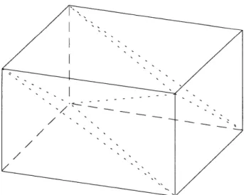
pV3 accepts structured and/or unstructured grids (containing any combination of tetrahedra, polytetrahedra strips, hexahedra, pyramids, and prism cells). In the interest of efficiency, only tetrahedral cells are used, with all other cell types reduced to 2 or more tetrahedra. Fig. 3.2 shows how various types of cells are decomposed into tetrahedral cells.

Figure 3.2a A hexahedron (or structured-grid cell) divided into 6 tetrahedra.

(32)

Figure 3.2b A prism cell divided into 3 Figure 3.2c A pyramid cell divided into 2

tetrahedra. tetrahedra.

This approach allows the use a simple linear interpolation for the velocity, avoiding the more complex, and inherently more costly, interpolation required by other types of cells (such as bilinear interpolation for hexahedra). A tetrahedron has 4 node points, sufficient to solve for the four coefficients of a 3-D linear interpolant. More importantly, linear velocity interpolation produces a constant velocity-gradient tensor within the entire tetrahedral cell. Consequently, the straight forward algorithm described below can be employed, which otherwise would not have been possible.

The algorithm proceeds one tetrahedral cell at a time, and can be summarized as follows (it is assumed that a velocity vector is available at each node):

1. Linearly interpolate the velocity within the cell.

2. Compute the velocity-gradient tensor A. Since a linear interpolation of the velocity within the cell can be written as

ui = Ci + U A + Ay + Az (3.1)

then A can be constructed from the coefficients of the linear interpolation function of the velocity vector.

(33)

3. Find the eigenvalues of A. Processing continues only if A has one real (kR) and a pair of complex-conjugate eigenvalues (kC).

4. At each node of the tetrahedron, subtract the velocity component in the direction of the eigenvector corresponding to XR. This is equivalent to projecting the velocity onto the plane normal to the eigenvector belonging to XR , and can be expressed as

i = i - (i -i)i (3.2)

where i is the normalized eigenvector corresponding to XR, and w is the reduced velocity.

5. Linearly interpolate each component of the reduced velocity to obtain

wi = ai + bix + cy+ diz (3.3)

i=1, 2, 3

6. To find the center, set wi in Eqn. (3.3) to zero. Since the reduced velocity lies in a plane, it has only 2 degrees of freedom. Thus, only 2 of the 3 equations in Eqn. (3.3) are independent.

Any 2 can be chosen as long as their coefficients are not all zero.

0= ai + bix + cy+ diz (3.4)

i=1, 2

which are the equations of 2 planes, whose solution (the intersection of 2 planes) is a line.

7. If this line intersects the cell at more than 1 point, then the cell contains a center of a local

swirling flow. The center is defined by the line segment formed by the 2 intersection points. Since the 2 intersection points lie on the line found in step 6, the reduced velocity at those points must be zero. This suggests a different (but equivalent) and more efficient way to finding the center. This approach renders steps 5, 6, and 7 unnecessary and replaces them with a new

step 5:

5. For each of the tetrahedron's face, determine if there is exactly 1 point on the face where the

reduced velocity is zero. If at the end there are exactly 2 distinct points, then the cell contains a center, which is defined by those 2 points.

(34)

Both approaches have been tried with identical results. Therefore, the second approach is implemented.

3.3 Testing

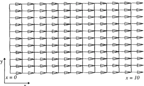
The algorithm is first tested on artificially-generated vector fields where the location of the center of the swirling flow is known exactly. The field is defined by

(5)

u= y-y c ,v=x-xc w=f(z)

Note that this vector field has circular streamlines (in the x-y plane) around a central axis whose location is defined by x, and y,. The magnitude of the vector is equal to the distance from the central axis. The field is discretized using an 11 x 11 x 11 node structured grid. The results for various values of xc, Yc, and functional forms of vz (including constant, linear, and exponential) are

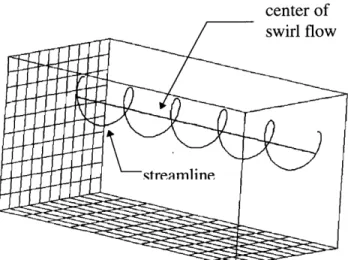
studied and determined to be correct. A sample result (with xc = 2.2 Ax, Yc = 1.5 Ay, and vz = 1) is shown in Fig. 3.3. A streamline is also shown in this figure to provide a sense of the swirling vector field.

Table 3.1 Size of Test Cases for Swirl-Flow Finder Algorithm

Case Number Number Number of Calculation of Nodes of Cells Tetrahedral Time (sec.)**

Cells*

Cylinder 131072 123039 738234 34

F-117 48518 240122 240122 16

* After decomposition (if needed) of original cells. ** On SGI Indigo2 with MIPS R4400 150 Mhz CPU.

(35)

center of swirl flow

Figure 3.3 A sample result of an artificially-generated test case.

Further tests are done using data from 3-D calculations of flow past a tapered cylinder [26] and of flow over an F- 117 fighter at an angle of attack [37]. The tapered-cylinder calculation employs structured grid, while the F-117 case uses unstructured grid composed of tetrahedra. The size of these data sets and the time needed to find the swirl flow centers are summarized in Table 3.1.

The results are shown in Figs. 3.4 and 3.5. To indicate the existence swirling flow, streamlines have been spawned near the centers found by the algorithm. These results indicate that the large coherent structures found by the algorithm do indeed correspond to centers of swirling flow. However, the algorithm does not find all the swirling flow in the tapered cylinder data. Missing are a few swirling flow structures further downstream of the cylinder, which are found by studying the vector field more closely. It is believed that the size of the grid cells might be a factor. The cells are larger away from the cylinder, reducing the accuracy in the calculation of the velocity-gradient tensor (and consequently the reduced velocity). Another possible cause is the algorithm's sensitivity to the strength of the swirl flow. As shown in Figs. 3.4b and 3.4c, the structures are very coherent for strong swirls (i.e., the swirl velocity is larger than or comparable to the normal velocity). However, the structures start to break up as the swirl weakens, and

(36)

further downstream, where the swirl flows are very weak, the algorithm finds no coherent structures.

In the case of the F-117 data, the structures are less coherent than in the tapered cylinder. The tetrahedral grid used in this data is very irregularly sized, and is rather coarse. Comparison between the streamlines in Figs. 3.4c and 3.5 also shows that the swirl in the F117 data is noticeably weaker. Both of these factors might contribute to the incoherence in the structures.

Comparisons have also been done between the results of this algorithm with that of FAST's vortex-core finder [14] [2]. FAST's finder defines a vortex core by integrating from a critical point in the direction of the eigenvector corresponding to the only real eigenvalue of the velocity-gradient tensor. For this comparison, 3 artificially-generated data sets are used, each bounded by a cube containing 3 randomly-placed vortices. The data generator is developed by D. Asimov at NASA Ames Research Center.

The comparisons are shown in Figs. 3.6a to 3.6f. Despite the lack of any 3-dimensional cues, the curves in these figures do exist in 3-D space, and each pair of figures are taken from the same view point. A high degree of similarities are found in each case except for the middle curves in each data set, where FAST produces curves that are either longer and/or has different orientation.

Closer inspection of the data shows that pV3's results are the correct ones, while FAST's curve integrations veer away from the core due to the difficulty in integrating near critical points.

(37)

FLOW

Tapered cylinder

Figure 3.4a Flow past a tapered cylinder. Shown are swirl flow centers found by the algorithm.

Figure 3.4b flow past a tapered cylinder. Swirl flow centers and

(38)

Figure 3.4c Blow up of figure 4b.

A;':9 Cr

Figure 3.5 Flow over a Fl 17 fighter. Swirl flow centers and streamlines are shown. Note: The centers are not mirrored.

(39)

Integration veers away

Figure 3.6a Result of FAST vortex core finder on data set 1.

N _.A

Figure 3.6b Result of pV3 swirl flow finder on data set 1.

(40)

Integration veers away

Figure 3.6c Result of FAST vortex core finder on data set 2.

ii

Figure 3.6d Result of pV3 swirl flow finder on data set 2.

(41)

Figure 3.6e Result of FAST vortex core finder on data set 3. Note that a streamline has also been spawned here to indicate that the twist at the top of the middle curve is

actually outside the vortex.

Figure 3.6f Result of pV3 swirl flow finder on data set 3.

(42)

Chapter 4 Residence Time

Flow separation represents interesting, and sometimes important, features in many types of flow calculations. In turbomachinery, separated flows are associated with extremely hot regions where high-speed hot flow exiting the combustor has been stagnated. These hot spots are very undesirable since the allowable operating stress of the turbine blades are closely related to temperature. In flow over a wing, the adverse pressure gradient on the wing upper surface can lead to separated flow. The major consequences of this phenomenon are a drastic loss of lift (or stalling) and a significant increase in pressure drag.

This interest in separated flow motivates the development of a tool which can automatically locate these regions. Ideally, the tool can work directly on the vector fields at each time slice of an unsteady data, without requiring other types of data or information from other time levels. An attempt was made to develop an algorithm, based on critical point theory, which works solely on the vector fields. However, this scheme was found to be unreliable in detecting separated flows. For documentation, the algorithm is described in Appendix A.

Helman and Hesselink [22] [23] have developed a visualization scheme for generating separation surfaces using only the vector field. The scheme starts by finding the critical points on the surface of the object. Streamlines are integrated along the principal directions of certain classes of critical points and then linked to the critical points to produce a 2-D skeleton of the flow topology near the object. Streamlines are integrated out to the external flow starting from points along certain curves in the skeleton. These streamlines are then tessellated to generate the separation surfaces. With this approach, difficulties might be encountered in integrating

streamlines from critical points, and also in finding separated regions that are not attached to an object. It is also unclear how a recirculation region should be defined in unsteady flows since a region that appears to be recirculating at a time slice might actually be moving with the flow as time progresses.

(43)

Discussions and communications with Haimes [15] and Giles [12] lead to the development of a scheme based on residence time. Essentially, this tool computes the amount of time the fluid has been in (or in residence within) the domain by integrating the residence-time governing equation over time. Time zero is defined as the time when the tool is turned on by the user. Thus, this tool provides information viewed in a frame of reference moving with the fluid, in contrast to streamlines and particle paths which present information viewed from a fixed reference frame.

Most of the fluid within a separation region stays within that region for a considerable amount of time. Thus, a common feature of separation region is that the residence time of the fluid within it is considerably larger than that of the surrounding fluid. The iso-surface tool can then be used to distinguish this region. Therefore, residence time can potentially be used to locate separation regions.

The equations used for computing residence time will be discussed in the first section of this chapter. Section 2 describes how the equations are solved in discretized flow fields. Section 3 and 4 discuss the boundary conditions and the numerical smoothing, respectively. Some sample calculations are shown and discussed in section 5.

4.1 Residence time equation

The residence time of a fluid particle is defined by

Dr

-1 (4.1)

Dt

where I denotes residence time. And since + ii V, then Eqn. (4. 1) becomes

Dt t

+ i- VT =1 (4.2)

at

where i is the velocity vector.

Since the time when the residence time calculation starts is defined as time zero, then initial the condition is

(44)

T (x,y,z) = 0 (4.3) At inflow boundaries, new fluid is entering. By definition, this fluid has zero residence time. Therefore, the boundary condition is

c (x,y,z) = 0 at inflow (4.4)

To obtain the conservative form of Eqn. (4.2) for incompressible flow, Eqn (4.2) can be rewritten as

+ui-VI +' V - =1+, V-ui

at

a

+Vt +-r Vi= 1+ V -ii

at

And since V -ii = 0 for incompressible flow, then

a-

+V- t = 1 (4.5)

at

The conservative form for compressible flow can be obtained by rewriting Eqn. (4.2) as

p- +i- p Vt = p

at

where p denotes density. And since the conservation of mass equation for compressible flow is

ap

a +V- pu=0

at

then

P-- + u. p

_at

_p

+

_It

_ta+

+V-

Pii

P

a _{+ V -(pr ii) = p} (4.6) at

The effect of viscosity on t is similar to its affect on velocity because the same mechanism is at work in both instances. Therefore, the viscous term for Eqn. (4.6) is analogous to the viscous term in the conservation of momentum equation of the Navier Stokes equations. Thus, the residence time equation for a viscous compressible flow is

(45)

S+V- (p' ii)= p+V- _RV'E

or V'T)= p p+V-(p'u- (4.7)

at

where g is the absolute viscosity, which accounts for both laminar and turbulent viscosity. For a flow with constant viscosity and density, Eqn. (4.7) reduces to

-+ V -' ii= 1+ EV2"

t _P

+V. i--u- VT) =1 (4.8)

at _p

where - is constant.

All the conservative forms of the residence-time equation (i.e. Eqns. (4.5), (4.6), (4.7), and (4.8)) can be expressed as

BU aF BG aH

+ + +

Q

(4.9)

at

ax

dy Ez

where, for incompressible inviscid flow

U= , F=' u, G='r v, H=' w, Q=1,

for compressible inviscid flow

U= pt, F= pr u, G= pr v, H= pr w, Q= p,

for compressible viscous flow

U= p, F= pt u- , G= pT v- g , H= pt w- - ,g Q= p

and for a flow with constant viscosity and density

U=', F--- u- , G--- v- H--- w- Q=

p ax p ay pQ z

Note that Eqn. (4.9) has a form similar to the conservative formulation or the Euler equations. This similarity enables the use of an Euler solver developed in another work. The

algorithm, which will be discussed in the next section, operates on a cell-by-cell manner, and, therefore, can readily take advantage of pV3's parallel capability.

(46)

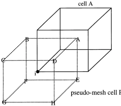
cell A

Figure 4.1 Pseudo-mesh cell P (dashed) surrounding node i and a cell neighbor A. The corners of P are composed of the center

of neighboring cells marked by capital letters.

4.2 Lax-Wendroff algorithm

An explicit time-marching algorithm of Lax-Wendroff type is used to solve Eqn. (4.9). This scheme is identical to that used by Saxer [34] to solve the Euler equations for a stator/rotor flow. The basic integration scheme is similar to the one introduced by Ni [29], recasted by Hall [21], and then extended by Ni and Bogoian [30] to 3-D. Saxer [34] then adapted the formulation to handle unstructured grids, particularly unstructured hexahedral cells.

In solving the residence time equation, it is assumed that the flow variables u, v, w, p, and t are known at all the nodes. The algorithm then computes the flux across each cell face by

averaging the fluxes F, G, and H at the corner nodes. The flux residual is computed by adding the fluxes through the six faces, and then adding the source term for the cell. This residual is then distributed to the eight corner nodes according to the Lax-Wendroff algorithm to evaluate the residence time change at those nodes. The details of the construction of the algorithm are

Distributed visualization and feature identification for 3-D steady and transient flow fields

Distributed

Visualization

and Feature Identification for 3-D

Steady and Transient Flow Fields

FEB 211996

.ari

Distributed Visualization and Feature

Identification

for 3-D

Steady and Transient Flow Fields

Abstract

Acknowledgments

Table of Contents

List of Figures

List of Tables

Nomenclature

Chapter 1

Introduction

1.2 pV3

@'AJAA

Chapter 2

Integration of Particle Path and Streamline

across Internal Boundaries

2.1 Particle-Path and Streamline Integration

cl. I TPA cI. 2 TPA cl 3 TPA

cl. 1 TPA c.

2 TPA cl. 3 TPA

55/sJI

55/sJ

Chapter 3

Swirl Flow Finder

3.1 Theory

3.2 Implementation

3.3 Testing

ii

Chapter 4

Residence Time

4.1 Residence time equation

a

a-

ap

at

P-- + u. p

at

_p

+

It

ta+

+V-

Pii

P

Q

ax

4.2 Lax-Wendroff algorithm

_at

_It

_ta+