HAL Id: insu-02096832
https://hal-insu.archives-ouvertes.fr/insu-02096832
Submitted on 4 Mar 2021
HAL is a multi-disciplinary open access
archive for the deposit and dissemination of
sci-entific research documents, whether they are
pub-lished or not. The documents may come from
teaching and research institutions in France or
abroad, or from public or private research centers.
L’archive ouverte pluridisciplinaire HAL, est
destinée au dépôt et à la diffusion de documents
scientifiques de niveau recherche, publiés ou non,
émanant des établissements d’enseignement et de
recherche français ou étrangers, des laboratoires
publics ou privés.
Global distribution of the solar wind flux and velocity
from SOHO/SWAN during SC-23 and SC-24
Dimitra Koutroumpa, Eric Quémerais, Stéphane Ferron, Walter Schmidt
To cite this version:
Dimitra Koutroumpa, Eric Quémerais, Stéphane Ferron, Walter Schmidt. Global distribution of the
solar wind flux and velocity from SOHO/SWAN during SC-23 and SC-24. Geophysical Research
Letters, American Geophysical Union, 2019, 46 (8), pp.4114-4121. �10.1029/2019GL082402�.
�insu-02096832�
D. Koutroumpa1 , E. Quémerais1 , S. Ferron2, and W. Schmidt3
1LATMOS/IPSL, CNRS, UVSQ Université Paris-Saclay, Sorbonne Universités, Guynacourt, France,2ACRI-ST,
Sophia-Antipolis, France,3Finnish Meteorological Institute, Helsinki, Finland
Abstract
We analyze SOHO (SOlar Heliospheric Observatory)/SWAN (Solar Wind ANisotropy) hydrogen Lyman-𝛼 data collected between 1996 and 2018 to derive the solar wind latitudinal distribution over time. Full-sky interplanetary Lyman-𝛼 maps are inverted to derive the total hydrogen ionization rate latitude profiles, normalized to proton charge-exchange and photoionization. Using Interplanetary Scintillation velocities to calculate the velocity-dependent charge-exchange cross-sections, we produce the solar wind flux latitudinal profiles. Finally, we compute solar wind velocity latitude profiles, based on the dynamic pressure and energy flux conservation (calculated from OMNI data) over latitude. SWAN reproduces the Interplanetary Scintillation velocity profiles up to at least ±60◦, and also agrees with Ulysses in situ measurements for solar minimum periods in 1996–1997 and 2007. During solar maximum, discrepancies are more frequent because in situ data reflect local solar wind conditions, while SWAN data reflect global conditions in the heliosphere.1. Introduction
Since the first systematic observations with the Helios satellites (e.g., Rosenbauer et al., 1977; Schwenn et al., 1981), the solar wind (thereafter noted SW) has been surveyed almost uninterrupted for more than five decades thanks to the large fleet of space missions. The various data taken near the ecliptic (along the Earth-L1 Lagrangian point line) have been intercalibrated into the OMNIWeb/OMNI-2 data set (King & Papitashvili, 2005). Outside the ecliptic, the Ulysses mission has explored the SW properties in a quasi-polar orbit around the Sun for almost 20 years (1990–2009). McComas et al. (2013) have extensively discussed the complete Ulysses data set and the evolution of slow/fast SW properties and the differences in their spatial distributions in the declining phase of Solar Cycle (SC) 22 (1986–1996) and the complete SC-23 (1996–2008). Despite the different properties and latitudinal distribution of the slow and fast SW streams, there are certain physical quantities that are considered to be invariant at all latitudes, that is, independent of SW type. Using plasma data from IMP-8, Ulysses, and Voyager 2 data, Richardson and Wang (1999) have shown that the SW dynamic pressure varies over the solar cycle in the same global way at all latitudes and distances. More recently, Katushkina et al. (2019) also showed that the close correlation of the SW latitudinal pattern found in SOHO (SOlar Heliospheric Observatory)/SWAN (Solar Wind ANisotropy) data and the ENLIL simulations is also most probably due to the fact that the ENLIL simulations assume the conservation of dynamic pressure. Several other studies (e.g., Le Chat et al., 2012; Marsch & Richter, 1984) using HELIOS, Wind, and Ulysses data have demonstrated that the SW energy flux is independent of speed and latitude within 10% and varies weakly over the solar cycle.
The SW latitude distribution has a paramount influence on the interplanetary Lyman-𝛼 glow pattern because interplanetary neutral H atoms are ionized primarily by charge-exchange with SW protons (e.g., Joselyn & Holzer, 1975; Lallement et al., 1985). The concept of the SWAN instrument (Bertaux et al., 1995) on board SOHO was based on this idea. In this paper, we analyze 22 years of SWAN full-sky interplanetary Lyman-𝛼 maps recorded between 1996 and 2018 to derive the global latitudinal SW distribution. In section 2 we describe the SWAN maps, data analysis, and discuss the instrument's performance over time. In section 3 we produce latitudinal distributions of the SW flux and velocities over time, discussing the solar cycle pat-tern evolution and the conservation of SW dynamic pressure and energy flux. In section 4 we compare the results with velocity distributions from the interplanetary scintillation (IPS) data analysis and Ulysses in situ measurements. Finally, we offer some conclusions and perspectives in section 5.
Key Points:
• The SOHO/SWAN instrument is one of the few to derive the global solar wind distribution outside the ecliptic • The data analysis produces latitude
distributions for the solar wind particle flux and velocity as a function of time
• Comparison with IPS and Ulysses velocity data confirms the conservation of dynamic pressure and energy flux in the solar wind
Correspondence to:
D. Koutroumpa,
dimitra.koutroumpa@latmos.ipsl.fr
Citation:
Koutroumpa, D., Quemerais, E., Ferron, S., & Schmidt, W. (2019). Global distribution of the solar wind flux and velocity from SOHO/SWAN during SC-23 and SC-24. Geophysical
Research Letters, 46, 4114–4121. https://doi.org/10.1029/2019GL082402
Received 8 FEB 2019 Accepted 6 APR 2019
Accepted article online 10 APR 2019 Published online 23 APR 2019
©2019. American Geophysical Union. All Rights Reserved.
Geophysical Research Letters
10.1029/2019GL082402
2. SWAN Data: Full-Sky Interplanetary Lyman-
𝜶 Maps and Total H
Ionization Rates
The SOHO/SWAN instrument has been recording full-sky diffuse Lyman-𝛼 emission maps almost uninter-rupted since 1996, except for a period in 1998 when communications with SOHO were lost. Maps have been produced at 1◦×1◦resolution, every 2 days until 2007, and once a day after that. The instrument opera-tions and data processing to retrieve the full-sky Lyman-𝛼 maps are extensively described in (Quémerais et al., 1999, 2006). Except for contamination by bright early-type stars (removed with a mask during the data processing) and occasional comets, the signal is due to the solar Lyman-𝛼 line being backscattered by inter-stellar H atoms permanently flowing through the heliosphere. The H atom distribution is deeply affected by SW mainly through charge-exchange with solar protons which allows to infer SW flux as a function of time and heliolatitude. EUV photons and electron impact also ionize the neutral gas in a lesser extent which we discuss in section 2.1.
The inversion algorithm used to derive the ionization rate from the SWAN maps is described in Quémerais et al. (2006). A forward model with latitude-dependent ionization rates is adjusted to a selection of points in the SWAN maps. The points are spaced on a 5◦×5◦grid to reduce computation times, while points falling within data gaps (due to the star-mask for example) are ignored. The intensity model is computed on a 3-D grid where the space around the Sun is divided in 19 heliographic 10◦-latitude bins. Each bin is characterized by a reference ionization rate𝛽totat 1 AU (the ionization varies everywhere as r−2). Every representative H atom is followed along its trajectory through the heliosphere, and the ionization rate it suffers at a given location is computed according to its heliographic latitude. The local density and velocity distribution is obtained by integrating all possible trajectories. A least-squares adjustment of the reference ionization at 1 AU in each latitude bin is performed for the data selected in each map, converging in average after three iterations. The final result for each latitude bin is representative of a global average ionization rate over large scales in the heliosphere, in opposition to in situ measurements that reflect local conditions in the SW. In the current version of the inversion scheme, the ionization rate at high heliographic latitude is not well constrained. This is due to the fact that the polar regions have a small relative contribution to the total intensities integrated over long lines of sight and are defined by fewer independent data points than other regions. In general, the results of the inversion show larger uncertainties for the polar regions. A total of 4,606 maps were used in the fitting method. For all latitude bins we filter results following two common criteria: (i) when the fit's𝜒2was unsatisfactory (over 3𝜎 of the average 𝜒2); (ii) when data samples
being fitted included less than 780 points (3𝜎 less than the average data sample). Additionally, for individual latitude bins we excluded ionization rates outside the interval𝛽tot= [1 − 10] 10−7s−1. These filters exclude around 150 map fits at low latitude bins and up to ±60◦and between 250 and 590 map fits for the six polar bins (higher than ±70◦), which represents less than 13% of the total map sample for a latitude bin, in the worst case scenario. This confirms that the SWAN fitting method is less reliable at higher latitudes compared with midlatitude to low latitude.
2.1. Normalized Total Ionization Rates
The SWAN absolute calibration has been monitored over the years by interplanetary background measure-ments with the Hubble Space Telescope (HST, e.g., Clarke et al., 1998; Quémerais et al., 2006). In 2008, an International Space Science Institute Working Group compared various UV data sets (e.g., SOHO/SWAN, HST/STIS, Voyager/UVS, New Horizons/Alice, Mars-Ex/SPICAM, Venus-Ex, Cassini-UVIS), resulting in a more accurate definition of the SWAN absolute calibration (Quémerais et al., 2013). A more recent compar-ison to Venus-Express/SPICAV data has shown that SWAN presents a ∼20% sensitivity loss between 2008 and 2014 (Baliukin et al., 2019).
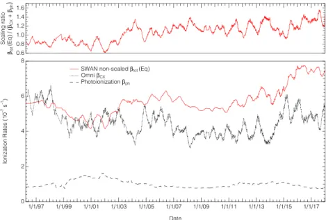
Figure 1 presents the total ionization rate in the equatorial zone derived from the SWAN data analysis as a function of time, compared with proton charge-exchange and photoionization rates. The SWAN total ionization rate represents the sum of charge-exchange and photoionization,
𝛽tot=𝛽CX+𝛽ph. (1)
In Figure 1, 𝛽tot(Eq)is the weighted average of the three near-equatorial latitude bins (0◦, ±10◦) that mostly contribute to the near-ecliptic conditions encountered by L1-orbiting instruments. The proton
Figure 1. Total unscaled ionization rate in the equatorial zone derived from fitting the SWAN Ly-𝛼maps (see details in text; red solid line), along with OMNI CX rates (𝛽CX; black-dotted line) and photoionization rates (𝛽ph; black dashed line) as a function of time. The top panel presents the𝛽tot(Eq)/ (𝛽CX+𝛽ph) ratio, serving as scaling factor (see text). All quantities are running averages over three solar rotations (∼81 days). SWAN = Solar Wind ANisotropy.
charge-exchange rate is calculated with OMNI-2 data from the L1 point according to the simplified equation:
𝛽CX(Vp) =𝜎CX(Vp)npVp(s−1), (2)
where the velocity-dependent cross section is approximated by the Maher and Tinsley (1977) formula and Lindsay and Stebbings (2005) update:
𝜎CX=10−14(1.64 − 0.0695ln(Vp))2 (cm2). (3)
Global photoionization rates are calculated based on CELIAS/SEM data and Lyman-𝛼 time series from LASP, using the empirical formula (2.20) from Bzowski et al. (2013). Electron impact is ignored here, although electron impact rates are approximately half of photoionization rates (Koutroumpa et al., 2012), according to calculations based on quasi-thermal noise data from WIND (Issautier et al., 2005). Future work will include the electron impact following the availability of WIND quasi-thermal noise data.
Up to 2003, the𝛽tot(Eq)/ (𝛽CX+𝛽ph) ratio is stable, although the total SWAN rate is lower than the CX and photoionization sum (see upper panel of Figure 1). Thereafter, there is a progressive drift in the SWAN rates, consistent with the loss of sensitivity mentioned above. To mitigate this change and overcome any residual calibration problems, the SWAN𝛽tot(𝜃) rate for each latitude bin, 𝜃, is scaled by the 𝛽tot(Eq)∕(𝛽CX + 𝛽ph) ratio. In the following sections, all𝛽tot(𝜃) are scaled.
3. SW Flux and Velocity Distributions
From equations (1) and (2) we calculate the proton flux latitude profile Φp(𝜃) = np(𝜃)Vp(𝜃), based on the SWAN𝛽tot(𝜃) ionization rates. We use the IPS velocity measurements from Nagoya University (Tokumaru, 2013) to calculate the velocity-dependent cross sections (from equation (3)) for each latitude bin𝜃. Following that, we use the assumption that dynamic pressure𝜌pVp2or energy flux𝜌pVp(Vp2∕2 + GM⊙∕R⊙) (based on Le Chat et al., 2012), where𝜌pis the proton mass density, are conserved independently from latitude, to calculate the proton speed Vp(𝜃) as a function of latitude 𝜃. Dynamic pressure and energy flux are calculated from the OMNI database, and assuming that they are constant with latitude:
𝜌pVp2=mpΦp(𝜃)Vp(𝜃) = const. (4)
𝜌pVp(Vp2∕2 + GM⊙∕R⊙) =mpΦp(𝜃)(Vp(𝜃)2∕2 + GM⊙∕R⊙) =const. (5) We derive Vp(𝜃) by either equation (4) or (5) by using the SWAN latitude-dependent proton flux Φp(𝜃).
Geophysical Research Letters
10.1029/2019GL082402
Figure 2. From top to bottom, as a function of time: (i) scaled SWAN total ionization rate𝛽tot(𝜃)latitude profiles;
(ii) proton flux npVp(𝜃)latitude profiles, calculated from SWAN ionization rates, and CX cross-sections derived from IPS velocities from equation (2); (iii) velocity latitude profiles, based on SWAN proton fluxes and the dynamic pressure conservation (the profiles derived from the energy flux conservation are very similar); (iv) IPS velocity Vp(𝜃)latitude profiles; (v) coefficient of variation for the latitude-averaged dynamic pressure (black-dotted) and energy flux (red) calculated from the SWAN proton flux and IPS velocities. The two horizontal lines show the standard deviation limits of the coefficients. All panels represent 81-day running averages. Gaps are due to seasonal IPS data gaps, or when SWAN was not operating, as for example in 1998. SWAN = Solar Wind ANisotropy; IPS = Interplanetary Scintillation.
Hydrogen ionization rates, proton flux, and velocity profiles are summarized in Figure 2. We only show the velocity profiles calculated based on the dynamic pressure invariance, as the results based on the energy flux invariance are very similar. We present results up to 70◦latitude because the SWAN fitting procedure is less reliable at higher latitudes. The hydrogen ionization rate pattern (first panel) is reproduced by proton flux profiles (second panel), calculated from equations (2) and (3), using the latitude/velocity-dependent cross-sections (based on IPS data, fourth panel). The main pattern is the difference between minimum and maximum solar phases, but also key differences between the two consecutive solar cycles. A strong anisotropy dominates solar minimum; proton flux is higher at low heliographic latitudes occupied by dense slow SW, where ionization rates are also stronger. Low proton flux (lower ionization rates) dominates higher latitudes where fast wind is less dense. During solar maximum, the SW proton distribution (and subse-quently ionization rates) is more isotropic, but exhibits two peaks at midlatitudes in the north and south hemispheres, also reported in Katushkina et al. (2019). For SC-24, solar activity (proton flux and ionization rate) is overall weaker. The slow SW equatorial zone is more diffuse toward higher latitudes in the 2008 solar minimum. During the SC-24 maximum (2014–2015), the midlatitude peaks are less pronounced and sometimes merged into one asymmetric northern peak. According to Katushkina et al. (2019), the two peaks are related to the expansion of the streamer belt to the poles and the potential presence of equatorial coro-nal holes during maximum. The two-peak evolution in the SC-24 maximum is probably due to north-south asymmetries discovered in the distribution of active regions and coronal holes.
The velocity profiles exhibit similar patterns with proton flux but in reverse scale (highest velocities at higher latitudes where the proton flux is the lowest, and vice-versa for the lower latitudes). The velocity profiles derived from SWAN (based on the dynamic pressure conservation; third panel of Figure 2) show a longer isotropic maximum period during SC-23, that lasts well into 2004–2005, and closely reflect the two
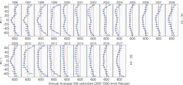
Figure 3. Annual average SW velocity latitude profiles measured with Interplanetary Scintillation (red curves), and
derived from Solar Wind ANisotropy proton fluxes based on dynamic pressure (black dashed curves) and energy flux (blue dotted curves) conservation. The top row corresponds to SC-23, and the bottom to SC-24. SW = solar wind; SC = Solar Cycle.
midlatitude peaks found in the proton flux profiles. The direct IPS measurements (fourth panel) do not show midlatitude peaks, and the maximum period starts earlier, with the latitude isotropy declining faster. Even so, at these timescales (81-day averages) both direct and model-derived velocity profiles exhibit much scatter and conclusions are not easily drawn.
In the last panel of Figure 2 we show the coefficients of variation (𝜎Q∕ < Q >) for the dynamic pressure and energy flux averaged over latitude, calculated from the SWAN proton flux and IPS velocities (second and fourth panels, respectively). Despite noticeable scatter, both quantities are similar in their invariant quality with an average coefficient of variation around 0.23 ± 0.15.
4. Comparison to IPS and Ulysses Velocities
In Figure 3 we compare the annual average velocities, between direct IPS measurements and SWAN-derived values based on the assumption that dynamic pressure and energy flux are invariable quantities. The error-bars for the SWAN-derived values represent the standard deviation from the mean average in the year. SWAN values agree with the direct IPS measurements up to at least ±60◦latitude, for both methods and for gener-ally all solar cycle periods. Both direct IPS and derived SWAN values clearly show the evolution in anisotropy during the solar cycles, with the prominent equatorial zone clearly visible in years 1996–1998 and the change into a more diffuse equatorial zone in 2007–2009. During maximum periods, IPS data are almost perfectly isotropic, while SWAN-derived values exhibit more latitudinal structure, with the midlatitude peaks still prominent, and higher latitude values still showing anisotropy, especially during the SC-23 maximum. Nev-ertheless, we stress again that the SWAN model performance at higher latitudes is less reliable, as explained in the previous sections.
In Figure 4 we draw the comparison with Ulysses in situ measurements at various latitudes. We extracted the SWAN proton flux and velocity for the latitude bins corresponding to Ulysses' latitude and compare with the spacecraft's in situ flux and velocity measurements. We also include OMNI values (energy flux, dynamic pressure, and proton flux) for reference. The gaps in the results correspond to the periods when there is no SWAN or IPS data, as in section 3. The Ulysses data were averaged over 1 solar rotation allowing for a running average that does not overly exceed the 10◦latitude bin size.
In general, both energy flux and dynamic pressure measured by Ulysses and OMNI are fairly consistent, except for a few periods of high solar activity between 2001 and 2006, pinpointed by the arrows in Figure 4 (see specific cases explained below). In all cases where we see a larger discrepancy between the two data sets, the Ulysses data are consistently higher than OMNI.
Geophysical Research Letters
10.1029/2019GL082402
Figure 4. From top to bottom: (i) The top two panels present the Ulysses coordinates (longitude and heliographic
latitude; red), and the Earth/L1 (black-dotted) ecliptic longitude; (ii) OMNI (gray) and Ulysses (red-dotted) energy flux; (iii) OMNI (black) and Ulysses (red-dotted) dynamic pressure; (iv) Ulysses in situ (red-dotted), OMNI in situ (gray) and SWAN-derived (black) proton fluxes; (v) Proton velocities: Ulysses in situ (red-dotted), and SWAN-derived based on energy flux (gray) and dynamic pressure (black) conservation. All in situ data curves (OMNI and Ulysses) are 27-day running averages, while all SWAN curves are 81-day running averages. Notable discrepancies are marked by numbered arrows (see text for details). SWAN = Solar Wind ANisotropy.
The Ulysses and SWAN proton fluxes follow each other remarkably close for most periods, and at all lati-tudes, which gives us confidence over our fitting procedure. The OMNI proton flux is consistent with the other two in solar maximum periods at all latitudes, and in solar minimum when Ulysses and SWAN data correspond to low latitude bins. At low activity periods, when Ulysses and SWAN scan high latitude bins (1996 to early 1997, 2006 to early 2007, and after 2008), the OMNI flux is consistently higher, since the database represents the low latitude high density slow SW. We stress again, that the SWAN proton flux is calculated independently of the OMNI data, except for a normalization to correct for SWAN's sensitivity drift.
The general evolution in the Ulysses in situ velocities is well reproduced by the SWAN analysis, although when discrepancies occur, they are in general more extreme than in the case of proton flux. However, in the velocity calculations, we also introduce the OMNI data set by using the energy flux and dynamic pressure conservation hypotheses. In the absence of notable variations in the OMNI (and Ulysses) dynamic pressure, or energy flux, as is the case during quiet periods in solar minimum in 1997–1998, and 2007, Ulysses and SWAN are in excellent agreement for both the proton flux and speed, up to the highest latitudes. When there are substantial differences in the proton flux or velocity values, we can identify four specific cases: 1. In two cases the SWAN proton flux drops suddenly and subsequently the SWAN-derived velocity is
consid-erably higher with respect to Ulysses. In both cases, the energy flux and dynamic pressure are consistent between OMNI and Ulysses. The first case occurs in the weeks following the Bastille Day solar storm in July 2000, and the second one in December 2007 with no equivalent solar event recorded. A quick review of the SWAN maps reveals considerable saturation in the first case only. In addition, the SWAN values correspond to high latitude bins (−70◦and +70◦, respectively) where the fitting procedure becomes less reliable. We thus conclude that these discrepancies are due to the SWAN fit results, although there were no red-flags in the model fit filter criteria.
2. In the period between mid-2001 up to late 2002, Ulysses measured energy fluxes and dynamic pressures notably higher than OMNI, while the SWAN-derived proton flux was slightly higher than the one mea-sured in situ by Ulysses. In this case, the velocity results are considerably different between SWAN and Ulysses. This may be attributed to the fact that Ulysses and OMNI were sounding different SW streams, as the former is rarely in close conjunction with the L1 orbiting instruments. To calculate the SWAN velocity
as a function of latitude we use the OMNI energy flux and dynamic pressure, hence the discrepancy we find with the Ulysses measured velocities.
3. In reverse, on one occasion in late 2003 when both Ulysses invariants are higher than the OMNI ones, and the SWAN proton flux is considerably lower than measured with Ulysses, then the results even out to produce a perfect match between Ulysses and SWAN velocity values. The OMNI proton flux is very close to the SWAN value as we sound the low latitude bins, but Ulysses seems to scan higher proton fluxes and is in general in a different longitude quadrant. Therefore, in that case, the velocity agreement may be purely coincidental for two streams with different densities.
4. Finally, discrepancies between the invariants measured by OMNI and Ulysses (in the years 2005–2006), with no apparent discrepancy between the SWAN and Ulysses proton fluxes, will still produce a differ-ence in the velocity values. In this case too, we argue that OMNI and Ulysses were sounding different SW streams, which reflects upon the velocity calculation based on energy flux and dynamic pressure conservation.
5. Summary and Conclusions
We have analyzed over 4,000 backscattered Ly-𝛼 maps recorded with SWAN for 22 years, covering two solar cycles. We derived the latitudinal profile of the total ionization rate for interplanetary hydrogen as a func-tion of time, and confirmed previous findings on the temporal evolufunc-tion of the SW distribufunc-tion for SC-23 and SC-24, notably the two midlatitude peaks during solar maximum and a much weaker activity during SC-24 with a considerably larger equatorial zone during solar minimum in the later cycle. The hydrogen ionization rates closely reflect the proton flux 3-D distribution, and we were able to calculate the proton flux latitudinal profile aided by the latitude/velocity-dependent cross section calculated with the IPS velocities at all latitudes.
From the SWAN proton fluxes we also calculated the velocity latitude profiles as a function of time based on the assumptions that dynamic pressure and energy flux (both calculated with OMNI data) are invariable over latitude. The two methods give very similar results that we compared with annual averages of the SW velocity profiles from IPS observations, and with in situ measurements from Ulysses at various latitudes. Overall, the results prove that the SWAN-derived SW distribution is in good agreement with the conservation of the two invariable quantities equally.
The annual average velocities derived from SWAN are in very good agreement within the errorbars with direct IPS measurements, in most cases up to at least ±60◦latitude. Larger discrepancies occur at higher latitudes (in particular for the couple of years preceding solar maxima) for reasons currently unknown. Although the SWAN fitting procedure is less reliable at those latitudes, the discrepancies are not necessar-ily explained by the various tests and criteria applied on the quality of the fits. Finally, compared to in situ Ulysses measurements at various latitudes, the SWAN-derived fluxes and velocities follow relatively closely the in situ data trends up to at least ±60◦, particularly during periods of quiet solar activity (1997–1998 and 2007), where there are no notable eruptive perturbations in the ecliptic (OMNI) and high-latitude (Ulysses) measurements. Large discrepancies are more frequent during strong solar activity and especially at higher latitudes. This is partly due to the SWAN fitting bias at high latitudes, or to the fact that OMNI (used to calcu-late the energy flux and dynamic pressure) and Ulysses probably reflect different in situ SW measurements, while SWAN reflects global conditions in the heliosphere.
Future work will involve an updated analysis of the SWAN absolute calibration and a systematic examination of the SWAN fitting bias at high latitudes. We are also working into including estimates for the electron impact ionization rate from quasi-thermal noise data from WIND.
References
Baliukin, I. I., Bertaux, J., Quémerais, E., Izmodenov, V. V., & Schmidt, W. (2019). SWAN/SOHO Lyman-𝛼mapping: The hydrogen geocorona extends well beyond the Moon. Journal of Geophysical Research: Space Physics, 124, 861–885. https://doi.org/10.1029/ 2018JA026136
Bertaux, J. L., Kyrölä, E., Quémerais, E., Pellinen, R., Lallement, R., Schmidt, W., & Holzer, T. (1995). SWAN: A study of solar wind anisotropies on SOHO with Lyman𝛼sky mapping. Solar Physics, 162(1-2), 403–439. https://doi.org/10.1007/BF00733435
Bzowski, M., Sokol, J. M., Tokumaru, M., Fujiki, K., Quémerais, E., Lallement, R., & McComas, D. J. (2013). Solar parameters for modeling interplanetary background. In Cross-calibration of far UV spectra of solar system objects and the heliosphere ISSI scientific report series (Vol. 13, pp. 67). New York: Springer Science+Business Media. https://doi.org/10.1007/978-1-4614-6384-9_3
Acknowledgments
This work was supported by the CNES. It is based on observations with SWAN embarked on SOHO. SOHO is a mission of cooperation between ESA and NASA. SWAN was developed as a cooperation between France (CNRS, CNES) and Finland (Finnish Meteorological Institute). The SWAN full-sky maps are available online (at http://swan.projet.latmos.ipsl.fr/). The SWAN inversion simulations were performed at the High Performance Computer and Visualisation platform (HPCaVe) hosted by UPMC-Sorbonne Universités. The OMNI-2 and Ulysses data were retrieved from NASA's GSFC Space Physics Data Facility (at https://spdf.gsfc.nasa.gov/). The IPS velocity data were retrieved from the Institute for Space-Earth Environmental Research (ISEE) of Nagoya University (at http://stsw1. isee.nagoya-u.ac.jp/
Geophysical Research Letters
10.1029/2019GL082402
Clarke, J. T., Lallement, R., Bertaux, J. L., Fahr, H., Quémerais, E., & Scherer, H. (1998). HST /GHRS observations of the velocity structure of interplanetary hydrogen. The Astrophysical Journal, 499(1), 482–488. https://doi.org/10.1086/305628
Issautier, K., Perche, C., Hoang, S., Lacombe, C., Maksimovic, M., Bougeret, J. L., & Salem, C. (2005). Solar wind electron density and temperature over solar cycle 23: Thermal noise measurements on Wind. Advances in Space Research, 35(12), 2141–2146. https://doi.org/ 10.1016/j.asr.2005.04.085
Joselyn, J. A., & Holzer, T. E. (1975). The effect of asymmetric solar wind on the Lyman𝛼sky background. Journal of Geophysical Research,
80(7), 903–907. https://doi.org/10.1029/JA080i007p00903
Katushkina, O., Izmodenov, V., Koutroumpa, D., Quémerais, E., & Jian, L. K. (2019). Unexpected behavior of the solar wind mass flux during solar maxima: Two peaks at middle heliolatitudes. Solar Physics, 294(2), 17. https://doi.org/10.1007/s11207-018-1391-5 King, J. H., & Papitashvili, N. E. (2005). Solar wind spatial scales in and comparisons of hourly Wind and ACE plasma and magnetic field
data. Journal of Geophysical Research, 110, A02104. https://doi.org/10.1029/2004JA010649
Koutroumpa, D., Quémerais, E., Lallement, R., Ferron, S., & Bertaux, J. L. (2012). Time and latitude dependence of the solar wind mass flux derived from the SOHO/SWAN data analysis. American Geophysical Union, Fall Meeting 2012, abstract id.SH13C-2275. Lallement, R., Bertaux, J. L., & Kurt, V. G. (1985). Solar wind decrease at high heliographic latitudes detected from Prognoz interplanetary
lyman alpha mapping. Journal of Geophysical Research, 90(A2), 1413. https://doi.org/10.1029/JA090iA02p01413
Le Chat, G., Issautier, K., & Meyer-Vernet, N. (2012). The solar wind energy flux. Solar Physics, 279(1), 197–205. https://doi.org/10.1007/ s11207-012-9967-y
Lindsay, B. G., & Stebbings, R. F. (2005). Charge transfer cross sections for energetic neutral atom data analysis. Journal of Geophysical
Research, 110, A12213. https://doi.org/10.1029/2005JA011298
Maher, L. J., & Tinsley, B. A. (1977). Atomic hydrogen escape rate due to charge exchange with hot plasmaspheric ions. Journal of
Geophysical Research, 82(4), 689. https://doi.org/10.1029/JA082i004p00689
Marsch, E., & Richter, A. K. (1984). Helios observational constraints on solar wind expansion. Journal of Geophysical Research, 89(A8), 6599. https://doi.org/10.1029/JA089iA08p06599
McComas, D. J., Angold, N., Elliott, H. A., Livadiotis, G., Schwadron, N. A., Skoug, R. M., & Smith, C. W. (2013). Weakest solar wind of the space age and the current “mini” solar maximum. The Astrophysical Journal, 779(1), 2. https://doi.org/10.1088/0004-637X/779/1/2 Quémerais, E., Bertaux, J. L., Lallement, R., Berthé, M., Kyrölä, E., & Schmidt, W. (1999). Interplanetary Lyman𝛼line profiles derived from
SWAN/SOHO hydrogen cell measurements: Full-sky velocity field. Journal of Geophysical Research, 104(A6), 12,585. https://doi.org/ 10.1029/1998JA900101
Quémerais, E., Lallement, R., Ferron, S., Koutroumpa, D., Bertaux, J. L., Kyrölä, E., & Schmidt, W. (2006). Interplanetary hydrogen absolute ionization rates: Retrieving the solar wind mass flux latitude and cycle dependence with SWAN/SOHO maps. Journal of Geophysical
Research, 111, A09114. https://doi.org/10.1029/2006JA011711
Quémerais, E., Sandel, B. R., Izmodenov, V. V., & Gladstone, G. R. (2013). Thirty years of interplanetary background data: A global view,
Cross-calibration of far UV spectra of solar system objects and the heliosphere(Vol. 13, pp. 141–162). New York, NY: Springer New York. https://doi.org/10.1007/978-1-4614-6384-9_4
Richardson, J., & Wang, C. (1999). The global nature of solar cycle variations of the solar wind dynamic pressure. Geophysical Research
Letters, 26(5), 561–564. https://doi.org/10.1029/1999GL900052
Rosenbauer, H., Schwenn, R., Marsch, E., Meyer, B., Miggenrieder, H., Montgomery, M. D., & Zink, S. M. (1977). A survey on initial results of the HELIOS plasma experiment. Journal of Geophysics - Zeitschrift für Geophysik, 42(6), 561–580. NASA-supported research; Bundesministerium für Forschung und Technologie.
Schwenn, R., Mohlhauser, K. H., & Rosenbauer, H. (1981). Two states of the solar wind at the time of solar activity minimum—Part one—Boundary layers between fast and slow streams. In H. Rosenbauer (Ed.), Solar wind 4, proceedings of the conferene held in
August 18-September 1, 1978 in Burghausen, FDR(pp. 118). Burghausen: MPAE-W-100-81-31. Garching, FDR: Max-Planck-Institute für Aeronomie. http://adsabs.harvard.edu/abs/1981sowi.conf..118S
Tokumaru, M. (2013). Three-dimensional exploration of the solar wind using observations of interplanetary scintillation. Proceedings of