RESEARCH OUTPUTS / RÉSULTATS DE RECHERCHE
Author(s) - Auteur(s) :
Publication date - Date de publication :
Permanent link - Permalien :
Rights / License - Licence de droit d’auteur :
Bibliothèque Universitaire Moretus Plantin
Institutional Repository - Research Portal
Dépôt Institutionnel - Portail de la Recherche
researchportal.unamur.be
University of Namur
Biodiversity effects on ecosystem functioning respond unimodally to environmental
stress
Baert, Jan; Eisenhauer, Nico; JANSSEN, C.; De Laender, Frédérik
Published in:
Ecology Letters
DOI:
10.1111/ele.13088
Publication date:
2018
Document Version
Peer reviewed version
Link to publication
Citation for pulished version (HARVARD):
Baert, J, Eisenhauer, N, JANSSEN, C & De Laender, F 2018, 'Biodiversity effects on ecosystem functioning
respond unimodally to environmental stress', Ecology Letters, vol. 21, no. 8, pp. 1191-1199.
https://doi.org/10.1111/ele.13088
General rights
Copyright and moral rights for the publications made accessible in the public portal are retained by the authors and/or other copyright owners and it is a condition of accessing publications that users recognise and abide by the legal requirements associated with these rights. • Users may download and print one copy of any publication from the public portal for the purpose of private study or research. • You may not further distribute the material or use it for any profit-making activity or commercial gain
• You may freely distribute the URL identifying the publication in the public portal ?
Take down policy
If you believe that this document breaches copyright please contact us providing details, and we will remove access to the work immediately and investigate your claim.
Biodiversity effects on ecosystem functioning respond unimodal to
1
environmental stress
2
Baert Jan M.1,2*, Eisenhauer Nico3,4, Janssen Colin R.1 and De Laender Frederik5
3
1 Laboratory of Environmental Toxicology and Applied Ecology, Ghent University, Coupure Links
4
653, 9000 Ghent, Belgium 5
2 Ethology (ETHO), University of Antwerp, Universiteitsplein 1, 2610 Antwerp, Belgium
6
3 German Centre for Integrative Biodiversity Research (iDiv) Halle-Jena-Leipzig, Deutscher Platz
7
5e, 04103 Leipzig, Germany 8
4 Institute of Biology, Leipzig University, Deutscher Platz 5e, 04103 Leipzig, Germany
9
5 Institute of Life-Earth-Environment, Namur Institute of Complex Systems, Research Unit of
10
Environmental and Evolutionary Biology, University of Namur, Rue de Bruxelles 61, 5000 11
Namur, Belgium 12
* Corresponding author e: [email protected] t: +32 9264 3767 13
Author contributions
14
JMB and FDL conceived the idea. JMB implemented the model and analysed the data. JMB, NE, CRJ
15
and FDL contributed to discussions and wrote the manuscript.
16 17
Data accessibility statement
18
References for all studies used in the meta-analyses with detailed descriptions of the source of the
19
data are given in Table S1.
20 21 Manuscript info 22 Type: Letter 23 Abstract: 150 words 24 Text: 4026 words 25 Figures: 4 26
Tables: 1
27
Abstract
28
Understanding how biodiversity (B) affects ecosystem functioning (EF) is essential for assessing the
29
consequences of ongoing biodiversity changes. An increasing number of studies, however, shows that
30
environmental conditions affect the shape of BEF relationships. Here, we first use a game-theoretic
31
community model to reveal that a unimodal response of the BEF slope can be expected along
32
environmental stress gradients, but also that the ecological mechanisms underlying this response may
33
vary depending on how stress affects species interactions. Next, we analyzed a global dataset of 44
34
experiments that crossed biodiversity with environmental conditions, confirming our main model
35
predictions: the effect of biodiversity on ecosystem functioning is greater at intermediate levels of
36
environmental stress, but this effect varies considerably among studies depending on the type of
37
species interactions. Together, these results suggest that increases in stress from ongoing global
38
environmental changes may amplify the consequences of future biodiversity changes.
39 40
41 42 43 44 45 46 47 48 49 50 51 52 53
Introduction
54
Over the past 25 years, a compelling number of experiments has demonstrated that biodiversity
55
affects ecosystem functioning (Chapin et al. 1997; Loreau et al. 2001; Hooper et al. 2005; Cardinale et
56
al. 2011, 2012). Since most studies support a positive biodiversity-ecosystem functioning (BEF)
57
relationship, this has raised concerns that ecosystem function provisioning is at risk from ongoing
58
global biodiversity changes (Hooper et al. 2005, 2012; Cardinale et al. 2012). However, evidence is also
59
mounting that the consequences of biodiversity changes may not be predictable from a single,
60
universal BEF relationship (Mittelbach et al. 2001; Pärtel et al. 2010; Tilman et al. 2014). Not only can
61
the shape of BEF relationships differ among ecosystems (Cardinale et al. 2011, 2012), an increasing
62
number of studies now demonstrates that changes in environmental conditions can also alter the
63
shape of BEF relationships within a system (Pfisterer & Schmidtke 2002; Wardle & Zackrisson 2005; Li
64
et al. 2010; Steudel et al. 2011, 2012; Isbell et al. 2015; Baert et al. 2016; Guerrero-Ramírez et al. 2017).
65
How environmental changes alter the shape of the BEF relationship thereby appears to strongly
66
depend on both the system and environmental change driver under study (Cowles et al. 2016; Ratcliffe
67
et al. 2017). However, few studies have so far explored the processes underlying observed
68
environmental change-induced alterations in BEF relationships (Rixen & Mulder 2005; Baert et al.
69
2016; Hodapp et al. 2016). Hence, it remains unstudied if differences among studies in how
70
environmental changes alter BEF relationships can be reconciled within a single mechanistic
71
framework. This is a major knowledge gap as observations and prognoses suggest rapid future changes
72
in environmental conditions to go hand in hand with biodiversity change, which can cause the
73
consequences of predicted biodiversity changes to deviate from the current expectations that are
74
based on the current-day environmental conditions (Pereira et al. 2010; Sala et al. 2011; Hooper et al.
75
2012; Pimm et al. 2014).
76 77
Biodiversity research has thus far mostly focused on aggregated ecosystem functions (e.g. total
78
biomass production) in single trophic level systems (Hooper et al. 2005; Tilman et al. 2014; Ratcliffe et
al. 2017). Such ecosystem functions typically consist of the sum of the individual species’ functional
80
contributions. Biodiversity effects on aggregated ecosystem functions therefore result from
81
differences in the relative strength of inter- and intraspecific interactions, which cause species to
82
function differently in the presence of other species (Loreau & Hector 2001; Fox 2005). Two classes of
83
biodiversity effects are thereby discerned: dominance and complementarity effects (Loreau & Hector
84
2001; Fox 2005). Dominance effects refer to changes in ecosystem functions through changes in
85
species’ functional contributions as a result of competitive replacement, and hence increase
86
ecosystem functioning when functional and competitive abilities are correlated so that
high-87
functioning species replace low-functioning species. Complementarity effects, in contrast, refer to
88
changes in species functional contributions by alterations in the amount of competition through the
89
presence of heterospecifics, but without resulting in competitive replacement. Niche complementarity
90
and facilitation are hence two important drivers of positive complementarity effects, increasing
91
species’ functioning by reducing the amount of competition individuals experience in mixed
92
communities compared to monocultures (Loreau & Hector 2001; Mulder et al. 2001; Fox 2005). A
93
distinction can thereby be made between trait-independent and trait-dependent complementarity
94
effects. Trait-independent complementarity effects refer to the average complementarity effect
95
across species as a result of all interactions in the system. Trait-dependent complementarity effects
96
designate how species deviate from this average complementarity effect in relation to their functional
97
traits, generally quantified as their monoculture yield, as a result of asymmetric or one-way
98
interactions. Both classes of biodiversity effects can also be negative. Dominance of species with low
99
functional abilities and antagonistic interactions that increase competition can accordingly result in
100
negative dominance and complementarity effects, respectively, and thus in negative BEF relationships
101
(Loreau & Hector 2001; Fox 2005).
102 103
Theoretically, the environmental dependency of BEF relationships should thus arise from changes in
104
species functional contributions that alter dominance and complementarity effects (Baert et al. 2016).
Environmental change can affect species functional contributions directly and indirectly. Interspecific
106
differences in species’ sensitivities to the environmental changes determine direct effects. Species
107
interactions may cause additional indirect effects by changing the density of a species’ competitors
108
(May 1974; Mccann et al. 1998; Ives et al. 1999). Opposing ecological theories exist, however, on the
109
effect of environmental stress on these species interactions themselves, assuming the per-capita to
110
either remain unaffected, change in strength, or even shift from competitive to facilitation at high
111
stress (Chesson & Huntly 1997; Hart & Marshall 2013). The importance of environmental stress effects
112
on species interactions for biodiversity effects on function remains unresolved at present (Baert et al.
113
2016).
114 115
Environmental stress invariably selects for tolerant species. We therefore hypothesize that the slope
116
of BEF relationships should initially increase with environmental stress. Biodiversity increases the
117
probability that a system will contain tolerant species that can replace sensitive species (in line with
118
the insurance effect of biodiversity, Yachi & Loreau 1999). Hence, more diverse systems are less likely
119
to experience severe reductions in function compared to less diverse systems, resulting in an increased
120
slope of BEF relationships (Steudel et al. 2012; Hodapp et al. 2016). However, the BEF relationship
121
should collapse to a horizontal line when stress is sufficiently high to inhibit the growth of all species.
122
Thus, overall, the slope of a BEF relationship should respond to stress in a unimodal way. Moreover,
123
stress inevitably induces a correlation between functional and competitive abilities, causing tolerant
124
species that grow relatively well in monoculture to displace sensitive species as stress intensifies (Baert
125
et al. 2016). Hence, we expect that the response of the dominance effect to stress will be the key driver
126
of this unimodal response.
127 128
Here, we first used a game theoretic competition model to explore how increasing environmental
129
stress alters BEF relationships for aggregated ecosystem functions and the underlying dominance and
130
complementarity effects in competitive systems. We simulated four different scenarios of
environmental stress effects on per-capita interactions: environmental stress had either no effect,
132
increased, or decreased the strength of per-capita interactions without changing the type of species
133
interactions, or reduced per-capita interactions with obligate shifts to complementarity at high levels
134
of environmental stress as postulated by the stress gradient hypothesis (REF). Direct effects of
135
environmental stress on fitness were modelled as reductions in species per-capita growth rates in all
136
scenarios. We tested if BEF-relationships and underlying biodiversity effects responded monotonically
137
or unimodally to increasing environmental stress, by fitting second order polynomials to the simulated
138
data. To assess the generality of our findings, we performed this analysis for a wide range of BEF
139
relationships that are theoretically possible under unstressed conditions, including negative,
140
horizontal, and positive BEF relationships. Next, we confronted model predictions with observed
141
changes in BEF relationships from a meta-analysis of 44 studies in primary producer systems that
142
manipulated species richness under at least 3 different environmental conditions.
143 144
Methods
145 Model structure 146We used a stochastic game theoretic community model (Huang et al. 2015) to simulate a broad
147
spectrum of theoretically possible BEF relationships. In this model, population dynamics are thereby
148
assumed to be exclusively driven by birth, death, and inter- and intraspecific interaction processes,
149
occurring at rates b, d and a, respectively. For every species i, the rates at which its density (Ni) may
150
increase (Ti+) or decrease (Ti-) by one individual can be expressed as:
151
𝑇𝑖+= 𝑏𝑖 𝑁𝑖 (eq. 1), 152
𝑇𝑖−= 𝑑𝑖 𝑁𝑖+ 𝑁𝑖∑𝑛𝑗=1𝑎𝑖,𝑗 𝑁𝑗 (eq. 2), 153
where n is the number of species in the community. In the absence of heterospecifics (i.e. n=1), the
154
equilibrium density of species i thereby equals 𝑎𝑖,𝑖−1 (𝑏𝑖− 𝑑𝑖). Note that, as birth and death events 155
are independent, stochastic demographic fluctuations will occur around the equilibrium population
156
density in the system (Huang et al. 2015).
157
We consider a one-dimensional environmental gradient (E) along which species functioning is altered
158
through direct effects on the per-capita growth rate (Fig. 1). The species-specific functional response,
159
ri(E), was modelled by a normalised gamma distribution to restrict values between 0 and 1 (i.e.
160
maximal fitness; Fig. 1):
161 𝑟𝑖(𝐸) = [ 𝐸 𝜃𝑖 (𝑘𝑖−1)] 𝑘𝑖−1 𝑒− 𝐸 𝜃𝑖+(𝑘𝑖−1) (eq. 4). 162
The shape parameter ki and scale parameter θi of the gamma distribution thus determine the width
163
of the environmental niche (~ki θi2) and the optimal environmental conditions (ki θi) at which the
164
maximal per-capita birth rate of species i is attained. We used a gamma distribution to allow for both
165
symmetrical and asymmetrical niches. Note that values for the environmental gradient are hence
166
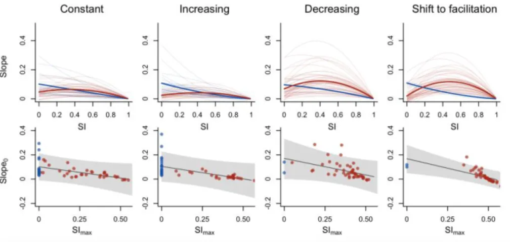
restricted to positive values.
167
The per-capita growth rate of each species along the environmental gradients bi(E) can hence be
168
written as:
169
𝑏𝑖(𝐸) = 𝑏0,𝑖 𝑟𝑖(𝐸) (eq. 3), 170
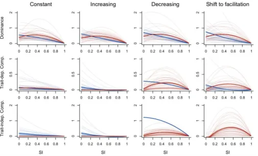
where b0,i is the maximal per-capita birth rate of species i at optimal environmental conditions (Fig.
171
1).
172 173
Since optimal conditions and functional responses may differ among species within a system, we
174
quantify the stressfulness of environmental conditions (E) as the stress intensity (SI), which is the
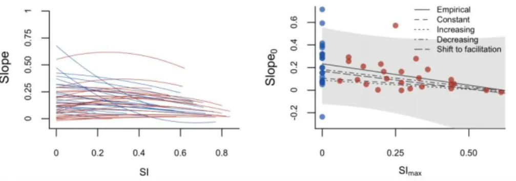
175
average species’ fitness reduction at these environmental conditions (Steudel et al. 2012):
176 𝑆𝐼(𝐸) = 1 − ∑ 𝑟𝑘(𝐸) 𝑚 𝑚 𝑘=1 (eq. 5), 177
where m is the number or species within the experiment (see also model simulations). Hence, stress
178
intensity ranged from 0 for on average optimal conditions to 1 for severely stressed conditions (Fig. 1).
We define four scenarios of environmental stress effects on per-capita interactions, representing the
180
main hypotheses commonly postulated (Hart & Marshall 2013). When the type of species interactions
181
is not altered by stress, stress effects on per-capita interactions are modelled as:
182
𝑎𝑖,𝑗(𝐸) = 𝑎0,𝑖,𝑗 [1 + 𝛽𝑖 𝑆𝐼(𝐸)]𝛾 (eq. 6). 183
The species-specific parameter 𝛽𝑖 thereby denotes the strength by increasing environmental stress 184
affects per-capita interactions for a given species. The power γ defines whether per capita interactions
185
are unaffected (γ=0; scenario 1), increase (γ=1; scenario 2) or decrease (γ=-1; scenario 4) with
186
increasing stress. For the fourth scenario in which per capita interactions shift to facilitation by
187
environmental stress, i.e. change sign as proposed by the stress gradient hypothesis (Maestre et al.
188
2009), stress effects on per-capita interactions are modelled as:
189
𝑎𝑖,𝑗(𝐸) = 𝑎0,𝑖,𝑗 [𝑐𝑖− 𝑆𝐼(𝐸)][1 + 𝛽𝑖 𝑆𝐼(𝐸)]𝛾 (eq. 7), 190
where the species-specific parameter ci indicates the stress intensity at which per capita interactions
191
for species i become negative, and thus shift from competition to facilitation.
192 193
Along the one-dimensional environmental gradient, the transition rates of a system of n species under
194
given environmental conditions (E) can thus be written as:
195 𝑇𝑖+= 𝑏 𝑖(𝐸) 𝑁𝑖 (eq. 8), 196 𝑇𝑖−= 𝑑 𝑖 𝑁𝑖+ 𝑁𝑖∑𝑛𝑗=1𝑎𝑖,𝑗(𝐸) 𝑁𝑗 (eq.9). 197 198
Scenarios and parameterisation
199
We simulated the model for four scenarios of environmental stress on per-capita interactions. In the
200
first scenario, we assumed no effects of environmental stress on per-capita interactions. Hence, the
201
parameter γ was set to zero for those model simulations (eq. 6). In the second and third scenario, we
202
assumed a continuous increase or decrease in per-capita interactions, and thus competition, but
203
without changes in the type of interactions at high stress (eq. 6). In both scenarios, 𝛽𝑖 was sampled 204
from U(0, 10) for each model simulation. The parameter γ was set to 1 (scenario 2) or -1 (scenario 3)
to simulate a continuous increase or decrease strength of per-capita interactions, respectively. In the
206
fourth scenario, we assumed a linear decrease in per-capita interactions with shifts to facilitation at
207
high levels of environmental stress (eq. 7). Identical to scenario 3, 𝛽𝑖 was sampled from U(0, 10) and 208
γ was set to -1. The additional parameter ci, denoting the stress intensity at which per-capita
209
interactions shift from positive to negative, was sampled from U(0.75, 1) for each model simulation.
210 211
We used a Monte-Carlo simulation procedure to generate 100 BEF relationships, and simulated
212
changes in each of those BEF relationships by increasing environmental stress, for each of the four
213
scenarios of environmental stress effects on per-capita interactions. The generated set of BEF
214
relationships represented an exhaustive set of ecologically relevant BEF relationships under unstressed
215
conditions, ranging from negative to strongly positive relationships (Fig. 2). Per capita birth rates under
216
optimal conditions, b0,i, and per capita mortality rates, di, were randomly sampled from U(0, 1) and 217
U(0, 0.01b0,i), respectively. The means of the gamma distributions (i.e. the optimal environmental
218
conditions for every species), were sampled from U(95, 105), and the variances were sampled from
219
U(10, 50). The strength of intraspecific interactions ai,i,, which is the main determinant of differences
220
among species monoculture yields, was sampled from U(10-4,10-3). The strength of interspecific
221
interactions was subsequently sampled from U(-0.01 ai,i ,2 ai,i). A sensitivity analysis of the parameters
222
distributions revealed that the model results did not depend on the parameter distributions: using
223
different sets of ecologically relevant parameter distributions did not alter our results (Fig. S1).
224 225
Model simulations
226
For each simulation, we first generated a pool of 20 species by randomly drawing values for b0,i, ki, θi,
227
di, αi,i and αi,j for all species (Fig. S2). Next, 10 communities of 2, 4, 8, and 16 species were randomly
228
assembled from this species pool, representing a standard design used in BEF studies ). Community
229
dynamics were then simulated under unstressed conditions and under nine conditions of
230
environmental stress intensity (SI=0.1, 0.2, 0.3, 0.4, 0.5, 0.6, 0.7, 0.8, 0.9; Fig. S2). Community dynamics
were simulated using the Gillespie algorithm to shorten simulation times by optimizing the length of
232
the time-steps used (Gillespie 1976). Initial (t=0) densities were set to 100 for all species. Population
233
densities always reached their stationary distribution at t≤30. Simulations were run till t=50. Mean
234
species densities were calculated from the species densities between t=40 and t=50. Each simulation
235
was reiterated 12 times to ensure convergence of the stationary distribution (Fig. S3).
236 237
Ecosystem functioning was calculated as the sum of the mean species’ densities. BEF relationships at
238
each level of environmental stress were subsequently calculated by linearly regressing functioning
239
against the initial species richness of the system. Biodiversity effects for all environmental conditions
240
were calculated according to the additive partitioning approach by Fox (Fox 2005):
241 ∆𝑌 = ∑ 𝑌𝑛 𝑜,𝑖− 𝑌𝑒,𝑖 𝑖 = ∑ (𝑅𝑌𝑛𝑖 𝑜,𝑖− 𝑅𝑌𝑒,𝑖)𝑀𝑖= 𝑛 𝑐𝑜𝑣 ( 𝑅𝑌𝑜,𝑖 𝑅𝑌𝑇− 𝑅𝑌𝑒,𝑖, 𝑀𝑖) + 𝑐𝑜𝑣 (𝑅𝑌𝑜,𝑖− 𝑅𝑌𝑜,𝑖 𝑅𝑌𝑇, 𝑀𝑖) + 242 𝑛 𝐸(∆𝑅𝑌)𝐸(𝑀) (eq.10), 243
where ΔY is the deviation between the expected and observed yield, which is the sum of the individual
244
species deviations between observed (Yo,i) and expected yields (Ye,i). RY denotes the relative yield, i.e.
245
the fraction of the monoculture yield. The expected relative yield (RYe,i) thereby equals the species
246
initial proportion in the mixture (i.e. n-1), whereas the observed relative yield is the mean value of each
247
species stationary distribution divided by its monoculture yield under the same environmental
248
conditions (𝑀𝑖= 𝑎𝑖,𝑖 [𝑏𝑖(𝐸𝑛𝑣) − 𝑑𝑖]). RYT is the relative yield total (i.e. ∑ 𝑅𝑌𝑛𝑖 𝑜,𝑖). 249
250
Review of literature data
251
We searched Thomas Reuters Web of Knowledge (www.webofknowledge.com) and Google Scholar
252
(www.scholar.google.com) in February 2018 for experiments that manipulated species richness under
253
at least three environmental conditions. We used the search terms “biodiversity”, “ecosystem”,
254
“function”, “productivity”, “stress”, “temperature”, “nutrient”, “precipitation”, “chemical”, “salinity”,
255
“environment” in various combinations. We additionally checked the cited literature for further
256
original studies. Data were available as text, excel files or were digitized from the figures in the original
publications. Digitized data did not differ by more than 1% among different applications (e.g. Engauge,
258
WebPlot, ExtractGraph digitizer). When slopes and intercepts of BEF relationships were not reported,
259
these were calculated from the data. Only studies that manipulated biodiversity under at least three
260
environmental conditions, and reported the species monoculture functions for all environmental
261
conditions were considered, as this is a prerequisite to calculate the intensity of environmental stress
262
and discriminate between monotonic and unimodal changes in BEF relationships (see Data
263
normalisation and analysis). This yielded a total of 44 studies (Fig. S4, Table S1), all of which used
264
primary producer systems. Environmental gradients comprised drought (n=37), temperature (n=3),
265
pollutants (n=2), salt (n=1), nutrients (n=1) and shade (n=1).
266 267
Data normalisation
268
Literature and simulated data were normalized prior to analysis. The severity of the environmental
269
stress was calculated, analogous to model simulations (eq. 5), as the ratio between the average
270
observed monoculture under stress and unstressed conditions for all species in the study. Unstressed
271
conditions were defined as those environmental conditions under which species attained the highest
272
mean monoculture functions. Since the units in which aggregated ecosystem functions are measured
273
varied among studies, slopes were normalized by dividing the linear regression coefficient of the BEF
274
relationship by the average monoculture function under unstressed conditions. Thus, normalised
275
slopes all had species-1 as a unit.
276 277
Analysis of simulated and empirical data
278
We carried out the same analyses on the simulated data (including all four scenarios of environmental
279
effects on per-capita interactions) as on the empirical data. First, we tested how the slope of BEF
280
relationships changed along environmental stress gradients using second order polynomials. Next, we
281
tested how the effect on the BEF slope varied among the range of unstressed BEF relationships
282
considered by the model or present in the empirical data. To do so, we regressed the slope under
unstressed conditions against the stress intensity at which the BEF slope peaked. The dataset ID (i.e.
284
simulated scenario 1, 2, 3, and 4? or empirical data) was included as an additional factorial fixed effect
285
in the linear regression model to be able to compare among simulated scenarios and between
286
simulations and empirical data. Residual diagnostics were assessed for deviations from normality and
287 homoscedasticity (Fig. S5). 288 289
Results
290 Model simulations 291Model simulations revealed highly consistent changes in the slope of BEF relationships, irrespective of
292
how environmental stress affected per-capita interactions (Fig. 2). In all four scenarios, most
293
simulations confirmed a unimodal response of the slope of the BEF relationship to increasing
294
environmental stress: biodiversity effects peaked at intermediate levels of environmental stress (Fig.
295
2). Only when initial BEF slopes were high, the model predicted a monotonic decrease in BEF
296
relationships. When synthesising across the wide range of BEF relationships under unstressed
297
conditions considered by our modelling, we found a negative relationship between the slope under
298
unstressed conditions and the level of environmental stress where the BEF slope peaks (Fig. 2).
299 300
While BEF relationships responded consistently to environmental stress across all simulations, the
301
responses of the underlying biodiversity effects, however, depended strongly on how per-capita
302
interactions were affected by environmental stress. In all four scenarios, environmental stress-induced
303
changes in dominance effects drove the change in BEF relationships (Fig. 3). Unimodal changes in the
304
complementarity effects, in contrast, only contributed to overall changes of the BEF relationship in
305
scenarios 3 and 4, where the strength of per-capita interactions decreased with increasing
306
environmental stress. When per-capita interactions remained constant or increased with
307
environmental stress, complementarity effects instead on average decreased monotonically.
308 309
Meta-analysis of biodiversity experiments
310
Observed responses of the slope of BEF relationships to environmental stress, as reported in the 44
311
empirical studies, confirm predictions of a predominantly unimodal model response of BEF
312
relationships to increasing environmental stress (Fig. 4). In the majority of these studies, fitted
313
polynomials peaked at intermediate levels of environmental stress, while monotonically decreasing
314
polynomials were only supported for studies where BEF slopes in unstressed conditions were strongly
315
positive. Confirming model predictions, the environmental stress intensity where biodiversity effects
316
peaked were indeed negatively related to the slope of the BEF-relationship under unstressed
317
conditions (Fig. 4). This negative relationship was comparable between the simulated and empirical
318
data for all the tested scenarios, and did not significantly differ between the simulated and empirical
319
data for scenarios 3 and 4 (per-capita interactions decreased with increasing stress, Table 1).
320 321
Discussion
322
Our results demonstrate that environmental stress changes biodiversity effects on ecosystem
323
functioning, and that the strength of these changes may vary considerably, yet predictably, among
324
systems. We presented a model that, based on a minimal set of mechanisms, disentangles a general
325
response driven by stress effects on dominance, from system-specific effects resulting from stress
326
effects on complementarity (Fig. 2 and 3). While dominance effects and the BEF slope tend to respond
327
in a unimodal way to increasing environmental stress, the response of complementarity effects to
328
stress strongly depends on the per-capita species interactions and how these are affected by
329
environmental stress (Fig. 3). Our meta-analysis of current biodiversity experiments confirms a key
330
model prediction: the consequences of biodiversity changes for ecosystem functioning are likely to
331
increase at low to intermediate levels of environmental stress (Fig. 4).
332 333
Model simulations suggest that the unimodal change in the BEF relationship to increasing
334
environmental stress is primarily driven by species differences in sensitivity to environmental stress
through shifts of the dominance effect. As postulated, positive dominance effects are promoted by
336
increasing fitness differences under increasing environmental stress, as species experiencing smaller
337
fitness reductions will increasingly replace species experiencing severe fitness reductions. However,
338
when levels of environmental stress become so high that fitness of most species is severely reduced,
339
the strength of the dominance effect and the slope of the BEF relationship decrease again, because
340
the potential for functional replacement is lost, even in more diverse systems. From this threshold
341
stress level onward, the slope of the BEF relationship decreases until it reaches a flat line at extreme
342
levels of environmental stress, where the functioning of all species is inhibited (Fig. 2). However, when
343
dominant high-functioning species are also most sensitive to environmental stress, increasing stress
344
will replace these with low-functioning species, causing loss of function. This will cause dominance
345
effects to monotonically decrease with increasing environmental stress (Fig. 3).
346 347
Unlike the dominance effect, changes in complementarity effects are more system-specific and vary
348
with the strength of, and environmental effects on, species interactions. Changes in complementarity
349
effects strongly differ among model scenarios. Along an environmental stress gradient, the number of
350
species that can significantly contribute to ecosystem functions is progressively reduced, which
351
decreases the ratio between inter- and intraspecific interactions experienced by the remaining species.
352
When per-capita interactions remain constant, this will reduce both positive and negative
353
complementarity effects at these elevated stress levels. This results in a decrease of complementarity
354
effects along an environmental stress gradient (Fig. 3).
355 356
When environmental stress increases the strength of per-capita interactions, i.e. increases
357
interspecific competition, complementarity effects are likely to decrease even faster with increasing
358
stress. This is because, in this case, stress additionally reduces the potential for positive
359
complementarity effects. Although changes in complementarity effects do not match the overall
360
changes in BEF relationships in both scenarios, per-capita interactions can have a profound effect on
the environmental stress level at which biodiversity effects peak. The slope of the BEF relationship can
362
only increase as long as decreases in complementarity effects are offset by larger increases in
363
dominance effects. Maximal biodiversity effects can therefore be expected to be attained at lower
364
levels of environmental stress when systems are driven by highly positive complementarity effects
365
under unstressed conditions (Fig. 3).
366 367
If the strength of per-capita interactions decreases with increasing stress, the reduction in competition
368
can in contrast counteract negative direct effects of environmental stress by increasing
369
complementarity effects under stress. Higher diversity thereby increases the potential for positive
370
complementarity effects, increasing the slope of the BEF relationship, which is even higher when
371
interactions become positive under high environmental stress. However, identical to dominance
372
effects, extreme stress levels will cause direct effects on fitness that are so high that complementarity
373
effects and BEF relationships start to decrease to reach a flat line (Fig. 2 and 3). In all four scenarios,
374
the responses of trait-dependent complementarity effects are similar to those of trait-independent
375
complementarity effects. This can be expected as both are driven by the same mechanisms and only
376
express the extent by which complementarity effects are (a)symmetrical across all species in the
377
system. Only their relative contribution to changes in BEF relationships is highly community-specific
378
and depends on the asymmetry of the species interactions within the system (Fox 2005).
379 380
Our results reveal that separating a general from a system-specific response over an environmental
381
gradient will be an important step in reconciling the apparent contradictions among the results
382
reported by experiments manipulating biodiversity under different environmental conditions (ADD
383
SOME CITATIONS+citation to recent forest paper by Lander?). While biodiversity experiments
384
conducted over the past decades almost unequivocally yielded positive relationships (Hooper et al.
385
2005; Cardinale et al. 2012), changing environmental conditions have resulted in either increases
386
(refs), decreases (refs), or no effects on the slope of the BEF relationship (refs). The theory presented
in the present study allows these results to be interpreted within a single generalised framework,
388
reflecting different system-specific realisations of a unimodal response of BEF relationships to
389
environmental stress gradients. Monotonically decreasing relationships in both simulated and
390
empirical data may thereby in fact represent unimodal relationships that peak at extremely low levels
391
of environmental stress, but which remained undetected by a too coarse resolution of the
392
environmental gradient. Still, only few studies to date have manipulated species richness under a
393
sufficiently broad range of environmental conditions to reveal such a unimodal response (Fig. 4 and
394
S4) as many studies apply only two or three environmental stress levels.
395 396
Our model simulations revealed that shifts in per-capita interactions have important consequences for
397
the mechanisms that can drive shifts in BEF relationships across environmental gradients. Increased
398
niche complementarity and facilitation under environmental stress have been documented to increase
399
in several plant systems (Rixen & Mulder 2005; Maestre et al. 2010; Hart & Marshall 2013). Hence, this
400
may explain why the empirical relationship between the slope under unstressed conditions and the
401
stress intensity under which maximal biodiversity effects were attained best corresponded to the
402
model scenarios under which per-capita interactions and competition decreased with increasing stress
403
(Table 1, Fig. 4). Still, only few studies have assessed the biodiversity effects underlying BEF
404
relationships at different environmental conditions (De Boeck et al. 2008; Li et al. 2010; Steudel et al.
405
2011; Baert et al. 2016). As such, little empirical support exists for whether changes in BEF relationships
406
are merely driven by dominance effects, or by a combination of dominance and complementarity
407
effects. In addition, it should be noted that throughout this study we have focussed on equilibrium
408
conditions. Environmental stress was assumed to affect species functional contributions through the
409
per-capita growth rate, which caused the system to respond fast to any environmental change. In
410
primary producer systems, environmental stress can affect both somatic growth and reproduction
411
(Ref). As produced seeds generally only germinate in the following growth season, species turnover
412
can be much slower in real systems compared to our model simulations, and may lead to a reduced
importance of shifts in dominance in real systems compared to our model simulations. Finally, in this
414
study, we have restricted our model to first order species interactions. Although there is a growing
415
awareness that higher-order (including multi-trophic) interactions may significantly contribute to
416
ecosystem functions (Soliveres et al. 2016; Grilli et al. 2017; Barnes et al. 2018; Wang & Brose 2018),
417
we focussed on aggregated ecosystem functions within a single trophic level throughout this study.
418
While this might be an oversimplification of real ecosystems, this approach enabled the integration of
419
a maximal number of experimental studies, since most considered single trophic level systems. Our
420
findings reveal that major patterns in primary producer systems, changes in the BEF relationship and
421
underlying biodiversity effects primarily depend on, and can be predicted from, interactions within
422
this single trophic level.
423 424
Environmental and biodiversity changes pose major threats to ecosystems worldwide (Hooper et al.
425
2012). Understanding how both processes are intertwined is therefore a major challenge to
426
appropriately asses the consequences of ongoing and future biodiversity changes (Isbell et al. 2013,
427
2015; De Laender et al. 2016). The presented results provide a theoretical framework to meet this
428
challenge, as they allow predicting the context-dependence of BEF relationships. Our model
429
simulations revealed testable hypotheses on a consistent change in BEF relationships in response to
430
environmental stress, but also on how the underlying mechanisms and differences in the magnitude
431
of changes in BEF relationships may differ between systems based on differences in the strength and
432
environmental response of per-capita interactions. Moreover, while underlying mechanisms may be
433
strongly system-dependent, our results suggest that the joint effects of forecasted biodiversity and
434
environmental changes are likely to cause greater effects on ecosystem functions than previously
435 anticipated. 436 437
Acknowledgments
438JMB is indebted to the Research Foundation Flanders (FWO) for his PhD research fellow grant 439
(B/12958/01). NE acknowledges funding by the German Centre for Integrative Biodiversity 440
Research (iDiv) Halle-Jena-Leipzig (Deutsche Forschungsgemeinschaft, DFG FZT 118) and by 441
the Deutsche Forschungsgemeinschaft to the Jena Experiment (DFG FOR 1451). FDL is 442
indebted to the University of Namur (FSR Impulsionnel 48454E1). The computational 443
resources (Stevin Supercomputer Infrastructure) and services used in this work were provided 444
by the VSC (Flemish Supercomputer Center), funded by Ghent University, the Hercules 445
Foundation and the Flemish Government – department EWI. 446
447
References
448
Baert, J.M., Janssen, C.R., Sabbe, K. & De Laender, F. (2016). Per capita interactions and stress tolerance drive 449
stress-induced changes in biodiversity effects on ecosystem functions. Nat. Commun., 7, 12486. 450
Barnes, A.D., Jochum, M., Lefcheck, J.S., Eisenhauer, N., Scherber, C., O’Connor, M.I., et al. (2018). Energy Flux: 451
The Link between Multitrophic Biodiversity and Ecosystem Functioning. Trends Ecol. Evol. 452
De Boeck, H.J., Lemmens, C.M.H.M., Zavalloni, C., Gielen, B., Malchair, S., Carnol, M., et al. (2008). Biomass 453
production in experimental grasslands of different species richness during three years of climate 454
warming. Biogeosciences, 5, 585–594. 455
Cardinale, B.J., Duffy, J.E., Gonzalez, A., Hooper, D.U., Perrings, C., Venail, P., et al. (2012). Biodiversity loss and 456
its impact on humanity. Nature, 486, 59–67. 457
Cardinale, B.J., Matulich, K.L., Hooper, D.U., Byrnes, J.E., Duffy, E., Gamfeldt, L., et al. (2011). The functional role 458
of producer diversity in ecosystems. Am. J. Bot., 98, 572–592. 459
Chapin III, F.S., Walker, B.H., Hobbs, R.J., Hooper, D.U., Lawton, J.H., Sala, O.E., et al. (1997). Biotic Control over 460
the Functioning of Ecosystems. Science (80-. )., 277, 500–504. 461
Chesson, P. & Huntly, N. (1997). The roles of harsh and fluctuating conditions in the dynamics of ecological 462
communities. Am. Nat., 150, 519–553. 463
Cowles, J.M., Wragg, P.D., Wright, A.J., Powers, J.S. & Tilman, D. (2016). Shifting grassland plant community 464
structure drives positive interactive effects of warming and diversity on aboveground net primary 465
productivity. Glob. Chang. Biol., 22, 741–749. 466
Fox, J.W. (2005). Interpreting the € ˜selection effect€ ™ of biodiversity on ecosystem function. Ecol. Lett., 8, 467
846–856. 468
Gillespie, D.T. (1976). A general method for numerically simulating the stochastic time evolution of coupled 469
chemical reations. J. Comput. Phys., 22, 403–434. 470
Grilli, J., Barabás, G., Michalska-Smith, M.J. & Allesina, S. (2017). Higher-order interactions stabilize dynamics in 471
competitive network models. Nature, 548, 210–213. 472
Guerrero-Ramírez, N.R., Craven, D., Reich, P.B., Ewel, J.J., Isbell, F., Koricheva, J., et al. (2017). Diversity-473
dependent temporal divergence of ecosystem functioning in experimental ecosystems. Nat. Ecol. Evol., 1, 474
1639–1642. 475
Hart, S.P. & Marshall, D.J. (2013). Environmental stress, facilitation, competition, and coexistence. Ecology, 94, 476
2719–2731. 477
Hodapp, D., Hillebrand, H., Blasius, B. & Ryabov, A.B. (2016). Environmental and trait variability constrain 478
community structure and the biodiversity- productivity relationship. Ecology, 97, 1463–1474. 479
Hooper, D.U., Adair, E.C., Cardinale, B.J., Byrnes, J.E.K., Hungate, B. a, Matulich, K.L., et al. (2012). A global 480
synthesis reveals biodiversity loss as a major driver of ecosystem change. Nature, 486, 105–8. 481
Hooper, D.U., Chapin III, F.S., Ewel, J.J., Hector, A., Inchausti, P., Lavorel, S., et al. (2005). Effects of biodiversity 482
on ecosystem functioning: a consensus of current knowledge. Ecol. Monogr., 75, 3–35. 483
Huang, W., Hauert, C. & Traulsen, A. (2015). Stochastic game dynamics under demogrpahic fluctuations. Proc. 484
Natl. Acad. Sci. U. S. A., 112, 9064–9069.
485
Isbell, F., Craven, D., Connolly, J., Loreau, M., Schmid, B., Beierkuhnlein, C., et al. (2015). Biodiversity increases 486
the resistance of ecosystem productivity to climate extremes. Nature, 526, 574–577. 487
Isbell, F., Reich, P.B., Tilman, D., Hobbie, S.E., Polasky, S. & Binder, S. (2013). Nutrient enrichment, biodiversity 488
loss, and consequent declines in ecosystem productivity. Proc. Natl. Acad. Sci. U. S. A., 110, 11911–6. 489
Ives, A.R., Gross, K. & Klug, J.L. (1999). Stability and Variability in Competitive Communities. Science (80-. )., 490
286, 542–544. 491
De Laender, F., Rohr, J.R., Ashauer, R., Baird, D.J., Berger, U., Eisenhauer, N., et al. (2016). Re-introducing 492
environmental change drivers in biodiversity-ecosystem functioning research. Trends Ecol. Evol. Evol., 31, 493
905–915. 494
Li, J.-T., Duan, H.-N., Li, S.-P., Kuang, J.-L., Zeng, Y. & Shu, W.-S. (2010). Cadmium pollution triggers a positive 495
biodiversity-productivity relationship: evidence from a laboratory microcosm experiment. J. Appl. Ecol., 496
47, 890–898. 497
Loreau, M. & Hector, A. (2001). Partitioning selection and complementarity in biodiversity experiments. 498
Nature, 412, 72–76.
499
Loreau, M., Naeem, S., Inchausti, P., Bengtsson, J., Grime, J.P., Hector, A., et al. (2001). Biodiversity and 500
ecosystem functioning: current knowledge and future challenges. Science, 294, 804–808. 501
Maestre, F.T., Bowker, M. a, Escolar, C., Puche, M.D., Soliveres, S., Maltez-Mouro, S., et al. (2010). Do biotic 502
interactions modulate ecosystem functioning along stress gradients? Insights from semi-arid plant and 503
biological soil crust communities. Philos. Trans. R. Soc. Lond. B. Biol. Sci., 365, 2057–2070. 504
Maestre, F.T., Callaway, R.M., Valladares, F. & Lortie, C.J. (2009). Refining the stress-gradient hypothesis for 505
competition and facilitation in plant communities. J. Ecol., 97, 199–205. 506
May, R.M. (1974). Stability and complexity in model ecosystems. Princeton University Press, Princeton. 507
Mccann, K., Hastings, A. & Huxel, G.R. (1998). Weak trophic interactions and the balance of nature. Nature, 508
395, 794–798. 509
Mittelbach, G.G., Steiner, C.F., Scheiner, S.M., Gross, K.L., Reynolds, H.L., Waide, R.B., et al. (2001). What is the 510
observed relationship between species richness and productivity? Ecology, 82, 2381–2396. 511
Mulder, C.P.H., Uliassi, D.D. & Doak, D.F. (2001). Physical stress and diversity-productivity relationships: the 512
role of positive interactions. Proc. Natl. Acad. Sci. U. S. A., 98, 6704–6708. 513
Pärtel, M., Zobel, K., Laanisto, L., Szava-Kovats, R. & Zobel, M. (2010). The productivity - Diversity relationship: 514
Varying aims and approaches. Ecology, 91, 2565–2567. 515
Pereira, H.M., Leadley, P.W., Proença, V., Alkemade, R., Scharlemann, J.P.W., Fernandez-Manjarrés, J.F., et al. 516
(2010). Scenarios for global biodiversity in the 21st century. Science (80-. )., 330, 1496–1501. 517
Pfisterer, A.B. & Schmidtke, A. (2002). Diversity-dependent production can decrease the stability of ecosystem 518
functioning. Nature, 416, 84–86. 519
Pimm, S.L., Jenkins, C.N., Abell, R., Brooks, T.M., Gittleman, J.L., Joppa, L.N., et al. (2014). The biodiversity of 520
species and their rates of extinction, distribution, and protection. Science (80-. )., 344, 987. 521
Ratcliffe, R., Wirth, C., Jucker, T., van der Plas, F., Scherer-Lorenzen, M., Verheyen, K., et al. (2017). Biodiversity 522
and ecosystem functioning relations in European forests depend on environmental context. Ecol. Lett., 523
20, 1414–1426. 524
Rixen, C. & Mulder, C.P.H. (2005). Improved water retention links high species richness with increased 525
productivity in arctic tundra moss communities. Oecologia, 146, 287–299. 526
Sala, O.E., Sala, O.E., Chapin, S.F., Armesto, J.J., Berlow, E., Bloomfield, J., et al. (2011). Global Biodiversity 527
Scenarios for the Year 2100. Science (80-. )., 287, 1770–1775. 528
Soliveres, S., Van Der Plas, F., Manning, P., Prati, D., Gossner, M.M., Renner, S.C., et al. (2016). Biodiversity at 529
multiple trophic levels is needed for ecosystem multifunctionality. Nature, 536, 456–459. 530
Steudel, B., Hautier, Y., Hector, A. & Kessler, M. (2011). Diverse marsh plant communities are more consistently 531
productive across a range of different environmental conditions through functional complementarity. J. 532
Appl. Ecol., 48, 1117–1124.
533
Steudel, B., Hector, A., Friedl, T., Löfke, C., Lorenz, M., Wesche, M., et al. (2012). Biodiversity effects on 534
ecosystem functioning change along environmental stress gradients. Ecol. Lett., 15, 1397–1405. 535
Tilman, D. & Downing, J.A. (1994). Diversity and stability in grasslands. Nature, 367, 363–365. 536
Tilman, D., Isbell, F. & Cowles, J.M. (2014). Biodiversity and Ecosystem Functioning. Annu. Rev. Ecol. Evol. Syst., 537
45, 41–493. 538
Wang, S. & Brose, U. (2018). Biodiversity and ecosystem functioning in food webs: the vertical diversity 539
hypothesis. Ecol. Lett., 21, 9–20. 540
Wardle, D. a & Zackrisson, O. (2005). Effects of species and functional group loss on island ecosystem 541
properties. Nature, 435, 806–810. 542
Yachi, S. & Loreau, M. (1999). Biodiversity and ecosystem productivity in a fluctuating environment : The 543
insurance hypothesis. Proc. Natl. Acad. Sci. U. S. A., 96, 1463–1468. 544 545 546 547 548
Figures
549 550 551 552553
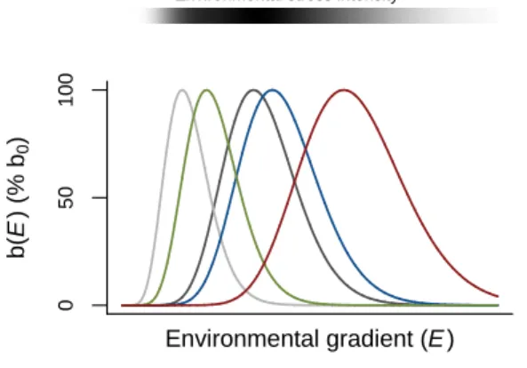
Fig. 1. Species functional responses and definition of environmental stress as assumed in the model.
554
Niches of five hypothetical species are depicted as the change in the per-capita birth rate (b) over an
555
environmental gradient (E). Note that values have been normalised to the percentage reduction in the
556
maximal per-capita birth rate, bi,0. The stress intensity of an environmental condition is calculated as
557
the average % reduction in the maximal per capita birth rate of the species. Lighter colours indicate
558
higher environmental stress intensity.
559 560 561 562 563 564 565 566 567 568 569 0 5 0 1 0 0 Environmental gradient (E ) b (E ) (% b0 )
570
Fig. 2: Upper panels: simulated changes in slopes of BEF relationships with increasing environmental
571
stress intensity (SI) for constant, increasing, decreasing, and shifts from competitive to facilitative
per-572
capita interactions under increasing environmental stress intensity. Lower panels: simulated
573
relationship between the slope of the BEF relationship under unstressed environmental conditions
574
(Slope0) and the stress intensity at which a maximal slope is attained (SImax). Red lines and dots indicate
575
unimodal relationships, blue lines and dots indicate monotonic relationships. Thick lines represent the
576
model predictions for unimodal and monotonic relationships. The grey shaded area corresponds to
577
the 95% prediction interval.
578 579 580 581 582 583 584 585 586
587
Fig. 3: Simulated changes in dominance, trait-dependent and trait-independent complementarity
588
effects with increasing environmental stress intensity (SI) for constant, increasing and decreasing
per-589
capita interactions under increasing environmental stress intensity. Red lines indicate unimodal
590
relationships, blue lines indicate monotonic relationships. Thick lines represent the mean model
591
predictions for unimodal and monotonic relationships.
592 593 594 595 596 597 598 599 600 601
602
603
604
605
Fig. 4: Left panel: Empirical observed changes in slopes of BEF relationships with increasing
606
environmental stress intensity (SI). Right panel: Empirical and modelled relationship between the slope
607
of the BEF relationship under unstressed environmental conditions (Slope0) and the stress intensity at
608
which a maximal slope is attained (SImax). Red lines and dots indicate unimodal empirical relationships,
609
blue lines and dots monotonic empirical relationships for the empirical data. The grey shaded area
610
corresponds to the 95% prediction interval for the empirical data.
611 612 613 614 615 616 617
Tables
618 619Table 1: Estimated relationship between the the slope under unstressed conditions and the stress
620
intensity at which maximal biodiversity effects are attained. Significances for model simulations are
621
expressed against the value of the empirical regression.
622
Estimate p-value Intercept empirical data 0.233 <0.001
Intercept constant interactions 0.105 <0.001
Intercept increasing interactions 0.087 <0.001
Intercept decreasing interactions 0.183 0.136
Intercept shift to facilitation 0.165 0.314
SImax empirical data -0.379 <0.001
SImax constant interactions -0.174 <0.001
SImax increasing interactions -0.163 <0.001
SImax decreasing interactions -0.305 0.38
SImax Shift to facilitation -0.311 0.68 623
624 625