Characterization of neocortical networks from high-resolution EEG: application to disorders of consciousness

(1)

HAL Id: tel-02372280

https://hal.archives-ouvertes.fr/tel-02372280

Submitted on 20 Nov 2019

HAL is a multi-disciplinary open access

archive for the deposit and dissemination of sci-entific research documents, whether they are pub-lished or not. The documents may come from teaching and research institutions in France or abroad, or from public or private research centers.

L’archive ouverte pluridisciplinaire HAL, est destinée au dépôt et à la diffusion de documents scientifiques de niveau recherche, publiés ou non, émanant des établissements d’enseignement et de recherche français ou étrangers, des laboratoires publics ou privés.

Characterization of neocortical networks from

high-resolution EEG: application to disorders of

consciousness

Jennifer Rizkallah

To cite this version:

Jennifer Rizkallah. Characterization of neocortical networks from high-resolution EEG: application to disorders of consciousness. Signal and Image processing. Université de Rennes 1 [UR1], 2019. English. �tel-02372280�

(2)

T

HESE DE DOCTORAT DE

L'UNIVERSITE

DE

RENNES

1

COMUE UNIVERSITE BRETAGNE LOIRE

ECOLE DOCTORALE N°601

Mathématiques et Sciences et Technologies de l'Information et de la Communication

Spécialité : Signal, Image et Vision

Characterization of neocortical networks from high-resolution

EEG: application to disorders of consciousness

Thèse présentée et soutenue à Rennes, le 08/11/2019

Unité de recherche : Laboratoire Traitement de Signal et de l’Image LTSI – INSERM UMR1099

Par

Jennifer RIZKALLAH

Rapporteurs avant soutenance :

Silvia Casarotto Research Fellow at the Università degli Studi di Milano Fadi Karameh Associate Professor at the American university of Beirut Composition du Jury :

Examinateurs : Catherine Marque Professeure à l’Université de Technologie de Compiègne Mohamad Khalil Professeur à l’Université Libanaise

Nicolas Farrugia Maitre de conférences à IMT Atlantique Dir. de thèse : Fabrice Wendling Directeur de recherche INSERM

Hassan Amoud Professeur à l’Université Libanaise

Co-dir. de thèse : Mahmoud Hassan Postdoctorant au LTSI, Université de Rennes 1

Invité(s)

(3)

(4)

3

ACKNOWLEDGMENTS

This work was carried out in the context of the European project LUMINOUS at Laboratoire Traitement du Signal et de l’image (LTSI), Rennes- France and at AZM center for research in biotechnology, Tripoli-Lebanon and was financed by the Institut national de la santé et de la recherche médicale (INSERM, France) and the AZM and SAADE Association (Tripoli, Lebanon).

I owe my deepest gratitude to my advisors: prof. Fabrice Wendling, prof. Hassan Amoud and Dr. Mahmoud Hassan. Without their invaluable advices, continuous support and encouragements this work would never been completed.

Besides my advisors, I would like to thank the rest of my thesis committee: prof. Silvia Casarotto, prof. Fadi Karameh, prof. Catherine Marque, prof. Mohamad Khalil, Dr. Nicolas Farrugia and prof. Naji Riachi for being a part of my thesis defense jury.

I would like to thank prof. Lotfi Senhadji for welcoming me in LTSI and the secretaries: Soizic, Patricia and Muriel for their logistical support and sympathy.

I want to thank prof. Christian Benar and prof. Jean-Louis Dillenseger for accepting to be part of my Individual Monitoring Committee (comité de suivi de thèse).

I would like to express my special thanks to Prof. Julien Modolo and Dr. Pascal Benquet for their contribution in enriching this thesis with their experiences and suggestions.

I would like to thank all the LUMINOUS project partners with whom I had the pleasure to share memorable moments and scientific collaborations during all our meetings.

Many thanks go to all the colleagues I had the opportunity to meet during these years of thesis whether in France or in Lebanon.

Finally, it is a privilege to express my sincere appreciation to all my parents, sisters and my husband for their continuous support, sacrifices and unconditional love.

(5)

(6)

5

LIST OF FIGURES

Figure 1: Brain connectivity. A) Structural connectivity refers to anatomical connections between neural elements such as fiber tracts connecting brain regions. B) Functional connectivity presents statistical dependencies between brain regions. C) Effective connectivity consists of directed causal influences one brain region produces in another. ... 32

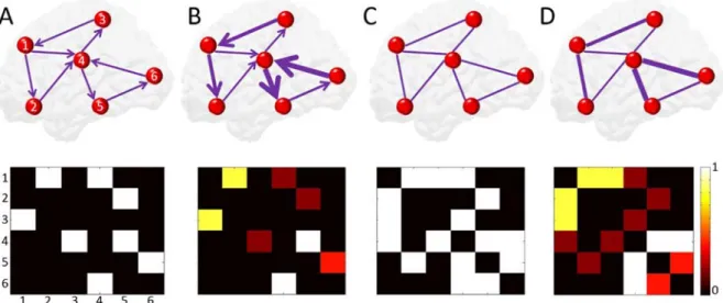
Figure 2: Graphs and adjacency matrices. A) Binary directed network. B) Weighted directed network. C) Binary undirected network. D) Weighted undirected network. ... 33

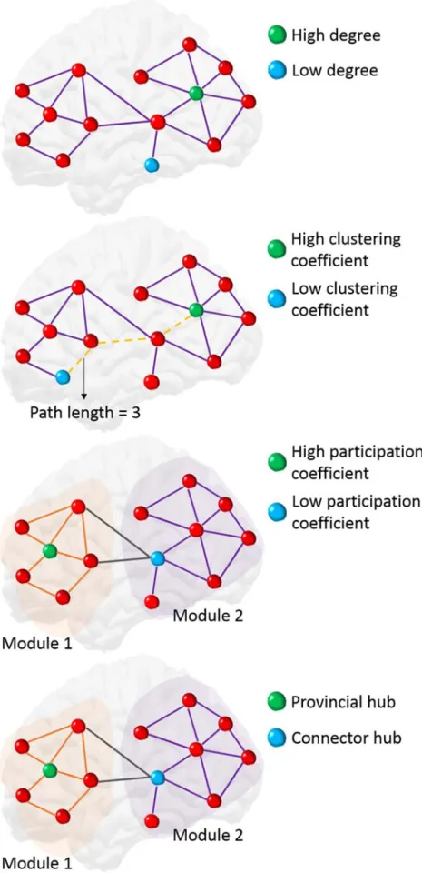
Figure 3: Illustration of some graph measures: degree, clustering coefficient, path length, modularity, participation coefficient and hubs (provincial and connector). ... 36

Figure 4: Neuroimaging techniques. A) Functional magnetic resonance imaging (fMRI). B) Magneto-encephalography (MEG). C) Electro-encephalography (EEG). ... 38

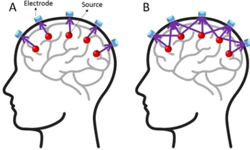
Figure 5: Volume conduction problem. A) Ideally, each electrode measures brain activity from the source below it. (b) In reality, signals recorded at each electrode are generated from several sources. ... 38

Figure 6: States of consciousness according to the level of awareness and arousal. ... 42

Figure 7: The meaningful (left) and meaningless (right) images used in the study. ... 46

Figure 8: Picture naming experimental setup. The cognitive task consisted in naming visual stimuli of two categories: meaningful and meaningless pictures. ... 47

Figure 9: CRS-R response profile (Giacino et al., 2004). ... 49

Figure 10: EEG source connectivity pipeline. EEG recorded at the scalp level are preprocessed before solving the inverse problem to obtain the regional time series. Finally, functional connectivity matrices are computed. ... 52

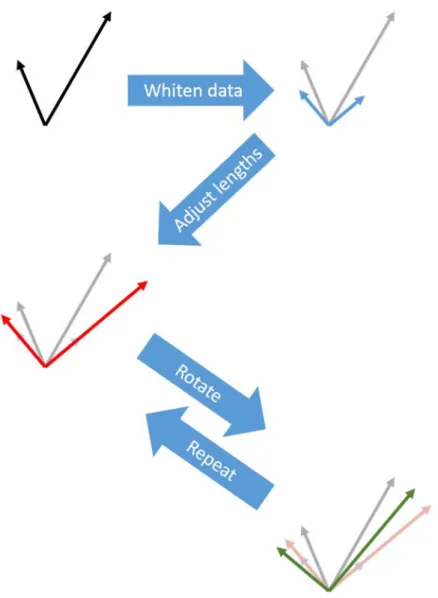
Figure 11: Symmetric orthogonalisation approach. The correlations between ROIs introduced during source reconstruction can be removed by mutually orthogonalising the ROI time-series, illustrated here for two vectors in two dimensions. An optimal set of corrected time-series is

(11)

10 reconstructed by iterating towards the closest set of orthogonal vectors to the starting time-series. The process is initialized with the closest orthonormal matrix to the uncorrected vectors, then adjusts in turn the vector magnitudes and orientations to minimize the Euclidean distance between the corrected and uncorrected time-series, adapted from (Colclough et al., 2015). .. 58

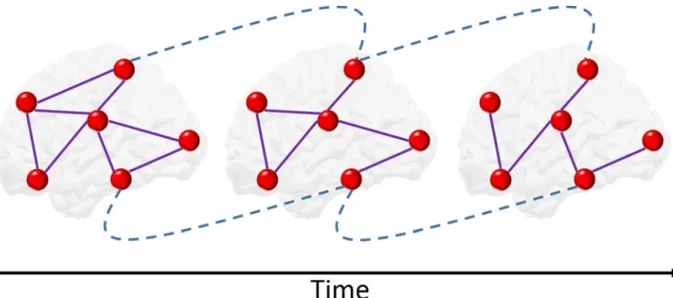
Figure 12: Multislice modularity approach. A coupling parameter that links nodes across time windows is introduced before performing the modularity maximization procedure to dynamically track modules changes during time. ... 59

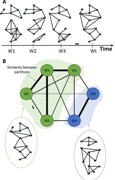
Figure 13: Modular states algorithm pipeline. (A) Computing the modules for the dynamic networks using multislice modularity method then (B) computing the similarity between the dynamic modular structures and clustering the similarity matrix into “categorical modules (adapted from by (Kabbara et al., 2019)). ... 61

(12)

11

LIST OF TABLES

Table 1: Patients demographic information: age, gender, days since injury, traumatic (T) or non-traumatic (NT) etiology and clinical best diagnosis. ... 50

(13)

(14)

13

LIST OF ABBREVIATIONS

AEC: Amplitude Envelope Correlation

AECCol: Colclough orthogonalisation approach combined with AEC

AECPas: Pascual-Marqui orthogonalisation approach combined with AEC

BEM: Boundary Element Model

BOLD: Blood Oxygen Level Dependent

Coh: Coherence

CRS: Coma Recovery Scale

CRS-R: Coma Recovery Scale Revised

DMN: Default Mode Network

DoC: Disorders of Consciousness

DSN: Dorsal Somatomotor Network

EEG: Electro-Encephalography

EMCS: Emergence from Minimally Conscious State

FC: Functional Connectivity

FDR: False Discovery Rate

FEM: Finite Element Model

fMRI: functional Magnetic Resonance Imaging

GSP: Graph Signal Processing

(15)

14 ImCoh: Imaginary Coherence

LORETA: Low resolution brain electromagnetic tomography

MCS: Minimally Conscious State

MCS+: Minimally Conscious State Plus

MCS-: Minimally Conscious State Minus

MEG: Magneto-Encephalography

MI: Mutual Information

MNE: Minimum Norm Estimate

PC: Partial Coherence

PLI: Phase Lag Index

PLV: Phase Locking Value

PLVCol: Colclough orthogonalisation approach combined with PLV

PLVPas: Pascual-Marqui orthogonalisation approach combined with PLV

ROIs: Regions Of Interests

RSNs: Resting States Networks

sLORETA: Standardized low resolution brain electromagnetic tomography

TMS: Transcranial Magnetic Stimulation

UWS: Unresponsive Wakefulness Syndrome

wMNE: weighted Minimum Norm Estimate

(16)

15

RESUME EN FRANÇAIS

Le cerveau humain est un réseau complexe et les connexions entre les régions cérébrales sont cruciales pour le traitement de l'information. Une fonction cognitive efficace est garantie lorsque le cerveau reconfigure d’une manière dynamique l'organisation de son réseau durant le temps (Bola and Sabel, 2015). Il n’est donc pas surprenant que la science des réseaux ait contribué aux domaines des neurosciences et de la neurologie au cours de la dernière décennie (Bassett and Sporns, 2017).

La neuroscience des réseaux (‘Network Neuroscience’) a été développée récemment pour mieux comprendre les systèmes neuronaux en adoptant des outils de la théorie des graphes. Ce domaine de recherche a fourni aux chercheurs une nouvelle opportunité d'évaluer, de quantifier et de caractériser les réseaux cérébraux complexes. Les études ont montré aussi que la plupart des troubles cérébraux, y compris les maladies neuro-dégénératives et mentales, sont également considérés comme des « maladies de réseau », c’est-à-dire qu’elles se caractérisent par des altérations du réseau cérébral structurel et/ou fonctionnel (Fornito et al., 2015; Stam, 2014). Du point de vue clinique, il existe donc une forte demande pour des nouvelles méthodes non invasives, basées sur les réseaux et faciles à utiliser, permettant d'identifier ces réseaux pathologiques dans la perspective de proposer de nouveaux outils de diagnostic et suivi thérapeutique.

Les techniques de neuro-imagerie peuvent être utilisées pour identifier les réseaux cérébraux impliqués dans les fonctions cérébrales normales ainsi que dans les troubles neurologiques. Dans ce contexte, l'imagerie par résonance magnétique fonctionnelle (IRMf) s'est considérablement développée au cours des trois dernières décennies et est maintenant couramment utilisée pour caractériser la connectivité cérébrale fonctionnelle (Rogers et al., 2007). Cependant, plusieurs fonctions cérébrales (normales ou pathologiques) sont très rapides et se produisent sur des périodes de temps très courtes (<1 seconde). De tels changements ne peuvent pas être suivis avec l’IRMf en raison de sa résolution temporelle intrinsèque faible (de l'ordre de 1 seconde).

L'électroencéphalographie (EEG) est une technique non invasive unique (en plus de la magnétoencéphalographie MEG), qui permet de suivre la dynamique de l’activité cérébrale à

(17)

16 la milliseconde. Des études antérieures sur les analyses de la connectivité fonctionnelle à partir de l’EEG ont été principalement réalisées au niveau des électrodes, c’est-à-dire calculer le couplage statistique entre les signaux enregistrés par les capteurs au niveau du scalp. Cependant, l'interprétation des réseaux EEG obtenus au niveau scalp (au niveau des électrodes) n'est pas simple, car les signaux sont altérés par le « volume de conduction » (Brunner et al., 2016; Van de Steen et al., 2016). La méthode appelée « connectivité de sources en EEG » est une des solutions potentielles qui réduit l’effet de ce problème et permet de suivre la dynamique des réseaux cérébraux large échelle tout en conservant l’excellente résolution temporelle de l’EEG (Hassan and Wendling, 2018; O'Neill et al., 2018).

C’est dans ce contexte que s’inscrivent mes travaux de thèse qui prolongent les développements méthodologiques et cliniques de notre équipe de recherche sur la connectivité fonctionnelle au niveau des sources cérébrales. L’objectif de mes travaux de thèse est double : i) progresser sur les aspects méthodologiques de la méthode connectivité de sources en EEG et ii) utiliser cette méthode dans une application clinique en lien avec les troubles de la conscience. Ma thèse se divise donc en deux grandes parties, avec deux études réalisées dans chaque partie. Dans la première partie (aspects méthodologiques), j’ai abordé, dans une première étude, la capacité de la méthode connectivité de sources en EEG à suivre les altérations dynamiques des réseaux cérébraux durant une tâche cognitive rapide. Puis dans une seconde étude, j’ai testé l’effet du problème de l’étalement spatial des sources sur la reconstruction des réseaux fonctionnels. Dans la deuxième partie (applications cliniques), j’ai analysé les altérations dans les réseaux cérébraux chez les patients souffrant d’un désordre de la conscience.

Aspects méthodologiques

Dans la première étude de la partie méthodologique, j’ai testé la capacité de la méthode connectivité de sources en EEG à suivre les modifications de la dynamique cérébrale durant une tâche cognitive. Nous avons choisi la tâche bien définie de dénomination d'objets visuels (DiCarlo et al., 2012), qui implique des processus cognitifs rapides (quelques centaines de ms, du début du stimulus à l’articulation) et j’ai déterminé la différence dans les réseaux fonctionnels dynamiques lors de la reconnaissance d'images significatives (‘meaningful’) et non significatives (‘meaningless’). De plus, j’ai proposé une nouvelle mesure appelée « occurrence » qui présente la probabilité que deux régions cérébrales quelconques tombent dans le même module (où les régions fortement interconnectés mais mal connectés à d'autres régions

(18)

17 sont groupées ensemble) au fil du temps, afin de suivre les changements modulaires des régions cérébrales.

Dans ce but, des données EEG haute résolution (256 électrodes) ont été collectées de 20 sujets sains. J’ai estimé les réseaux cérébraux fonctionnels en utilisant la méthode connectivité de sources en EEG. Ensuite, en utilisant des algorithmes de modularité, j’ai suivi la reconfiguration de réseaux fonctionnels lors de la reconnaissance d'images significatives (‘meaningful’) et non significatives (‘meaningless’). Les résultats ont montré une différence dans les caractéristiques des modules concernant les deux conditions en termes d’intégration (interactions entre modules) et d’occurrence (la probabilité que deux régions du cerveau soient dans le même module durant une tâche). L'intégration et l'occurrence étaient plus importantes pour les images non significatives que pour les images significatives. Ces résultats, rapportés dans un article publié dans le « Journal of neural engineering » (Rizkallah et al., 2018), ont également révélé que l'occurrence dans les régions frontales droites et occipito-temporelle gauche peuvent prédire la capacité du cerveau à reconnaître et à nommer rapidement les stimuli visuels.

Bien que la méthode connectivité de sources en EEG soit une technique prometteuse, elle reste perfectible et plusieurs problèmes méthodologiques restent ouverts (Palva and Palva, 2012; Schoffelen and Gross, 2009; Van Diessen et al., 2015) dont l’ « étalement spatial des sources » (‘spatial leakage’) qui induit des connexions parasites entre sources proches correspondant à des régions adjacentes. Pour traiter ce problème, la plupart des approches existantes reposent sur l'hypothèse que l’ « étalement spatial des sources » génère une connectivité exagérée ce qui se traduit par des corrélations à décalage de phase nul. Ainsi, ces méthodes ont résolu ce problème en supprimant les connexions à décalage nul (Nolte et al., 2004; Stam et al., 2007) ou en adoptant une approche fondée sur l'orthogonalisation (Brookes et al., 2012; Hipp et al., 2012; Pascual-Marqui et al., 2017). D’où le deuxième but de cette partie méthodologique, comparer plusieurs méthodes permettant de corriger le problème de l’étalement spatial des sources et d’autres qui ne le corrigent pas afin de déterminer l’effet de la correction de fuite sur les réseaux reconstruits.

Dans cette deuxième étude méthodologique, des signaux EEG à haute résolution (256 électrodes) ont été collectés de 30 sujets sains à l’état de repos. J’ai estimé les réseaux cérébraux en utilisant la méthode connectivité de sources en EEG en adoptant plusieurs techniques (divisées en 2 familles) pour le calcul de la connectivité. La première famille, qui ne corrige

(19)

18 pas le problème de l’étalement spatial, comprend les méthodes appelées « indice de verrouillage de phase » (‘Phase Locking Value’ PLV) et « correlation de l’amplitude de l’enveloppe » (‘Amplitude Envelope Correlation’ AEC). La deuxième famille qui le corrige en supprimant les connexions à décalage nul compris l’ « indice de décalage de phase » (‘Phase Lag Index’ PLI) et deux méthodes d’orthogonalisation combinées avec les méthodes PLV et AEC. J’ai comparé les réseaux obtenus par chaque méthode de connectivité fonctionnelle avec le réseau IRMf obtenu au repos (du Human Connectome Project -HCP-, N = 487). Les résultats montrent de faibles corrélations pour tous les réseaux EEG obtenus, cependant les réseaux PLV et AEC sont significativement corrélés avec le réseau IRMf (ρ = 0.11, p = 1.93x10-8_{et ρ = 0.06,}

p = 0.007, respectivement), alors que les autres méthodes ne le sont pas. Ces résultats, rapportés dans un article (en révision) dans « Brain Topography » (Rizkallah et al., 2019a), suggèrent que les méthodes qui corrigent le problème d’étalement spatial des sources (en supprimant les connexions à décalage nul) estiment des réseaux plus loin de ceux estimés à partir de l’IRMf.

Aspects cliniques

La deuxième partie de ma thèse s’inscrit dans le contexte du projet européen LUMINOUS (H2020 FET-Open) dont l'objectif général est d'étudier, de modéliser et de quantifier la conscience. Plusieurs études ont associé les désordres de conscience à des altérations des réseaux cérébraux fonctionnels et/ou structurels (Amico et al., 2017; Annen et al., 2018). Les désordres de conscience englobent une variété d'états de conscience, tels que l’état d’éveil sans réponse ou l’état végétatif (EV, le patient est éveillé avec seulement des mouvements réflexes (Laureys et al., 2010)), l'état de conscience minimale (ECM, le patient fait des comportements reproductibles et intentionnels (Giacino et al., 2002)) et l’émergence de l’état de conscience minimale (EECM, caractérisé par une récupération de la communication fonctionnelle et / ou de l’utilisation d’objets (Giacino et al., 2002)). Nous manquons à ce jour des méthodes fiables pour évaluer objectivement le niveau de conscience chez les patients présentant des troubles de la conscience (Laureys et al., 2004). Plusieurs techniques de neuro-imagerie ont récemment révélé des résultats importants concernant les perturbations dans les réseaux cérébraux correspondant à ces états de perte de conscience, notamment l'IRMf (Demertzi et al., 2015; Di Perri et al., 2014; Di Perri et al., 2017), la tomographie par émission de positrons (Stender et al., 2014; Thibaut et al., 2012) et EEG obtenus au niveau du scalp (Chennu et al., 2017; Sitt et al., 2014). Plusieurs patients considérés comme inconscients ont présenté des signes de suivi

(20)

19 des commandes avec des études basées sur l’IRMf (Bardin et al., 2012; Monti et al., 2010b; Owen et al., 2006) et des paradigmes actifs (Cruse et al., 2012; Goldfine et al., 2011).

Dans ce contexte, j’ai étudié l’apport de la connectivité fonctionnelle estimée à partir de l’EEG. J’ai analysé les altérations dans les réseaux cérébraux dans les désordres de conscience en utilisant la méthode connectivité de sources en EEG. Dans cette partie clinique, je me suis concentrées sur deux caractéristiques principales de réseau : l'intégration (traitement global de l'information) et la ségrégation (traitement local de l'information). Deux études ont été réalisées dans ce contexte: i) une analyse statique, dont l'objectif était de voir s'il existait un (des)équilibre entre l'intégration et la ségrégation du réseau chez les patients atteints de désordres de conscience et ii) une étude dynamique permettant de suivre les altérations dynamiques dans les réseaux cérébraux corticaux en fonction des états de conscience.

Les données EEG haute résolution ont été collectées à Liège par le « coma science group » de 82 participants à l'état de repos: 61 patients (EECM (n = 6), ECM (n = 46), et EV (n = 9)) et 21 sujets sains. J’ai estimé les réseaux cérébraux fonctionnels dans cinq bandes de fréquence différentes (delta, thêta, alpha, bêta et gamma) à l'aide de la méthode connectivité de sources en EEG. J’ai utilisé des analyses basées sur la théorie des graphes pour évaluer leur relation avec les niveaux de conscience ainsi que les différences entre les groupes de volontaires sains et les groupes de patients. Les résultats sont rapportés dans un article publié dans « Neuroimage Clinical » (Rizkallah et al., 2019b). Ils ont montré que les réseaux de patients souffrant des désordres de conscience sont caractérisés par un traitement global de l'information altéré (l'intégration des réseaux cérébraux fonctionnels diminuait avec un niveau de conscience inférieur). En outre, j’ai pu identifier deux régions cérébrales à intégration réduite impliquées entre les groupes: le précuneus gauche (impliqué dans le traitement de soi, la prise de conscience et le traitement de l'information consciente) et le cortex orbitofrontal gauche (impliqué dans la sélection d'action en fonction de contextes sensoriels et dans la perception de la douleur).

Finalement, j’ai exploré les changements dynamiques des structures modulaires du cerveau chez les patients qui ont des désordres de conscience en appliquant une nouvelle méthode développée dans l’équipe (Kabbara et al., 2019). Cette méthode consiste à évaluer la similitude entre les structures modulaires durant le temps et extraire les structures les plus représentatives de chaque group étudié. Les résultats ont montré que dans la bande gamma, les réseaux qui sont

(21)

20 les plus présents chez les sujets sains et ECM sont les réseaux cognitifs et moteurs (régions cingulate, préfrontales et centrales). Tandis que chez les sujets à l’état végétatif, j’ai trouvé le réseau visuel sensoriel. De même dans la bande beta, j’ai trouvé non seulement les réseaux cognitifs et moteurs, mais aussi le réseau responsable du langage (les régions supramarginales associées avec les régions superiortemporales et précentrales à gauche) chez les sujets sains et ECM et qui disparaissent pour les sujets EV. Enfin, dans la bande alpha, les résultats montrent que les connexions fronto-pariétales (réseau attentionnel) présentes chez les sujets sains et ECM disparaissent chez les patients EV.

(22)

21

SUMMARY IN ENGLISH

The human brain is a complex network and the connections between the brain regions are crucial for information processing. Cognitive function is guaranteed when the brain dynamically reconfigures its network organization over time (Bola and Sabel, 2015). It is then unsurprising that, in the last decade, network science has contributed to neuroscience and neurology (Bassett and Sporns, 2017).

Network Neuroscience has recently been developed to better understand neural systems by adopting graph theory tools. This area of research has provided researchers with a new opportunity to evaluate, quantify and characterize complex brain networks. Studies have also showed that most brain disorders, including neurodegenerative and mental diseases, are considered as network diseases. They are characterized by changes in the structural and/or functional brain networks (Fornito et al., 2015; Stam, 2014). Thus, from a clinical point of view, there is a strong demand for new, non-invasive, network-based and easy-to-use methods to identify these pathological networks, in order to propose new diagnostic and therapeutic monitoring tools.

Neuroimaging techniques can be used to identify brain networks involved in normal brain functions as well as in neurological disorders. In this context, functional magnetic resonance imaging (fMRI) has considerably developed during the last three decades and is now commonly used to characterize functional brain connectivity (Rogers et al., 2007). However, several brain functions (normal or pathological) are very fast and occur over very short time periods (<1 second). Such changes cannot be tracked with fMRI due to its intrinsic low temporal resolution (on the order of 1 second).

Electroencephalography (EEG) is a unique noninvasive technique (in addition to magnetoencephalography MEG), which tracks the dynamics of brain activity at millisecond time-scale. Previous studies on EEG functional connectivity have mainly been performed at the scalp level by computing the statistical coupling between the signals recorded by the sensors. However, the interpretation of the EEG networks obtained at the scalp (sensors) level is not simple, since the signals are altered by the volume conduction problem (Brunner et al., 2016; Van de Steen et al., 2016). EEG source connectivity is a potential solution which reduces the

(23)

22 effect of this problem and enables the tracking of large scale brain networks dynamics while maintaining the EEG excellent temporal resolution (Hassan and Wendling, 2018; O'Neill et al., 2018).

It is in this context that my thesis was carried out. My work here extends the methodological and clinical developments of our research team on functional connectivity at cortical level. The aim of my thesis work is twofold: i) to progress on the methodological aspects of the EEG source connectivity method and ii) to use this method in a clinical application related to the disorders of consciousness. My thesis is divided into two main parts, with two studies realized in each part. In the first part (methodological aspects), I approached, in a first study, the capacity of the EEG source connectivity method to track the brain network dynamic alterations during a fast cognitive task. Then in a second study, I tested the effect of the spatial leakage problem on the reconstructed functional brain networks. In the second part (clinical applications), I analyzed brain networks alterations in patients with disorders of consciousness, using static analysis in the first study and dynamic analysis in the second one.

Methodological aspects

In the first study of the methodological part, I tested the ability of the EEG source connectivity method to track brain dynamic changes during a cognitive task. We chose the well-defined visual object recognition and naming task (DiCarlo et al., 2012) which involves fast cognitive processes (a few hundred of ms, from stimulus onset to reaction) and I determined the differences in dynamic functional networks when recognizing meaningful and meaningless images. In addition, I proposed a new measure called "occurrence" which presents the probability of any two brain regions to fall into the same module (where highly interconnected regions and poorly connected to other regions are grouped together) over time, in order to track the brain regions’ modular changes.

For this purpose, high resolution EEG data (256 electrodes) were collected from 20 healthy subjects. I estimated the functional brain networks using the EEG source connectivity method. Then, using modularity algorithms, I followed the reconfiguration of functional brain networks during the recognition of meaningful and meaningless images. The results showed a difference in the characteristics of the modules concerning the two conditions in terms of integration (interactions between modules) and occurrence (the probability of two brain regions to be in

(24)

23 the same module during a task). Integration and occurrence values were higher for non-significant images than for meaningful images. These findings, reported in an article published in the “Journal of Neural Engineering” (Rizkallah et al., 2018), have also revealed that right frontal and left occipito-temporal regions occurrence can predict the brain's ability to recognize and to quickly name visual stimuli.

Although EEG source connectivity method is a promising technique, it remains immature and several methodological questions remain open (Palva and Palva, 2012; Schoffelen and Gross, 2009; Van Diessen et al., 2015). One of these methodological issues is the spatial leakage which induces spurious connections between adjacent brain regions. Most of the existing approaches to deal with this problem are based on the hypothesis that source leakage generates inflated connectivity manifesting as zero-phase-lag correlations. Thus, these methods solved this problem by removing zero-lag connections (Nolte et al., 2004; Stam et al., 2007) or by adopting an orthogonalisation-based approach (Brookes et al., 2012; Hipp et al., 2012; Pascual-Marqui et al., 2017). Hence, the second purpose of this methodological part is to compare several methods that correct the spatial leakage problem and others that don’t in order to test the effect of leakage correction on the reconstructed networks.

In this second methodological study, resting state high-resolution EEG signals (256 electrodes) were collected from 30 healthy subjects then I estimated brain networks using EEG source connectivity by adopting several functional connectivity techniques (divided into 2 families). The first family that does not correct the leakage problem includes the Phase Locking Value (PLV) and the Amplitude Envelope Correlation (AEC). The second family that corrects this problem by removing zero-lag correlations includes the Phase Lag Index (PLI) and two orthogonalisation methods combined with PLV and AEC techniques. I compared the networks obtained by each functional connectivity method with resting fMRI network (collected from Human Connectome Project -HCP-, N = 487). Results showed weak correlations for all the EEG networks obtained. However the PLV and AEC networks were significantly correlated with the fMRI network (ρ = 0.11, p = 1.93x10-8_{and ρ = 0.06, p = 0.007, respectively), while all}

other methods were not. These results, reported in an article (in revision) in "Brain Topography" (Rizkallah et al., 2019a), suggest that methods that correct the spatial leakage problem (by removing zero-lag correlations) estimate networks very differently from those estimated from fMRI. These results were also validated on MEG data collected in the context of the HCP.

(25)

24 Clinical aspects

The second part of my thesis is in the context of the European project LUMINOUS (H2020 FET-Open) whose general objective is to study, model and quantify consciousness. Several studies have associated disorders of consciousness with functional and/or structural brain networks alterations (Amico et al., 2017; Annen et al., 2018). Disorders of consciousness encompass a variety of consciousness states, such as the unresponsive wakefulness syndrome (UWS, the patient is awake with only reflex movements (Laureys et al., 2010)), the minimally conscious state (MCS, the patient does reproducible and purposeful behaviors (Giacino et al., 2002)) and the emergence from the minimally conscious state (EMCS, characterized by a recovered functional communication and/or object use (Giacino et al., 2002)). We lack to date reliable methods to objectively assess the level of consciousness in patients with disorders of consciousness (Laureys et al., 2004). Several neuroimaging techniques have recently revealed important results regarding brain network perturbations underlying these states of unconsciousness, notably fMRI (Demertzi et al., 2015; Di Perri et al., 2014; Di Perri et al., 2017), positron emission tomography (Stender et al., 2014; Thibaut et al., 2012) and scalp EEG (Chennu et al., 2017; Sitt et al., 2014). Several patients considered unconscious showed signs of command-following with fMRI (Bardin et al., 2012; Monti et al., 2010b; Owen et al., 2006) and EEG active paradigms (Cruse et al., 2012; Goldfine et al., 2011).

In this context, I studied the contribution of functional connectivity estimated from EEG signals. I analyzed the brain network alterations in patients with disorders of consciousness using the EEG source connectivity method. In this clinical part, I focused on two main network features: integration (global information processing) and segregation (local information processing). Two studies were performed: i) a static analysis, where the objective was to investigate if there is a balance between network integration and segregation in patients with disorders of consciousness and ii ) a dynamic study to track the dynamic alterations in cortical brain networks according to states of consciousness.

The high-resolution EEG data were collected in Liège by the “coma science group” from 82 participants at rest: 61 patients (EMCS (n = 6), MCS (n = 46), and UWS (n = 9))) and 21 healthy subjects. I estimated functional brain networks in five different frequency bands (delta, theta, alpha, beta, and gamma) using the EEG source connectivity method. I used graph theory-based analyzes to assess their relationship to the level of consciousness as well as the differences

(26)

25 between groups of healthy volunteers and patients. These results are reported in an article published in "Neuroimage Clincal" (Rizkallah et al., 2019b). They showed that networks of patients with disorders of consciousness were characterized by impaired global information processing (the functional brain networks integration decreased with lower level of consciousness). Moreover, I was able to identify two common anatomical brain regions with decreased integration that were involved between groups: the left precuneus (engaged in self-related processing, awareness and conscious information processing) and the left orbitofrontal cortex (engaged in action selection depending on emotional and sensory contexts and in pain perception).

Finally, I applied a new method developed very recently by our team (Kabbara et al., 2019) to explore the brain modular states dynamic changes in healthy subjects and patients with disorders of consciousness. This method consists of assessing the similarity between the modular states over time and extracting the most representative states for each group. Results in the gamma band were mostly seen in the cognitive and motor networks (cingulate, prefrontal and central regions) in healthy subjects and MCS patients, whereas in UWS patients, they were found mostly in the sensory visual network. As for the beta band, they were not only located in the cognitive and motor networks, but also in the language network (the supramarginal regions associated with the super-temporal and pre-central regions on the left) in healthy subjects and MCS, but not in the UWS patients. Finally, in the alpha band, states were found in the fronto-parietal regions (attentional network) in healthy subjects and MCS patients but not in UWS patients.

(27)

(28)

27

CHAPTER 1: GENERAL

INTRODUCTION

The human brain is a network by nature: connections between neurons are crucial for information processing. An efficient cognitive function is guaranteed when the brain dynamically reconfigures its network organization at multiple time scales (Bola and Sabel, 2015; Braun et al., 2015). It is therefore unsurprising that network science has contributed to the fields of neuroscience and neurology in the last decade (Bassett and Sporns, 2017). A relatively new research field, referred to as network neuroscience has provided researchers with an extraordinary opportunity to assess, quantify and understand the multifaceted features of complex brain networks, using graph theoretical analysis. On the other hand, emergent evidence shows that most brain disorders, including neurodegenerative diseases and mental illnesses, are also currently considered as network diseases, i.e. they are characterized by alterations in the structural/functional brain network (Fornito et al., 2015; Stam, 2014). Thus, the demand is high for non-invasive, network-based and easy-to-use methods to identify these pathological networks in the perspective of proposing new diagnostic and therapeutic follow-up tools.

Neuroimaging techniques can be used to identify brain networks involved in normal brain functions (picture naming, learning, etc.) as well as in neurological disorders. In this context, functional Magnetic Resonance Imaging (fMRI) has considerably developed during the past three decades and is now commonly used to characterize brain connectivity (Rogers et al., 2007). However, several brain functions (normal or pathological) are very fast and occur over very short time periods (< 1second). Such changes cannot be tracked with fMRI due to intrinsic low time resolution (in the order of 1 s).

Magneto/ Electro-encephalography (M/EEG) are unique non-invasive techniques which enable the tracking of brain dynamics on a millisecond time-scale. Most previous studies on M/EEG functional connectivity analyses were mainly performed at the sensor level, i.e. computing correlation between recorded signals from the sensors.

(29)

28 However, the interpretation of M/EEG networks obtained at the scalp level is not straightforward, since scalp/sensor M/EEG signals are corrupted by the volume conduction due to the head electrical conduction properties (Brunner et al., 2016; Van de Steen et al., 2016). EEG source-space connectivity is a potential solution which reduces the aforementioned volume conduction and enables the tracking of large-scale brain network dynamics on a sub-second time-scale (Hassan and Wendling, 2018; O'Neill et al., 2018). In our first study, we tested the ability of this method to track brain dynamic changes during a cognitive task. We chose the well-defined visual object recognition and naming task (DiCarlo et al., 2012) which involves fast cognitive processes (a few hundred ms from stimulus onset to reaction). Moreover, we proposed a new graph measure called ‘occurrence’ which consists of measuring the probability of any two nodes to fall in the same module over time, to track the brain regions’ modular changes during time.

Although EEG source connectivity is a promising technique, it is still immature and methodological aspects should be carefully accounted for to avoid pitfalls (Palva and Palva, 2012; Schoffelen and Gross, 2009; Van Diessen et al., 2015). One of these methodological considerations is the spatial leakage problem (i.e. presence of spurious connections between adjacent regions). To deal with this problem, most existing approaches are based on the hypothesis that leakage generates inflated connectivity between estimated sources, which manifests as zero-phase-lag correlations. Thus, these methods dealt with the leakage problem by removing the zero lag connections (Nolte et al., 2004; Stam et al., 2007) or adopting orthogonalisation-based approach (Brookes et al., 2012; Hipp et al., 2012; Pascual-Marqui et al., 2017). In our second analysis, we presented a comparative study to test the effect of leakage correction on the reconstructed networks by comparing methods that correct the source leakage problem and those that do not.

On the other hand, emerging evidence associates disorders of consciousness (DoC) with alterations in functional and/or structural brain networks (Amico et al., 2017; Annen et al., 2018). DoC encompass a variety of consciousness states, such as the unresponsive wakefulness syndrome (UWS; wakefulness with only reflex movements) (Laureys et al., 2010; Monti et al., 2010a), the minimally conscious state (MCS; reproducible and purposeful behavior) (Giacino et al., 2002), and emergence from the minimally conscious state (EMCS; characterized by recovered functional communication and/or object use) (Giacino et al., 2002). To date, we lack

(30)

29 reliable methods to objectively assess consciousness level in patients with disorders of consciousness (Laureys et al., 2004).

Significant discoveries regarding the neural correlates underlying these states of unconsciousness have recently been made by several neuroimaging techniques including functional MRI (fMRI) (Demertzi et al., 2015; Di Perri et al., 2014; Di Perri et al., 2017), positron emission tomography (PET) (Stender et al., 2014; Thibaut et al., 2012) and scalp EEG (Chennu et al., 2014; Chennu et al., 2017; Sitt et al., 2014). Several patients considered unconscious showed signs of command-following with fMRI (Bardin et al., 2012; Monti et al., 2010b; Owen et al., 2006) and EEG active paradigms (Cruse et al., 2012; Goldfine et al., 2011). In our study, we tackled the brain alterations in DOC using EEG source connectivity and focused on two network characteristics: integration (global information processing) and segregation (local information processing). Two studies were performed: i) A static analysis, where the objective was to investigate if a balance between network integration and segregation in DOC patients exists and to identify the involved brain regions that differentiate between different groups and ii) a dynamic study to track time-varying alterations in cortical brain networks as a function of clinical consciousness levels.

This thesis was part of the Future Emerging Technologies (H2020-FETOPEN-2014-2015-RIA under agreement No. 686764, “LUMINOUS”) as part of the European Union’s Horizon 2020 research and training program 2014–2018 (http://www.luminous-project.eu/). The general objective of the LUMINOUS project is to study, model, quantify, and alter observable aspects of consciousness. The conceptual framework of the project rests on information theoretic developments that link consciousness to the amount of information that a physical system can represent and generate as an integrated whole, and from the related idea that consciousness can be quantified by metrics reflecting information processing and representation complexity. This thesis was also financed by the AZM and SAADE Association, Tripoli, Lebanon.

This manuscript is organized as follows: In chapter 2, we report the background of the brain networks and disorders of consciousness and we state the problems we aim to tackle. In chapter 3, we describe all the materials and methods. Results are presented in chapter 4, under the form of published or under revision articles. For each article, a synthesis presenting the objectives, methods and results are provided. Finally, conclusions and perspectives are given in chapter 5.

(31)

(32)

31

CHAPTER 2. BACKGROUND AND

PROBLEM STATEMENT

In this chapter, we describe the basic notions of the methods and approaches used during the thesis such as brain connectivity, graph theoretical approaches and network measures, in addition to some neuroimaging techniques and the EEG source connectivity method. From the application viewpoint, we introduce the basic notions and the clinical need of the brain disorders of consciousness. Finally, the general and specific objectives of this thesis will be described.

2.1. Brain connectivity and graphs

At the macroscopic scale, emerging evidence shows that brain functions arise from continuous communications between spatially distant brain regions, called brain connectivity (Bullmore and Sporns, 2009). Three main types of brain connectivity can be distinguished: structural, functional and effective connectivity (Bullmore and Sporns, 2009; Rubinov and Sporns, 2010).

The structural connectivity (Fig1.A), also known as anatomical connectivity, refers to a pattern of anatomical connections summarizing synaptic links between neurons at the micro scale or projections between brain regions (measured using diffusion imaging) at the macro scale. This physical organized connection pattern is symmetric and stable at short time range (seconds to minutes) and is subjected to significant morphological change at longer time scales (hours and days) (Dennis et al., 2013). A number of studies examined the structural brain networks at rest (Hagmann et al., 2008; Li et al., 2013; Van Den Heuvel and Sporns, 2011). Moreover, it has been shown that structural connectivity analysis is sensitive and detects alterations of brain networks in neurological diseases (Fornito et al., 2015; Liu et al., 2014; Mallio et al., 2015) and during development or learning (Hagmann et al., 2010; Scholz et al., 2009).

Functional connectivity (FC) (Fig1.B) describes patterns of dynamic interactions, usually computed from time series data (recorded from functional neuroimaging techniques such as electro-encephalography (EEG), magneto-encephalography (MEG) or functional magnetic

(33)

32 resonance imaging (fMRI)) and estimates their statistical couplings. Unlike structural connectivity, FC may change over the sub-second scale. It can be estimated by calculating, for instance, the correlation, spectral coherence, phase-locking value or amplitude envelope correlation of all elements of the brain, regardless if they are directly connected or not (Goñi et al., 2014). In this thesis, we are interested in this type of brain connectivity (several FC methods will be fully described in section 3.2.2). The FC was widely used to study brain information processing at rest (Allen et al., 2014; Baker et al., 2014; Brookes et al., 2014; Kabbara et al., 2017; Yuan et al., 2012), during task (Bassett et al., 2011; Hassan et al., 2015; O’neill et al., 2017) and to detect network disruptions in brain disorders (Chennu et al., 2017; Engels et al., 2017; Hassan et al., 2016; Hassan et al., 2017; Kabbara et al., 2018).

Effective connectivity consists of directed causal influences one brain region produces in another. It can be measured using methods such as Granger causality (Granger, 1969), transfer entropy or methods based on autoregressive models (Friston et al., 2003). Then, it is, like functional connectivity, time varying and can change rapidly (sub-second time scale).

Figure 1: Brain connectivity. A) Structural connectivity refers to anatomical connections between neural elements such as fiber tracts connecting brain regions. B) Functional connectivity presents statistical dependencies between brain regions. C) Effective connectivity consists of directed causal influences one brain region produces in another.

Mapping of brain connectivity is rapidly increasing (Fornito et al., 2016). It consists of presenting the network as graph (Bullmore and Sporns, 2009). Such mapping typically starts by identifying a set of nodes (or vertices), and then attempts to estimate the set of edges (or links) between these nodes. Depending on the nature of edges, graphs can be classified into four types: directed/undirected and weighted/binary graphs (Sporns, 2011). Graph can also be represented by connectivity matrices known as “adjacency matrices”, where nodes are represented by rows or columns, and edges are represented by matrix elements (Fig2). In directed graphs, an edge between two nodes represents the connection from a specific node to the other and the corresponding adjacency matrices are not symmetrical (Fig2.A and B).

(34)

33 However, in undirected graphs, edges do not have any direction and the connectivity matrices are symmetric (Fiedler, 1973) (Fig2.C and D). Binary or un-weighted graphs are obtained by applying a threshold on the adjacency matrices of the weighted graphs. In weighted networks, matrix elements are continuous values often normalized between 0 and 1. In contrast, in binary matrices, elements are either 0 (no connection) or 1 (connection exists).

Figure 2: Graphs and adjacency matrices. A) Binary directed network. B) Weighted directed network. C) Binary undirected network. D) Weighted undirected network.

2.2. Graph measures

Once the brain network is modeled by a graph, several metrics can be extracted to describe the network properties at different levels (Rubinov and Sporns, 2010). Here we describe some of the most relevant measures in the context of brain network analysis. Some graph measures are illustrated in Fig3.

2.2.1. Segregation (local)

 Clustering coefficient:

Clustering coefficient is one of the main measures used to quantify network segregation. It is defined as the number of existing connections between the neighbors’ node divided by all the possible connections between them (Watts and Strogatz, 1998)

(35)

34

 Modularity

The modularity consists of partitioning a network into a number of clusters or modules, also called communities, where nodes in the same module are highly interconnected but poorly connected to other groups of nodes (Sporns and Betzel, 2016). Each module can act in parallel and nearly independently to achieve its goals, and the success or failure of each module does not affect other modules (Fornito et al., 2016). The intra-module degree is one of the features that can be extracted from modules to quantify network segregation.

2.2.2. Integration (global)

 Path length:

A path length describes how close on average a node is connected to all the other ones. In a binary network, the path length between two nodes is the number of connecting edges. In a weighted network, the length of a path represents the sum of the edge weights (Sporns, 2011).

 Global efficiency:

Global efficiency is the average inverse shortest path length (Latora and Marchiori, 2001). It describes how efficiently the network shares information. A network with high global efficiency indicates that, on average, nodes are reached by short communications.

 Participation coefficient

The participation coefficient measures the diversity of a node inter-modular connections (Guimera and Amaral, 2005). Nodes with high participation coefficients interconnect multiple modules together.

2.2.3. Hubness

 Degree and strength:

The degree is the number of connections of a node. The strength is another measure similar to the degree, but it considers the node weights and uses them in the weighted graphs. These measures provide information about how highly and strongly connected is the node. Generally, highly connected nodes are very influential on their neighbors (Bullmore and Sporns, 2009).

(36)

35

 Betweenness centrality:

The betweenness centrality is the percentage of short paths that include the node (the shortest path length is the minimum distance or steps between two nodes) (Freeman, 1977). High betweenness centrality nodes have a large influence on the information flow through the network. It is also used to find hub nodes in a network.

 Hubs:

Hubs are nodes that connect communities, usually with a high degree, short average path length and high centrality. They play a key role in establishing and maintaining an efficient communication in a network. In addition, hubs can be classified into provincial (mostly connected to nodes within their own module) and connector hubs (connected to several different modules) (van den Heuvel and Sporns, 2013).

(37)

36

Figure 3: Illustration of some graph measures: degree, clustering coefficient, path length, modularity, participation coefficient and hubs (provincial and connector).

(38)

37

2.3. Neuroimaging techniques

Neuroimaging techniques are used to map the brain activity. They are divided into two parts: structural and functional. As we are interested in the functional brain connectivity, we describe in these sub-sections the three main techniques used to map the functional brain activity at large scale.

2.3.1. Functional magnetic resonance imaging (fMRI)

fMRI (Fig4.A) is a non-invasive technique used to record brain activity by measuring the in vivo blood flow changes (Huettel et al., 2004). It measures the “blood oxygen level dependent” (BOLD) signals, a non-direct measure of the neural activity. Its concept is based on the fact that increased activity in a particular part of the brain increases oxygenated blood flow. This technique provides excellent spatial resolution (about 1-3 mm) but it is limited in temporal resolution since the BOLD response inferred from the hemodynamic changes takes time (1-2 s) (Logothetis et al., 2001). Thus low temporal resolution (about 1second) is not sufficient to tracking the dynamics of brain networks at sub-second time scale, one of the main objectives of my thesis.

2.3.2. Magneto-encephalography (MEG)

The MEG (Fig4.B) detects the magnetic fields associated with the intracellular current flow within neurons. An important advantage of MEG is that magnetic fields are not attenuated or distorted when recorded from the sensor level (Gallen et al., 1995). Moreover, this technique has an excellent time resolution (below 1 ms). On the other hand, MEG involves greater practical difficulties, as it is expensive and its use for long time periods is very complicated as is the case in DoC patients for example.

2.3.3. Electroencephalography (EEG)

EEG (Fig4.C) records the fluctuations of the electric fields generated when neurons communicate, using electrodes placed on the scalp (Buzsaki et al., 2012). EEG consists of a wave that varies in time; it contains frequency components that can be analyzed separately. The main frequencies (rhythms) of the human EEG waves are delta (0.5 - 4.5 Hz), theta (5 - 8 Hz), alpha (8 – 13 Hz), beta (13 – 30 Hz) and gamma (30 – 45 Hz). The main advantage of the EEG technique are the excellent time resolution (in order of milliseconds), the non-invasiveness and

(39)

38 the ease-of-use at the patient’s bedside, which makes it very practical for patients with impaired consciousness for instance (Chennu et al., 2014; Chennu et al., 2017; Harrison and Connolly, 2013). In this thesis, we used dense-EEG (256 electrodes).

Figure 4: Neuroimaging techniques. A) Functional magnetic resonance imaging (fMRI). B) Magneto-encephalography (MEG). C) Electro-Magneto-encephalography (EEG).

2.4. EEG source connectivity

Until the last decades, most EEG FC studies were performed at the sensor level by computing the statistical couplings between recorded signals. However, the biological interpretation of corresponding network alterations is not straightforward, since scalp EEG signals can be severely corrupted by the “volume conduction” due to the head electrical conduction properties and the “field spread” since single brain source activity can be collected by multiple sensors (Brunner et al., 2016; Van de Steen et al., 2016; Van Diessen et al., 2015), see Fig5. Several studies have indeed reported the limitations of computing connectivity at the EEG scalp level (see for review (Hassan and Wendling, 2018; Schoffelen and Gross, 2009). Moreover, scalp analysis does not allow making inferences about interacting brain regions.

Figure 5: Volume conduction problem. A) Ideally, each electrode measures brain activity from the source below it. (b) In reality, signals recorded at each electrode are generated from several sources.

(40)

39 A potential solution is the emerging technique called “EEG source connectivity” (De Pasquale et al., 2010; Hipp et al., 2012; Mehrkanoon et al., 2014), which is supposed to reduce the aforementioned problems by directly identifying the brain networks at the cortical level with a high time/space resolution (Hassan and Wendling, 2018). This method involves two main steps: i) solve the ill-posed EEG inverse problem to reconstruct the dynamics of brain sources and ii) compute the statistical couplings between the reconstructed sources, which will be described in the next chapter.

2.5. Thesis objectives

2.5.1. Methodological development

The main advantages of the EEG source connectivity method is the possibility to provide high time /space resolution brain networks. On one hand, this method was used to track dynamics of brain networks during sub-second tasks such as press button task (O’neill et al., 2017), motor imagination task of right-hand flexion for instance (Edelman et al., 2015), and finger movements cued by visual stimuli (Babiloni et al., 2005). To what extent this method can differentiate between two conditions (meaningful vs. meaningless pictures) is less explored. Here, we chose the visual object recognition and naming task (DiCarlo et al., 2012) to test the ability of this method to track the brain dynamics (to assess how functional brain network modules dynamically reconfigure) during the recognition of two object categories (meaningful and meaningless pictures). Moreover, we used this technique to see if there is a correlation between network modularity and the reaction time of the participants when meaningful pictures are presented. During this study, we introduced a new parameter called ‘the occurrence’ which present the probability of any two nodes to fall in the same module over time. Study details and results will be reported in chapter 4 – study 1.

On the other hand, as this method involves several steps from de-noising the scalp signals to reconstructing the source signals, several methodological aspects should be carefully accounted for to avoid pitfalls. Some of these parameters were analyzed, such as the head model (Liu et al., 2018) and EEG reference choice (Hu et al., 2018; Liu et al., 2015). “Source leakage” or “spatial leakage” is also one of the issue facing the source connectivity method (Hipp et al., 2012) since the functional connectivity at the source level reduces the effect of the field spread but it does not totally suppress its effects (Brookes et al., 2012). Spurious connections can be

(41)

40 created between the estimated time-series of adjacent regions. This effect is called “source leakage” or “spatial leakage”.

To deal with the aforementioned “source leakage” problem, few approaches have been proposed and they are centered on removing the edges between the very close sources (De Pasquale et al., 2010; de Pasquale et al., 2012). More recently, a number of methods were developed to remove zero-lag correlation based on the hypothesis that leakage generates inflated connectivity between estimated sources, which manifests as zero-phase-lag correlations (Brookes et al., 2012; Drakesmith et al., 2015). Un-mixing methods, called ‘leakage correction’, have been reported to force the reconstructed signals to have zero cross-correlation at lag zero. Some of the methods remove zero-lag connections when extracting FC measures as phase lag index (PLI) (Stam et al., 2007) or the imaginary coherence (ImCoh) (Nolte et al., 2004). Others remove the zero-lag connections before performing any connectivity analysis by adopting orthogonalisation-based approach (Brookes et al., 2012; Colclough et al., 2015; Hipp et al., 2012; Pascual-Marqui et al., 2017). However, several studies described the presence of these connections and proved their importance since not all zero-lag connections are spurious (Gollo et al., 2014; Roelfsema et al., 1997). Accordingly, by removing these connections, true near zero-lag connections can still be undetected (Finger et al., 2016; Palva et al., 2018; Pascual-Marqui et al., 2017; Wang et al., 2018).

Here, our objective is to study the effect of removing zero-lag connections on the reconstructed networks. Two families of FC methods were tested on rest EEG data: i) the FC metrics that do not remove the zero-lag-phase connectivity including the phase locking value (PLV) and the amplitude envelope correlation (AEC) and ii) the FC metrics that remove the zero-lag connections such as the phase lag index (PLI) and two orthogonalisation approaches combined with PLV (PLVCol – PLV combined with the symmetric orthogonalisation technique

(Colclough et al., 2015) and PLVPas – PLV combined with the innovations orthogonalisation

technique (Pascual-Marqui et al., 2017)) and AEC (AECCol – AEC combined with the

symmetric orthogonalisation technique (Colclough et al., 2015) and AECPas –AEC combined

with the innovations orthogonalisation technique (Pascual-Marqui et al., 2017)). FC matrices obtained were compared to fMRI connectivity matrices (used as a ground truth) in order to determine which connectivity network is the most similar and correlated to fMRI networks. Study details and results will be reported in chapter 4 – study 2.

(42)

41

2.5.2. Clinical application

An emerging evidence in network neuroscience proved that neurological disorders are related to alterations in the structural and functional brain connectivity (Fornito and Bullmore, 2015; Fornito et al., 2015; Stam, 2014). Many studies were performed to compare between brain networks of healthy subjects and those of patients with brain disorders in order to identify alterations in networks associated with transition from normal to pathological state (Fornito et al., 2016; Monti et al., 2010b; Tijms et al., 2013).

Network neuroscience has revealed valuable information about the functional networks involved in epilepsy (Jmail et al., 2016; Nissen et al., 2017), Alzheimer (Engels et al., 2017; Stam et al., 2006), schizophrenia (Alexander-Bloch et al., 2010; Bassett et al., 2008; Damaraju et al., 2014), depression (Lu et al., 2013; Zhang et al., 2011) and Parkinson disease (Baggio et al., 2015; Hata et al., 2016). The identification of the altered brain regions related to neurological diseases allowed better understanding of the neural mechanisms underlying brain disorders, and consequently better patients monitoring.

One of these neurological pathologies is the disorders of consciousness (DOC). Severe brain injury can rob us of consciousness, whenever temporarily or forever. This can be caused by trauma to the head or by non-traumatic causes, such as hemorrhage or ischemia (Bagnato et al., 2010). Patients surviving brain injury typically go through a sequence of progressive stages towards recovery (Giacino et al., 2014). These patients are mainly characterized by dissociation between awareness and arousal (Bernat, 2009; Laureys, 2005).

Patients in coma show no signs of arousal or awareness. They typically only exhibit reflex activities and do not respond to external stimuli, even strong and obnoxious ones (Laureys et al., 2015). Patients who recovered from coma, but entered a vegetative state, have wake and sleep cycles but show no signs of awareness of the external world (remain unresponsive to any external stimulation). This state is known as the unresponsive wakefulness syndrome (UWS) (Laureys et al., 2010; Monti et al., 2010a). If the vegetative state persists for more than one month, the percentage of recovery becomes very low (only around 20% of UWS patients will regain responsiveness within two years (Estraneo et al., 2013)). When patients show minimal, non-reflexive, yet reproducible behavioral signs of consciousness, they are considered to be in the minimally conscious state (MCS) (Giacino et al., 2002). This group is subcategorized into

(43)

42 MCS- and MCS+ based on the level of complexity of the observed behavioral responses. MCS+ patients show the ability to understand language and follow simple commands (Bruno et al., 2011; Bruno et al., 2012). Once patients restore reliable communication and/or functional object use, they are considered to emerge from MCS (EMCS) (Giacino et al., 2014; Laureys et al., 2004). States of consciousness according to the level of awareness and arousal are presented in Fig6.

Figure 6: States of consciousness according to the level of awareness and arousal.

Establishing a proper clinical diagnosis in disorders of consciousness is not straightforward (Gantner et al., 2013). Behavioral clinical assessment methods like the Glasgow Coma Scale (Jones, 1979), the Coma Recovery Scale (CRS) (Giacino et al., 1991), or the Coma Recovery Scale Revised (CRS-R) (Giacino et al., 2004) are based on the observation of motor and oro-motor behaviors at the bedside and measure patients behavioral responsiveness.

However, absence of responsiveness does not necessarily correspond to absence of awareness (Giacino et al., 2014; Sanders et al., 2012). Some patients might have consciousness but not accessible through R (Gosseries et al., 2014; Schiff and Fins, 2016). Using only the CRS-R has led to high rates of misdiagnosis of the true level of consciousness in these patients (more than 40% of UWS patients have reportedly been misdiagnosed) (Schnakers et al., 2009). A range of motor-independent neuroimaging technologies have been developed to avoid

(44)

43 diagnostic error intrinsic to behavioral assessment and help the clinical differentiation between different groups (Bruno et al., 2010; Di Perri et al., 2016; Sanders et al., 2012).

Emerging evidence associates DoC with alterations in functional and/or structural brain networks, mainly those sustaining arousal and awareness (Amico et al., 2017; Annen et al., 2016; Annen et al., 2018; Bodien et al., 2017; Boly et al., 2012; Fernández‐Espejo et al., 2012; Koch et al., 2016; Owen et al., 2009). Previous EEG network-based studies, in the context of DOC, have been performed at the scalp level (Chennu et al., 2014; Chennu et al., 2017; Estraneo et al., 2016) with satisfactory accuracies in classifying UWS and MCS patients (Chennu et al., 2017; Engemann et al., 2018; Sitt et al., 2014).

Since conscious processing involves synchronization of locally generated oscillations between remote groups of neurons (Melloni et al., 2007), high-density EEG functional connectivity at the source level is a promising approach to track such synchronizations. Our objectives was to i) explore the changes in the network topology (integration and segregation) as a function of clinical consciousness levels and ii) track dynamic functional networks alterations in the case of DoC patients. To do so, we combined EEG source connectivity with graph theory, applied to resting-state high-density-EEG (256 channels) data recorded from DoC patients, whose diagnosis has been established based on the Coma Recovery Scale-Revised (CRS-R). Two studies have been conducted in this context (static and dynamic). Studies details and results will be reported in chapter 4 – study 3 and study 4.

(45)

(46)

45

CHAPTER 3. MATERIALS

AND METHODS

In this chapter we present the materials and methods used in this thesis. First, we present the three databases used to achieve the objectives of this thesis: i) track the dynamic brain network modularity changes during the recognition of meaningful and meaningless visual images ii) study the effect of removing zero-lag connections on networks reconstruction and the effect of EEG montages and iii) track functional networks alterations in the case of DoC patients and identify brain regions involved between groups in a static and dynamic way. Second, we describe the methods used to solve the inverse problem and to obtain the functional connectivity matrices. Third, we present the concept of dynamic connectivity and the modularity analysis.

3.1. Database

3.1.1. Study 1: BrainGraph database (picture naming)

Dense-EEG signals (256 channels, EGI, Electrical Geodesic Inc.) were recorded from twenty right-handed healthy participants (ten women and ten men; mean age 23 y). Experiments were performed in accordance with the relevant guidelines and regulations of the National Ethics Committee for the Protection of Persons (CPP), (BrainGraph study, agreement number 2014-A01461-46, promoter: Rennes University Hospital), which approved all the experimental protocol and procedures. All participants in the study provided written informed consents.

80 meaningful and 40 meaningless pictures (presented in Fig8), taken from the Alario and Ferrand database (Alario and Ferrand, 1999), were displayed on a screen as black drawings on a white background using E-Prime 2.0 software (Psychology Software Tools, Pittsburgh, PA). Subjects were asked to name the meaningful images. They were informed about the presence of meaningless pictures in the experiment and were instructed to say nothing when viewing them. The same number of stimuli was used in the further analysis by selecting 40 meaningful images (the same for all subjects).

(47)

46