RESEARCH OUTPUTS / RÉSULTATS DE RECHERCHE
Author(s) - Auteur(s) :
Publication date - Date de publication :
Permanent link - Permalien :
Rights / License - Licence de droit d’auteur :
Bibliothèque Universitaire Moretus Plantin
Institutional Repository - Research Portal
Dépôt Institutionnel - Portail de la Recherche
researchportal.unamur.be
University of Namur
Featured Model-based Mutation Analysis
Devroey, Xavier; Perrouin, Gilles; Papadakis, Mike; Legay, Axel; Schobbens, Pierre;
Heymans, Patrick
Published in:
Proceedings of the 38th international conference on Software Engineering
DOI:
10.1145/2884781.2884821
Publication date:
2016
Document Version
Peer reviewed version
Link to publication
Citation for pulished version (HARVARD):
Devroey, X, Perrouin, G, Papadakis, M, Legay, A, Schobbens, P & Heymans, P 2016, Featured Model-based
Mutation Analysis. in Proceedings of the 38th international conference on Software Engineering. ICSE '16, ACM
Press, Austin, TX, USA, pp. 655-666. https://doi.org/10.1145/2884781.2884821
General rights
Copyright and moral rights for the publications made accessible in the public portal are retained by the authors and/or other copyright owners and it is a condition of accessing publications that users recognise and abide by the legal requirements associated with these rights. • Users may download and print one copy of any publication from the public portal for the purpose of private study or research. • You may not further distribute the material or use it for any profit-making activity or commercial gain
• You may freely distribute the URL identifying the publication in the public portal ?
Take down policy
If you believe that this document breaches copyright please contact us providing details, and we will remove access to the work immediately and investigate your claim.
Featured Model-based Mutation Analysis
Xavier Devroey
PReCISE Research Center University of Namur, Belgium
Gilles Perrouin
∗PReCISE Research Center University of Namur, Belgium
Mike Papadakis
SnT, SERVAL Team University of Luxembourg [email protected]Axel Legay
INRIA Rennes, France
Pierre-Yves Schobbens
PReCISE Research Center, University of Namur, Belgium [email protected]
Patrick Heymans
PReCISE Research Center, University of Namur, Belgium
ABSTRACT
Model-based mutation analysis is a powerful but expensive testing technique. We tackle its high computation cost by proposing an optimization technique that drastically speeds up the mutant execution process. Central to this approach is the Featured Mutant Model, a modelling framework for mutation analysis inspired by the software product line par-adigm. It uses behavioural variability models, viz., Featured Transition Systems, which enable the optimized generation, configuration and execution of mutants. We provide results, based on models with thousands of transitions, suggesting that our technique is fast and scalable. We found that it outperforms previous approaches by several orders of mag-nitude and that it makes higher-order mutation practically applicable.
Keywords
Mutation Analysis, Variability, Featured Transition Systems
CCS Concepts
•Software and its engineering → Software testing and debugging; Software product lines; •General and reference → Performance;
1.
INTRODUCTION
Mutation analysis is an established technique for either evaluating test suites’ effectiveness [5, 24, 50] or supporting test generation [23, 50, 54]. It works by injecting artificial defects, called mutations, into the code or the model under test, yielding mutants, and measures test effectiveness based on the number of detected mutants.
Researchers have provided evidence that detecting mu-tants results in finding real faults [5, 33] and that tests de-signed to detect mutants reveal more faults than other
test-∗
FNRS Postdoctoral Researcher
Permission to make digital or hard copies of all or part of this work for personal or classroom use is granted without fee provided that copies are not made or distributed for profit or commercial advantage and that copies bear this notice and the full cita-tion on the first page. Copyrights for components of this work owned by others than ACM must be honored. Abstracting with credit is permitted. To copy otherwise, or re-publish, to post on servers or to redistribute to lists, requires prior specific permission and/or a fee. Request permissions from [email protected].
ICSE ’16, May 14-22, 2016, Austin, TX, USA
c
2016 ACM. ISBN 978-1-4503-3900-1/16/05. . . $15.00 DOI:http://dx.doi.org/10.1145/2884781.2884821
ing criteria [7, 50]. This has been shown to be the case for model-based mutation too: Aichernig et al. [1] report that model mutants lead to tests that are able to reveal imple-mentation faults that were neither found by manual tests, nor by the actual operation, of an industrial system. In ad-dition, model-based mutation’s premise is to identify defects related to missing functionality and misinterpreted specifi-cations [13]. This is desirable since code-based testing fails to identify these kinds of defects [28, 62].
Despite its power, mutation analysis is expensive, due to the large number of mutants that need to be generated and assessed with the candidate test cases. While this problem has been researched for code-based mutation, e.g., [32,55], it remains open in the model-based context. Since typical real-word models involve thousands of mutants and test suites involve thousands of test cases, millions of test executions are needed. Addressing this problem is therefore vital for the scalability of mutation. This a known issue that requires further research, as pointed out in the surveys of Jia and Harman [31], and Offutt [50].
To address this problem, we take inspiration from past research on software product lines (SPL). As suggested in our vision paper [18], we propose an approach to model mu-tants as members (also called variants or products) of an SPL. Considering mutants as part of a family rather than in isolation yields a considerable advantage: shared execution at the model level [15]. This contrasts with existing SPL approaches [36, 37, 48] which require code and hence do not apply to model mutants.
The key idea of our approach is to encode the mutants as products of an SPL. To do so, we use a Feature Diagram (FD) [34] together with a Featured Transition System (FTS) that represent the variations (i.e., applications of mutation operators) and the behaviour of the mutants, respectively. FTSs have been proposed by Classen et al. [15] to compactly model the behaviour of an SPL. They consist of a Transi-tion System (TS) where each transiTransi-tion has been tagged to indicate which products are able to execute the transition. We use FTS to embed all the mutants in one model, called the Featured Mutants Model (FMM).
To optimise test execution, we rely on the FMM to: (i) only execute tests with mutants that are reachable by the tests, (ii) share common transitions among multiple execu-tions and, (iii) merge different execuexecu-tions that reach previ-ously visited states. Therefore, instead of performing mul-tiple runs, i.e., executing a test against each mutant, we perform a single execution of the FMM.
We performed an empirical evaluation which demonstrated that FMM: (i) yield significant execution speedups, i.e., from 2.5 to 1,000 times faster compared to previous ap-proaches; (ii) make mutation analysis applicable to models much larger than those used in previous studies; and (iii) make higher-order mutation feasible.
In summary, the contributions of this paper are:
• FMM, a compact model which allows to easily generate and configure mutants (of any order) of a transition system.
• An implementation of FMM in the Variability Inten-sive Behavioural teSting (ViBES) framework [19] mak-ing it the first mutation testmak-ing tool for behavioural models that supports higher-order mutation. Our im-plementation is publicly available at: https://projects. info.unamur.be/vibes/.
• A shared execution technique that allows executing tests with all relevant mutants in a single run. To the authors’ knowledge, this is the first approach that optimizes model-based mutation analysis.
• An empirical evaluation on a mix of real-world and generated models.
• Empirical results that contradict the general belief that “higher order mutation testing is too computationally expensive to be practical” [30]. Instead, they suggest that it can be applied to real-world systems.
The rest of this paper is organised as follows: Section 2 re-calls the main concepts of mutation testing and variability modelling; Sections 3 and 4 present our approach and re-sults, respectively. Finally, Section 5 discusses related work and Section 6 concludes the paper.
2.
BACKGROUND
2.1
Transition Systems
In this paper, we consider transition systems as a funda-mental formalism to express system behaviour. Our defi-nition is adapted from [6], where atomic propositions have been omitted (we do not consider state internals):
Definition 1 (Transition System (TS)). A TS is a tuple (S, Act, trans, i) where S is a set of states, Act is a set of actions, trans ⊆ S × Act × S is a transition relation such that the TS is deterministic (with (s1, α, s2) ∈ trans
sometimes denoted s1 α
−→ s2), and i ∈ S is the initial state.
As a convention, we start and end executions in the initial state. This ensure that they are finite. Fig. 1(a) presents a (simple) example TS of a payment operation on a Card Payment Terminal (CPT). The model starts in the initial (Init) state where the card holder has to insert his card. The CPT will select a means of payment (e.g., Visa, Mastercard, American Express, etc.) and negotiate with the card chip to agree on a protocol for the transaction. Transactions can be either performed on-line or off-line using a PIN code or a signature. Once the card holder has been identified, the CPT will perform the transaction off-line or on-line (and in this case, it will contact the card issuer to authorize the transaction) and update the information on the card chip.
Table 1: Summary of model-based mutation ap-proaches for behavioural model.
Reference Year Employed
Models
Av.
tool HOM
Fabbri et al. [22] 1999 statechart -
-Offutt et al. [49] 2003 statechart -
-Belli et al. [9] 2006 finite state automata & statechart - -Belli et al. [8] 2011 finite state automata & statechart - X
Aichernig et al. [1] 2014 State Machines X -Aichernig et al. [2] 2014 State Machines - -Lackner &
Schmidt [40] 2014 State Machines -
-Aichernig et al. [3] 2015 State Machines -
-Krenn et al. [39] 2015 State Machines X
-This paper 2016 Transition
Systems X X
Once the transaction has been completed (or aborted), the card holder may remove her card from the CPT.
In model-based testing [61], test cases are derived from such a model of the system. For instance, a test case is atc = (insert card , select app, negociate with card , abort , remove card ) for the TS of Fig. 1(a). Test selection can be guided by coverage criteria. For instance, the all-actions cov-erage criterion specifies that all the actions of the considered TS must appear in at least one of the selected abstract test cases. In this paper, we do not consider test concretization (see e.g. [44]).
2.2
Mutation Testing
In model-based testing, mutants are introduced based on model transformation rules that alter the system specifica-tion. These rules are called mutation operators. An example of mutant obtained from the state missing operator applied on the Go of f line state of the CPT system, is presented in Fig. 1. There are two kinds of mutants, first-order mutants when the original and the mutant models differ by a single model transformation, and higher-order mutants, derived from the original model after multiple transformations.
When a mutant is detected by a test case, it is called killed. In the opposite situation, it is called live. In our case, a mutant is killed if a test case cannot be executed. For instance, the test case tc = (insert card , select app, negociate with card , check PIN online, go offline, update card info, remove card ) will kill the mutant of Fig. 1(b) since it fails to execute completely. A test case that can be completely executed on a mutant will not detect (kill) it, e.g., the test case atc defined in Section 2.1 will leave the mutant of Fig. 1(b) live because it can be executed com-pletely.
To measure the adequacy of testing, a standard metric called mutation score is used. It is defined as the ratio of mutants killed by the test set under assessment to the total number of considered mutants. To calculate the mutation score, one has to execute the whole test set against every selected mutant. In our case, we consider deterministic TS and stop the execution of a test case as soon as the TS is unable to fire the next action. For the test case tc on the mutant in Fig. 1(b), the execution is stopped when it reaches
Init Card_in Aborted insert_card abort remove_card App_uninit select_app App_init negociate_with_card abort CH_verified
check_PIN_online check_PIN_offline check_ signature Go_online Go_offline NO_GO no_go go_offline go_online abort Issuer_responded ask_issuer issuer_rejects Completed issuer_accepts update_card_info Accepted update_card_info remove_card (a) Original TS Init Card_in Aborted insert_card abort remove_card App_uninit select_app App_init negociate_with_card abort CH_verified
check_PIN_online check_PIN_offline check_ signature Go_online NO_GO no_go go_online abort Issuer_responded ask_issuer issuer_rejects Completed issuer_accepts Accepted update_card_info remove_card
(b) State Missing Mutant Figure 1: Card Payment Terminal: the original system and a mutant (state Go offline) the CH Verified state as it may not execute the next action
(go offline) in tc and the mutant TS is considered killed by tc. The mutant would have been kept live if another test case tc0 had followed the “online path” after CH Verified . Mutant execution is a time-consuming task [31], especially for large models. In our experiments, it took 3 days to run the mutants of our model with 10,000 states against each test case. The times reported in Table 6 are for running one mutant against one test case. In the following, we will call this approach of executing each test against each mutant model separately, the enumerative approach.
Related studies on model-based mutation approaches for beahvioural model are briefly described in Table 1: publi-cation, year of publipubli-cation, model types used, available tool and the use of Higher-Order Mutation (HOM). In literature, most of the existing approaches have been evaluated based on small models using a brute force technique that executes all mutants with all tests. This results in extremely long execution times and hinders scalability (in space and/or ex-ecution time). We believe that tool scalability, and the lack of available tools, are the main reasons why there are few model-based testing studies and they mostly use small mod-els. In their recent survey, Jia and Harman [31] motivate the need for additional research on using mutation on program artefacts other than code. We believe that, since our tool is publicly available and scales well, it will foster experimenta-tion on model-based mutaexperimenta-tion.
2.3
Variability Modelling
SPL engineering is a sub-discipline of software engineer-ing based on the idea that we can build products (aka mem-bers) of the same family by systematically reusing software assets. Some assets are common to all members, whereas others are only shared by a subset of the family. Such vari-ability is commonly captured by the notion of feature, de-fined as a unit of difference between products. Individual features can be specified using languages such as UML, and their relationships by Feature Diagrams (FDs) [34]. An
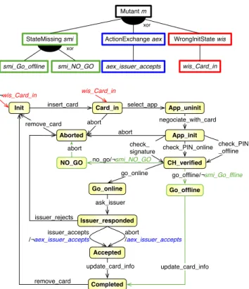
ex-ample of FD is provided at the top of Fig. 2. In this fig-ure, the root feature (m) has 3 sub-features (smi , aex , wis) connected using a xor operator. FDs have their seman-tics defined in terms of valid products, i.e., legal combi-nations of features. In the FD of Fig. 2, a valid prod-uct is {m, smi , smi Go offline} while the prodprod-uct {m, smi , smi Go offline, aex , aex issuer accepts} is invalid because it does not respect the xor constraints. FD semantics is formal [58] and FDs can be encoded as boolean constraints. Thus, SAT or BDD solvers are commonly used to enumerate products or to check their validity.
The main challenge in SPL engineering is to deal with the combinatorial explosion induced by the number of pos-sible products (2N for N features in the worst case). FTSs address this problem and enable the efficient behavioural model checking of SPLs [15]. FTSs are Transition Systems (TSs) where each transition is labelled with a feature ex-pression specifying which products of the SPL can execute the transition. A FTS is thus a compact representation of the behaviour of an SPL:
Definition 2 (Featured Transition System [15]). A Featured Transition System (FTS) is a tuple (S, Act, trans, init, d, γ), where: S, Act, trans are defined according to definition 1; d is an FD; γ : trans 7→ [[d]] 7→ {true, f alse} is a labelling function specifying for each transition which valid products may execute it; this function is represented as a boolean expression over the features of d; and init : S 7→ ([[d]] 7→ {true, f alse}) a total function that indicates if a state i ∈ S is an initial state for a product p ∈ [[d]], such that for every product p ∈ [[d]] there is exactly one initial state, which allows one to model mutants that change the initial state of the system.
A FTS example is provided at the bottom of Fig. 2. Tran-sition
CH verified−−−−−−−−−−−−−−−−→ Go offlinego offline/¬smi Go offline may only be executed in products with a valid configuration where the smi Go offline feature is not selected.
Init Card_in Aborted insert_card abort remove_card App_uninit select_app App_init negociate_with_card abort CH_verified check_PIN_online check_PIN _offline check_ signature Go_online Go_offline NO_GO no_go/¬smi_NO_GO
go_offline/¬smi_Go_ffline go_online abort Issuer_responded ask_issuer issuer_rejects Completed issuer_accepts /¬aex_issuer_accepts update_card_info Accepted update_card_info remove_card
StateMissing smi ActionExchange aex WrongInitState wis Mutant m xor smi_Go_offline smi_NO_GO xor aex_issuer_accepts wis_Card_in ¬wis_Card_in wis_Card_in abort /aex_issuer_accepts
Figure 2: Featured Mutant Model of Card Payment Terminal
3.
COMPACT MUTANTS MODEL
The key idea behind our approach is to represent mutants as a family of variations of the System Under Test (SUT). We model the SUT’s behaviour using a TS, called the origi-nal TS (to distinguish it from the mutant TS). It is possible to model these variants as an FTS and its corresponding FD, where each feature corresponds to one application of one mutant operator on the original TS. The FTS and the FD represents all the possible mutants of an original TS and is called the Featured Mutants Model (FMM).
For example, the FMM of Fig. 2 has an FD (at the top) with 3 mutation operators: the state missing (SMI ) oper-ator, which produces a mutant where one state is missing; the action exchange (AEX ) operator, which produces a mu-tant where one transition has its action changed (to another action); and the wrong initial state (WIS ) operator, which produces a mutant where the initial state has been set to an-other state. In this instance of the FD, the SMI operator has been applied twice (smi go offline, smi NO GO ), and the AEX and WIS operators have been applied one time each (aex issuer accepts, wis Card in). This FD represents four mutants, where at most one leaf feature is selected. The FTS at the bottom of Fig. 2 represents all the possible vari-ations, corresponding to the four mutation operators, of the original TS.
In order to derive one particular mutant (TS) from the FMM, one may use the FTS projection operator [15]. Prac-tically, this operator will first need a valid product represent-ing the desired mutant, e.g., p = {m, smi , smi Go offline}; then, each feature expression of the FTS is evaluated with features belonging to the product replaced by true, and other features replaced by false; finally, transitions with a feature
Enumerative FMM Input ts Input f tsf mm 0 a s1 a b 0 s1 a/γ1 a/γ2 b/γ3 Output tsm Output f ts0f mm 0 a s1 b b 0 s1 a/γ1 a/¬aex ∧ γ2 b/aex ∧ γ2 b/γ3
Figure 3: An example of mutation, the AEX opera-tor
expression evaluated to false (i.e., where γp = false) are re-moved from the FTS, and the initial state is set to the only state such that the feature expression on the initial tran-sition is true (i.e., where init(i, p) = true). For instance, the projection of the FMM of Fig. 2 on p will produce the mutant TS of Fig. 1(b).
3.1
Building the Featured Mutants Model
We rely on the state-of-the-art operators proposed by Fab-bri et al. [22] to generate mutants from a TS:
SMI State Missing operator removes a state (other than the initial state) and all its incoming/outgoing transitions; WIS Wrong Initial State operator changes the initial state; AEX Action Exchange operator replaces the action linked
to a given transition by another action;
AMI Action Missing operator removes an action from a transition;
TMI Transition Missing operator removes a transition; TAD Transition Add operator adds a transition between
two states;
TDE Transition Destination Exchange operator modifies the destination of a transition.
Each operator can be used to generate mutants using the enumerative approach, where each mutant is formed as a new variation of the original TS (possibly introducing non determinism with AEX and TAD operators), or using the FMM approach, where each mutant is an addition to the FD. We detail hereafter the mutant generation procedures. Enumerative approach: In the enumerative approach, each operator (op) is defined as a model transformation with input a TS (ts) representing the behaviour of the SUT. It produces another (mutant) TS (tsm) representing the result
of an operator on ts. For instance, AEX operator, shown on the left of Fig. 3, replaces the action a on transition s1
a
−→ s0
byb. Algorithm 1 details the enumerative approach where the set of mutants (muts) is produced by applying each op-erator (in Ops) with random parameters a number of times (defined for each operator by the times function) on the original TS (line 4).
Algorithm 1 Mutant generation, enumerative approach Require: ts = (S, Act, trans, i) {original TS}
Ops {the set of operators to use}
times : Op → N {function specifying for each operator the number of applications}
Ensure: return = muts {set of produced mutants} 1: muts ← ∅
2: for all op ∈ Ops do
3: for all i between 1 and times(op) do 4: muts ← muts ∪ op(random(ts)) 5: end for
6: end for 7: return muts
Algorithm 2 Mutant generation, FMM approach Require: ts = (S, Act, trans, i) {original TS}
Opsf mm {set of operators to use}
times : Opf mm→ N {function specifying for each
oper-ator the number of applications}
Ensure: f mm = (f tsf mm, f df mm) {FMM representing
the mutants} 1: γ ← (λt → true)
2: f tsf mm← (S, Act, trans, i, f df mm, γ)
3: f df mm← (m) {initialised to root feature m}
4: for all opf mm∈ Ops do
5: for all i between 1 and times(op) do 6: f mm ← opf mm(f mm)
7: end for 8: end for 9: return f mm
FMM approach: In the FMM approach, an operator (Opf mm) is defined as a model transformation of a FMM
(representing existing mutants), that produces a FMM rep-resenting (the previously existing mutants and) the result of the Opf mm mutation on the original TS (obtained in
the FMM’s FTS by replacing the features by false in the feature expressions). For instance, on the right of Fig. 3, the AEXf mm operator replaces the action a on transition
s1 a
−→ s0 of the base model bybas follows:
1. adding the feature expression ¬aex on transition s1 a/γ2
−−−→ s0, stating that s1
a/¬aex ∧γ2
−−−−−−−→ s0 may be fired
only if the aex mutation is inactive (and if γ2 is true);
2. adding a transition s1
b/aex ∧γ2
−−−−−−→ s0, stating that the
transition is fired with a b action only if the aex mu-tation is active (and if γ2 is true);
3. adding an aex feature to f df mmrepresenting the
mu-tation done by Opf mm(not shown in Fig. 3).
Algorithm 2 details the automated FMM building approach. We start with the original TS (line 2) and a γ function that labels each transition with a true feature expression (line 1). We then apply mutation operators (Opsf mm) a
spec-ified number of times (times(op) line 5). Contrary to the enumerative approach, the mutation operators are applied on the FMM under construction, which is reused in the next iteration (line 6). This is mandatory as the FMM contains all the previous mutations that are taken into account in the model transformations (e.g., the γiexpressions in Fig. 3). As
we choose to only perform Opf mmmutations on the original
Algorithm 3 FMM mutant execution
Require: f mm = (f tsf mm, f df mm) {FMM model}
tc = (α1, ..., αn) {test case defined over the original TS}
Ensure: live {feature expression representing the mutants live after executing tc}
1: live ← f alse
2: paths ← {(iα−→ . . .1/γ1 αn/γn
−→ i)} {paths in f tsf mm}
3: for all p ∈ paths do 4: live ← live ∨ (V
γi∈pγi)
5: end for 6: return live
TS, this forbids operator composition on (previously) mu-tated elements. Doing so ensures that first-order mutation maps to only one edit of the original TS. Further details about the operators and specificities of the transformations can be found on the VIBeS website [17] in a technical note.
3.2
Featured Mutants Model Execution
In our context, test cases are defined as a sequence of actions in a TS (ts), such that one execution form a path starting from and ending at the initial state (i) [20]: tc = (α1, ..., αn) such that ∃(i
α1
−→ sk, ..., sl αn
−→ i). Recall that in the enumerative approach, if a test case cannot be executed by the mutant (denoted m;) or does not end in the initialtc state (considered as the accepting state), it is considered killed. Otherwise, the mutant is considered live. The set of live mutants, according to tc and the mutant set muts, is defined as:
liveEnum(muts, tc) = {m ∈ muts | m=⇒}tc In the FMM approach, a test case can be executed on an FMM’s (f mm) FTS (noted f tsf mm
tc
=⇒), if there exists at least one mutant able to execute it. The enumerative ap-proach executes each test case on each mutant separately. In contrast, one execution of a test case on the FMM ex-plores all the reachable mutants (identified by the collected feature expression γ). The set of live mutants in the FMM approach is defined as:
liveFMM (f mm, tc) = {p ∈ [[f df mm]] | f ts |p f mm
tc
=⇒} Concretely, all possible paths in f tsf mmstarting from i and
ending in i will be considered, which allows to deal with possible non-determinism introduced by a mutation. The live mutants are those able to execute at least one of those paths, i.e., those for which the product p satisfies all the feature expressions on the transitions of the considered path. For instance, the test case:
tc =(insert card , select app, negociate with card , check PIN offline, go offline, update card info, remove card )
Executing the FMM of Fig. 2, it will fire the following transitions:
(−−−−−−−−−→ Init , Init/¬wis Card in −−−−−−→ Card in,insert card Card in−−−−−−→ App uninit ,select app App uninit−negociate with card−−−−−−−−−−−→ App init , App init −check PIN offline−−−−−−−−−−→ CH verified , CH verified−−−−−−−−−−−−−−−−→ Go offline,go offline/¬smi go offline
Go offline−−−−−−−−−−→ Completed ,update card info
Completed−−−−−−−→ Init )remove card These transitions may only be fired by mutants for which all the features expressions are true. In such a case, mutants need to respect the following constraint:
¬wis Card in ∧ ¬smi go offline
All mutants in the FD of Fig. 2 that satisfy this feature expression remain live after the execution of tc. The set of mutants killed by the test case is computed using the conjunction of f df mm and the negation of this feature
ex-pression: f df mm∧ (wis Card in ∨ smi go offline), which
corresponds to the set of mutants:
{(m, wis, wis Card in), (m, smi , smi go offline)} In practice, liveFMM (f mm, tc) will produce a feature ex-pression representing all the live mutants as detailed in Al-gorithm 3. Initially, the alAl-gorithm computes all the paths in f tsf mm corresponding to the sequence of actions in tc (line
2). For one path, the conjunction of the feature expressions gives the mutants able to execute this path (line 4). Effort is saved this way by ignoring unreachable mutants and by sharing the execution of the common transitions. This con-junction disjuncts with the concon-junctions of the others paths to get the feature expression representing all the live mu-tants (line 4). This step results in savings due to merging of the considered executions. For performance reasons, the paths variable uses a tree representation to merge common prefixes of different paths.
We implemented the different mutant operators described in Section 3.1 in order to perform classical mutation test-ing (enumerative approach) as well as FMM generation and execution in VIBeS, our Variability Intensive Behavioural teSting Java framework [17].
3.3
FMMs as Higher-Order Mutants Model
Higher-order mutants can be valuable since some of them tend to be hard to kill [25]. However, the number of mutants grows exponentially according to the order n and explode the involved cost. This is obvious in Algorithm 1, for the enumerative approach, which generates all the n−1 mutants to generate the n-order ones.
Using the FMM approach, modelling higher-order muta-tion comes at (nearly) no cost. In a FMM (f tsf mm, f df mm),
the set of allowed mutants (i.e., variations in f tsf mm) is
rep-resented by the feature diagram (f df mm). For instance, the
constraints in the f df mmof Fig. 2 allows to have exactly one
mutant at a time. Meaning that all valid mutants (products) of this FMM will have at most one variation from the orig-inal TS made by a mutation operator, e.g., Fig. 1(b) has
Figure 4: The Order 2 FMM of the CPT Example (only) smi go offline feature active. The n order mutants are represented by modifying the constraints on the f df mm
so that they have exactly n mutations at a time. It means that generating the FMM using Algorithm 2 will also gener-ate the FTS (which will be the same) for order 1 to n FMMs. For instance, the card payment terminal has the same FTS, for all orders as shown in Fig. 2, but differ on the FD that is described by Fig. 4 by the group cardinality stating that exactly 2 subfeatures have to be selected. The FMM will compactly represent all the C4
2 = 6 2-order mutants.
All-order mutants: Using the same argument, we gen-eralize to higher-order mutants. In this case, the FMM represents a single model with all possible n orders of tants (with n between 1 and the number of possible mu-tants which is the number of leaf features in the FMM’s FD). By setting the group cardinalities of the FD in Fig. 4 to [1..∗]. A valid product (mutant) of the FD will contain at least one applications of mutation operator, e.g., a product p = {m, smi go offline}, but also p0 = {m, smi go offline, smi NO GO }, or p00 = {m, smi go offline, wis Card in}, etc. In this case, the FMM compactly represent all the P4
k=1C 4
k = 15 n-order mutants. The number of live
mu-tants after the execution of a test case (tc) on a FMM (f mm) can be obtained by counting the number of SAT solutions (i.e., the number of possible assignments for each feature) to f df mm∧ liveFMM (f mm, tc). Where f df mm is the FMM’s
FD encoded as a boolean formula, i.e., the disjunction of the mutation operator (Ops): f df mm = Wo∈Opso. For a
test set (ts), the number of live mutants is computed by counting the number of SAT solutions to
_ o∈Ops o ! ∧ ^ tc∈ts liveFMM (f mm, tc) ! .
4.
EVALUATION
We formulate our research questions as follows:
RQ1 How does the FMM scheme compare with the “enumer-ative approach” in terms of execution time ?
RQ2 Is higher-order mutation under the FMM scheme trac-table?
4.1
Setup
We compare two test execution approaches: the enumer-ative approach, which is the classical mutation testing ap-proach used by previous research [2] where each test case is executed against each mutant, and the FMM approach, where each test case is executed (only once) on the FMM. Models: We consider models from different sources with varying size. Table 2 details the employed models. For each model, we measure: the number of states (States); the num-ber of transitions (Trans.); the numnum-ber of actions (Act.); the average degree of the different states that correspond to the average number of incoming or outgoing transitions per
Table 2: Models characteristics
Model States Trans. Act. Avg. deg. BFS height Back lvl tr. S. V. Mach. 9 13 14 1.44 5 3 Minepump 25 41 23 4.64 15 9 Claroline 106 2055 106 19.37 1 105 AGE-RR 772 6,639 772 8.60 328 408 Elsa-RR 384 1,214 384 3.16 194 174 Elsa-RRN 615 1,771 615 2.88 369 289 Random 10,000 13,652 120 1.37 7,924 3,303
state (Avg. deg.); the maximal number of states between the initial state and another state when traversing the TS in breadth-first search (BFS height ); the number of transi-tions starting from a state and ending in another state with a lower level when traversing the TS in breadth-first search (Back lvl tr.).
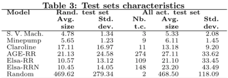
Our models are: the soda vending machine model (S. V. Mach.) which is a small example modelling the behaviour of a machine selling soda and tea [14]; the mine pump (Mine-pump) that models the behaviour of a pump which has to keep a mine safe from flooding by pumping water from a sink while avoiding methane explosions [14]; the Claroline website (Claroline) that represents the navigational usages of the online course management platform used at the Uni-versity of Namur (http://webcampus.fundp.ac.be). It has been reverse-engineered from an Apache log using a 2-gram inference method [19, 59]; the WordPress models (AGE-RR, Elsa-RR, and Elsa-RRN ) that represent the navigational usage of two different WordPress instances. They are also reverse-engineered using a 2-gram inference method. For the AGE-RR and Elsa-RR, we considered only the request type (e.g., POST, GET, HEAD) and the requested resource (e.g., “/index.php”) in the sequences used. For the Elsa-RRN model, we considered the request type, the requested resource and the parameter names (e.g., “?page=”) in the se-quences used as input of the 2-gram inference method [59]. The random model has been generated based on the fol-lowing procedure: a) we generate a set of random graphs (basically directed arcs and nodes) and compute the differ-ent measures from Table 2 (except number of actions) on them; b) we selected those graphs that are likely to rep-resent a real system according to Pel´anek [56], i.e., those having a small average degree, a large BFS height and a small number of back level edges (in this order); c) we ap-plied a random labelling multiple times and computed the occurrence probability, i.e., the probability of the labels to obtain a set of randomly generated TSs; d) we selected the TS that had the following properties1: the probability of the most occurring label in the TS was less than or equal to 6%, and the cumulated probability of the 5 most frequently occurring labels was less than or equal to 20% [57]; e) we ended up with one random model as recorded in Table 2. Test Cases: For every model, we generate one set of tests using random walks on the TS and one set satisfying the all-actions criterion. The test sets were then executed with the enumerative and the FMM processes. Table 3 records the average size (and standard deviation) of the randomly generated test cases, the size of the generated all-actions coverage-driven test set and the average size (and standard
1
These properties are likely to represent real systems [56]
Table 3: Test sets characteristics
Model Rand. test set All act. test set
Avg. size Std. dev. Nb. t.c. Avg. size Std. dev. S. V. Mach. 4.78 1.34 3 5.33 2.08 Minepump 5.65 1.23 9 6.11 1.45 Claroline 17.11 16.97 11 13.18 9.20 AGE-RR 21.13 24.58 274 27.11 33.62 Elsa-RR 10.57 13.12 109 21.10 33.45 Elsa-RRN 10.45 14.05 148 23.20 43.49 Random 469.62 279.34 2 468.50 118.09
Table 4: Mutant operators
Model WIS TMI AEX TDE TAD AMI SMI Total
S. V. Mach. 1 1 1 1 1 1 1 7 Minepump 2 4 4 4 4 3 2 23 Claroline 9 188 205 204 205 189 9 1,009 AGE-RR 73 525 663 663 663 516 75 3,178 Elsa-RR 36 102 121 121 121 106 38 645 Elsa-RRN 57 153 177 177 177 155 57 953 Random 942 1,276 1,365 1,365 1,365 1,295 954 8,562
deviation) of its test cases. The size of the random test set is arbitrarily fixed to 100 test cases.
Model Mutants: We used the operators presented in Section 3.1. Operators modifying states (WIS and SMI ) or transitions (TMI, AEX, TDE, TAD, and AMI ), resp., were applied arbitrarily for 1/10 of the number of states or transitions, resp., in the model (with 1 as bottom value). Since the operands are randomly chosen, we forbid multiple applications of any operator on the same operands to avoid duplicated mutants [52]. Table 4 presents the number of mutants generated per operator for the studied models. Mutant Execution: To avoid execution time bias from the underlying machines, we execute each test case 3 times with each considered mutant (for the enumerative version) and on the FMM (for the family version).
Experimentation was performed on an Ubuntu 14.04 LTS Linux (kernel 3.13) machine with Intel Core i3 (3.10GHz) processor and 4GB of memory. The complete experiment took approximately 2 weeks.
4.2
Results and Discussion
Fig. 5 presents the distribution of the test execution time (in logarithmic scale on the y axis) for each studied model with a box plot. The first two columns represent the to-tal execution time taken by each test case when executed on the live mutants and on the killed mutants according to the enumerative approach. The third box presents the execution time of the FMM (FMM approach). Note that while the killed mutants do not require a complete execu-tion in the enumerative approach, it is required for the FMM mutants. This might provide an advantage to the enumer-ative approach. To assess this, we consider the killed and the live mutants separately. In all cases, we measure only the execution of the models, avoiding time bias due to I/O operations. As the execution time of a test case partially depends on its size, the high number of outliers in Fig. 5 is explained by the variation of the test cases sizes. Tables 5 and 6 record different statistics over the execution time of the models in µ-seconds. For the enumerative approach, executing a test case on mutants that will remain live takes more time than executing the same test cases on mutants that are killed. This was expected since killed mutants do
● ● ● Live Killed FMM 20 50 100 200 500
S. V. Mach.
Time (in microsec.)
● ● ● ● Live Killed FMM 50 100 200 500
Minepump
● ● ● ● ● ● ● ● ● ● ● ● ● ● ● ● ● ● ● ● ● ● ● ● ● ● ● ● ● ● ● ● ● ● ● ● ● ● ● ● ● ● ● ● ● ● ● ● ● ● ● ● ● ● ● ● ● ● ● ● ● ● ● ● ● ● ● ● ● ● ● ● ● ● ● ● ● ● ● ● ● ● ● ● ● ● ● ● ● ● ● ● ● ● ● ● ● ● ● ● ● ● ● ● ● ● ● ● ● ● ● ● ● ● ● ● ● ● ● ● ● ● ● ● ● ● ● ● ● ● ● ● ● ● ● ● ● ● ● ● ● ● ● Live Killed FMM 5e+01 5e+02 5e+03 5e+04Claroline
● ● ● ● ● ● ● ● ● ● ● ● ● ● ● ● ● ● ● ● ● ● ● ● ● ● ● ● ● ● ● ● ● ● ● ● ● ● ● ● ● ● ● ● ● ● ● ● ● ● ● ● ● ● ● ● ● ● ● ● ● ● ● ● ● ● ● ● ● ● ● ● ● ● ● ● ● ● ● ● ● ● ● ● ● ● ● ● ● ● ● ● ● ● ● ● ● ● ● ● ● ● ● ● ● ● ● ● ● ● ● ● ● ● ● ● ● ● ● ● ● ● ● ● ● ● ● ● ● ● ● ● ● ● ● ● ● ● ● ● ● ● ● ● ● ● ● ● ● ● ● ● ● ● ● ● ● ● ● ● ● ● ● ● ● ● ● ● ● ● ● ● ● ● ● ● ● ● ● ● ● ● ● ● ● ● ● ● ● ● ● ● ● ● ● ● ● ● ● ● ● ● ● ● ● ● ● ● ● ● ● ● ● ● ● ● ● ● ● ● ● ● ● ● ● ● ● ● ● ● ● ● ● ● ● ● ● ● ● ● ● ● ● ● ● ● ● ● ● ● ● ● ● ● ● ● ● ● ● ● ● ● ● ● ● ● ● ● ● ● ● ● ● ● ● ● ● ● ● ● ● ● ● ● ● ● ● ● ● ● ● ● ● ● ● ● ● ● ● ● ● ● ● ● ● ● ● ● ● ● ● ● ● ● ● ● ● ● ● ● ● ● ● ● ● ● ● ● ● ● ● ● ● ● ● ● ● ● ● ● ● ● ● ● ● ● ● ● ● ● ● ● ● ● ● ● ● ● ● ● ● ● ● ● ● ● ● ● ● ● ● ● ● ● ● ● ● ● ● ● ● ● ● ● Live Killed FMM 1e+02 1e+04 1e+06AGE−RR
● ● ● ● ● ● ● ● ● ● ● ● ● ● ● ● ● ● ● ● ● ● ● ● ● ● ● ● ● ● ● ● ● ● ● ● ● ● ● ● ● ● ● ● ● ● ● ● ● ● ● ● ● ● ● ● ● ● ● ● ● ● ● ● ● ● ● ● ● ● ● ● ● ● ● ● ● ● ● ● ● ● ● ● ● ● ● ● ● ● ● ● ● ● ● ● ● ● ● ● ● ● ● ● ● ● ● ● ● ● ● ● ● ● ● Live Killed FMM 100 500 2000 10000 50000Elsa−RR
Time (in microsec.)
● ● ● ● ● ● ● ● ● ● ● ● ● ● ● ● ● ● ● ● ● ● ● ● ● ● ● ● ● ● ● ● ● ● ● ● ● ● ● ● ● ● ● ● ● ● ● ● ● ● ● ● ● ● ● ● ● ● ● ● ● ● ● ● ● ● ● ● ● ● ● ● ● ● ● ● ● ● ● ● ● ● ● ● ● ● ● ● ● ● ● ● ● ● ● ● ● ● ● ● ● ● ● ● ● ● ● ● ● ● ● ● Live Killed FMM 1e+02 1e+03 1e+04 1e+05
Elsa−RRN
● ● ● ● ● ● ● ● ● ● ● ● ● Live Killed FMM 1e+03 1e+04 1e+05 1e+06Random
Figure 5: Execution Time: time required by a test case to execute with live, killed mutants and the FMM mutants, time is measured in µsec..
not require a complete execution of the test case. In both cases, the FMM execution runs faster, i.e., running a test case on all the mutants at once is very fast, despite the more complex (needed) exploration of the FMM’s FTS.
Regarding RQ1, the box plots of Fig. 5 and the values of Tables 5 and 6 confirm that the execution time required by the FMM approach is considerably lower than the time required by the enumerative approach. The difference esca-lates to several orders of magnitude when considering live mutants. The difference between family-based and enumer-ative approaches increases with the size of the model, indi-cating the improved scalability of our approach.
To evaluate the statistical significance, we use a Wilcoxon rank-sum test for the different models we considered: we obtain a p-value of 1.343e − 09 for the random model and p-values smaller than 2.2e−16 for the other models, confirm-ing the hypothesis that FMM significantly outperforms the enumerative approach, when considering 0.001 significance level.
4.2.1
All-Order Mutation
Table 7 presents the number of all-order mutants for our models, the number of mutants live after executing the ran-dom and all-actions test sets (computed using SAT4J 2.3.5),
and their mutation score. Mem. Overflow denotes an over-flow during SAT solving, improving this step by, for instance, reducing the boolean formula to process is part of our future work. Columns 5 and 8 give the SAT-solving computation time (we set a timeout of 12 hours).
Overall, our results suggest that higher-order mutation under the FMM scheme is tractable, answering positively to RQ2. In particular, all-order mutation achieves very good mutation scores (M S ≥ 0.99) when compared to first-order mutation when this score can be computed. In our future work, we intend to: (i) improve the scalability of mutation score computation; and (ii) assess the practical relevance of higher-order in test sets comparison.
Only one mutant is live for the soda vending machine and the mine pump models. This mutant is a first order mutant resulting from the TAD operator. Indeed, the TAD operator adds new transition which cannot be detected by test cases solely generated from the original TS, since this transition does not exist in this model. All-order mutation enables to quickly kill mutants of any order an to focus on the interesting ones from a selective mutation perspective. For example, the 2916 remaining live mutants resulting from the execution of the all-action test suite are relevant to study the mutation operators involved. Of course, they can also be
Table 5: Mutant (1st order) execution time in µ-seconds: minimal, maximal, median, mean, standard devia-tion for every test case on all live and killed mutants of the enumerative method and of the FMM. Mutadevia-tion score (MS) of the all actions and random test sets are provided for each model.
S. V. Mach. model (all act. MS: 0.85 ; random MS: 0.85 )
Live m. Killed m. FMM Speedup
Min. 57 21 20 1.1
Max. 442 154 83 5.3
Median 113 79 38 2.5
Mean 120 78 39 2.5
S.Dev. 43 35 7.1 6.1
Minepump model (all act. MS: 0.60 ; random MS: 0.82 )
Live m. Killed m. FMM Speedup
Min. 441 43 26 1.7
Max. 623 212 64 9.7
Median 533 108 41 8
Mean 530 100 42 7.6
S.Dev. 35 49 6.5 34
Claroline model (all act. MS: 0.07 ; random MS: 0.27 )
Live m. Killed m. FMM Speedup
Min. 40,314 236 26 9.1
Max. 103,346 4,091 19,282 5.4
Median 53,951 652 58 380
Mean 57,000 870 280 100
S.Dev. 13,000 710 1,400 22
AGE-RR model (all act. MS: 0.66 ; random MS: 0.27 )
Live m. Killed m. FMM Speedup
Min. 598,520 5,644 39 140
Max. 3,948,806 99,754 46,839 84
Median 910,000 9000 110 3,300
Mean 1.1e+06 14,000 200 2,900
S.Dev. 590,000 12,000 790 870
Elsa-RR model (all act. MS: 0.75 ; random MS: 0.49 )
Live m. Killed m. FMM Speedup
Min. 20,743 775 104 7.5
Max. 59,237 13,400 3,109 19
Median 22,676 918 191 89
Mean 27,000 1,300 230 62
S.Dev. 8,500 1,500 170 84
Elsa-RRN model (all act. MS: 0.77 ; random MS: 0.30 )
Live m. Killed m. FMM Speedup
Min. 34,999 1,286 93 14
Max. 166,433 34,498 36,158 4.6
Median 45,000 1,600 180 200
Mean 52,000 2,400 300 90
S.Dev. 17,000 3,200 1,600 17
Table 6: Mutant execution time in µ-seconds
Random Model (all act. MS: 0.16 ; random MS: 0.63 )
Live m. Killed m. FMM Speedup
Min. 327,418 24,675 875 28
Max. 2,552,363 140,917 60,354 42
Median 1.3e+06 55,000 1,500 160
Mean 1.3e+06 63,000 1,800 370
S.Dev. 560,000 29,000 3,500 210
Table 7: All-order mutation score. For each test set and model, the table records the number of possible mutants (# mut.), the number of live mutants after the test set execution (#Lv.), the mutations score (MS) and the SAT computation time (T) in seconds.
Model # mut. All act. Rand
#Lv. MS T #Lv. MS T
S. V. Mach. 127 1 0.99 1.10 1 0.99 17.67 Minepump 8,388,607 1 >0.99 1.84 1 >0.99 15.72 Claroline 5.49e+303 Timeout Timeout AGE-RR 4.71e+956 Timeout Timeout Elsa-RR 1.46e+194 2916 >0.99 37.78 144 >0.99 10.19 Elsa-RRN 7.61e+286 36 >0.99 150.32 16 >0.99 83.04 Random 2.62e+2577 Mem. overflow Mem. overflow
used to generate test cases killing them in order to augment the test suite. Exploring all-order MS in selective mutation or test case generation scenarios are part of our future work.
4.2.2
Threats to Validity
Internal Validity: Our experiments were performed on 7 models: 2 academic examples (the soda vending machine and the the mine pump), 4 larger real-world models (Claro-line, AGE-RR, Elsa-RR, and Elsa-RRN) and a randomly generated one. These models come from different sources and represent different kinds of systems: embedded systems designed by an engineer and web-based applications where the model has been reverse-engineered from a running
in-stance. The random model was built upon a set of generated TSs in order to match the real system state-space measures, as described by Pel´anek [56, 57].
Construct Validity: We chose to apply mutants for 1/10 of the states and/or transitions of the mutated model. This might result in more (or less) mutants than needed for the larger models. However, this is expected when using mu-tation. Additionally, since model-based mutation is applied to the system’s abstraction, abstract actions represent many concrete actions. It is therefore important to ensure a good coverage of most of the model actions.
TS and FTS executions are different, and do not use the same algorithms. In order to decrease the bias in measuring execution time, both executions of the models have been done using VIBeS [17], our Variability Intensive Behavioural teSting framework Java implementation. The two execution classes are different but use a variant of the same algorithm described in Section 3.2. Moreover, we used the Stopwatch Java class to measure the call to the execute method (i.e., model loading and result writing time have been omitted). Finally, we ran each test case 3 times on each mutant model (classical and FTS) to avoid bias due to process concurrency. External Validity: We cannot guarantee that our re-sults are generalizable to all behavioural models. However, we recall the diversity of the model sources (hand-crafted, reverse-engineered, and randomly generated to match real system state-space) as well as the diversity of considered systems.
5.
RELATED WORK
Program mutation was proposed as a rigorous testing tech-nique [12]. The idea was then applied to test specifica-tion models [50] and recently to resolve software engineering problems such as the improvement of non-functional proper-ties [42], locating [53] and fixing software defects [43]. Here we briefly discuss works related to model-based mutation and testing, and code-based mutation.
5.1
Model-Based Mutation
The idea of model-based mutation has been elicited by Gopal and Budd [13] who called it “Specification Mutation”. Specification mutation promises to identify defects related to missing functionality and misinterpreted specifications [13]. This is desirable since these kinds of defects cannot be iden-tified by any code-based testing technique [28, 62], including code-based mutation.
Gopal and Budd [13] studied mutation for specifications expressed in logic. Similarly, Woodward [63] mutated and experimented with algebraic specifications. Mutating mod-els like finite state machines and Statecharts has also been done by Fabbri et al. [21]. Hierons and Merayo [27] used Probabilistic Finite State Machines. All these studies sug-gested a set of operators and report some exploratory re-sults. Amman et al. [4] suggested comparing the original and the mutated specification models using a model checker in order to generate counterexamples. These can then be used as test cases for the system under test. Black et al. [10] defined a set of operators based on empirical and theoretical analysis. They also defined a process of using them based on the SMV model checker. Contrary to our approach, none of these methods considers the mutation efficiency.
Recent research focuses on mutating behavioural models. Aichernig et al. [2, 3] defined UML state machines mutant operators and used them to insert faults in the models of an industrial system. These were used to design tests. The approach has a formal ground but neither considers optimis-ing the test execution, nor higher-order mutation. Belli and Beyazit [8, 9] compare event-based and state-based model mutation testing. Both approaches were found to have simi-lar fault detection capabilities. The authors also report that it seems more promising to perform higher-order mutation than first-order mutation but did not provide evidence in support of this argument. Krenn et al. [39] made available their MoMuT tool, but it is dedicated to test generation and not mutant execution as our approach. In their most recent work [38], they use an idea similar to FMM by triggering mutations during exploration of the model, avoiding execu-tion of similar prefixes in different mutants. Addiexecu-tionally, MoMut does not support higher-order mutation.
Other applications of model-based mutation are to test model transformations and test configurations. Mottu et al. [47] defined a fault model relevant to the model transfor-mation process based on which they propose a set of mutant operators. Henard et al. [26] define mutant operators for fea-ture models. Along the same lines, Lackner and Schmidt [40] define mutant operators for the mappings of features with other model artifacts. Finally, Papadakis et al. [51] demon-strated that model-based mutation of the combinatorial in-teraction testing models has a higher correlation with the actual fault detection than the use of combinatorial interac-tion testing. Thereby, they provide ground to the argument that model-based mutation might be more effective than the other model-based testing methods.
5.2
Model-Based Testing
Offutt et al. [49] define test criteria for state-based spec-ifications. They also describe techniques to automatically generate tests based on these criteria. Lackner et al. [41] suggested a test generation approach for product lines. Sim-ilar to our work they combine feature diagrams with state machines to handle the product line variability. However,
their approach does not perform mutation and it is specific to software product lines. Briand et al. [11] proposed a tech-nique for generating tests from statecharts. Their results were validated through code-based mutation.
5.3
Code-Based Mutation
In the context of code-based mutation, executable mu-tants are needed. This introduces a compilation overhead which is proportional to the number of mutants. To reduce this cost, Untch et al. [60] proposed mutant schemata, an ap-proach that replaces the program operators with schematic functions. These functions introduce the mutants at run-time and thus, only one compilation is needed. Ma et al. [45] suggested using bytecode translation, a technique that intro-duces the mutants directly at the bytecode level and thus avoid multiple compilations.
To reduce the test execution overhead, several optimiza-tions have been proposed. Delamaro and Maldonado [16] suggested recording the execution trace of the original pro-gram and consider only the mutants that are reachable by each of the employed tests. Along the same lines, Mateo and Polo [46] suggested stopping mutant executions when they cause infinite loops. Jackson and Woodward [29] sug-gested parallelizing the mutant execution process. Kapoor and Bowen [35] proposed ordering the mutants in such a way that the test execution is minimized. Papadakis and Malevris [55] used mutant schemata to identify mutants that are reached and infected by the considered tests. They then reduce test execution by considering only the mutants that cause infection. This technique was later evaluated by Just et al. [32] who found that it reduces test execution by 40%.
6.
CONCLUSION
This paper presents a family-based approach to model-based mutation testing, named Featured Mutant Model. It allows to generate mutants of any order and assess test ef-fectiveness via an optimised execution scheme. Testing be-havioural models with FMM is a completely automated pro-cess that involves no extra manual or computational effort over previous approaches.
In short, the use of FMM has the following benefits: (i) it can easily reason about and generate behavioural mutants, (ii) it can significantly speed up the evaluation of test suites against mutants (up to 1,000 times) and (iii) it can effi-ciently perform higher-order mutation. But, obviously, this is not the end of the story.
In our future work, we will further investigate scalability issues regarding all-order mutation analysis to be able to compute mutation score for the largest models. This implies the optimisation of the boolean formulas or approximate computation heuristics. Finally, since “mutants are a valid substitute for real faults” [33], we envision to develop test case generation techniques based on mutation coverage of the FMM.
Acknowledgements
The authors would like to thank Maxime Cordy, Bernhard Aichernig, and the reviewers for their helpful comments, the AGE (University of Namur) and the Elsa organisation for providing logs of WordPress sites. This research was partly funded by Walloon region under the INOGRAMS project (n◦7171). Mike Papadakis is supported by the National Re-search Fund, Luxembourg, INTER/MOBILITY/14/7562175.
7.
REFERENCES
[1] B. K. Aichernig, J. Auer, E. J¨obstl, R. Korosec, W. Krenn, R. Schlick, and B. V. Schmidt. Model-based mutation testing of an industrial
measurement device. In Tests and Proofs, volume 8570 of LNCS, pages 1–19. Springer, 2014.
[2] B. K. Aichernig, H. Brandl, E. J¨obstl, W. Krenn, R. Schlick, and S. Tiran. Killing strategies for model-based mutation testing. Software Testing, Verification and Reliability, 2014.
[3] B. K. Aichernig, E. J¨obstl, and S. Tiran. Model-based mutation testing via symbolic refinement checking. Science of Computer Programming, 97:383–404, Jan. 2015.
[4] P. E. Ammann, P. E. Black, and W. Majurski. Using model checking to generate tests from specifications. In ICFEM, pages 46–54. IEEE, 1998.
[5] J. H. Andrews, L. C. Briand, Y. Labiche, and A. S. Namin. Using Mutation Analysis for Assessing and Comparing Testing Coverage Criteria. Software Engineering, IEEE Transactions on, 32(8):608–624, 2006.
[6] C. Baier and J. Katoen. Principles of model checking. MIT Press, 2008.
[7] R. Baker and I. Habli. An empirical evaluation of mutation testing for improving the test quality of safety-critical software. IEEE Transactions on Software Engineering, 39(6):787–805, 2013. [8] F. Belli and M. Beyazit. Event-Based Mutation
Testing vs. State-Based Mutation Testing - An Experimental Comparison. In COMPSAC, pages 650–655. IEEE, July 2011.
[9] F. Belli, C. J. Budnik, and W. E. Wong. Basic Operations for Generating Behavioral Mutants. In Proceedings of the Second Workshop on Mutation Analysis. IEEE, Nov. 2006.
[10] P. E. Black, V. Okun, and Y. Yesha. Mutation operators for specifications. In ASE. IEEE, 2000. [11] L. C. Briand, M. D. Penta, and Y. Labiche. Assessing
and improving state-based class testing: A series of experiments. IEEE Transactions on Software Engineering, 30(11):770–793, 2004.
[12] T. A. Budd. Mutation Analysis of Program Test Data. PhD thesis, Yale University, New Haven, CT, USA, 1980. AAI8025191.
[13] T. A. Budd and A. S. Gopal. Program testing by specification mutation. Computer Languages, 10(1):63–73, Jan. 1985.
[14] A. Classen. Modelling with FTS: a Collection of Illustrative Examples. Technical Report P-CS-TR SPLMC-00000001, PReCISE Research Center, University of Namur, Namur, Belgium, 2010. [15] A. Classen, M. Cordy, P.-Y. Schobbens, P. Heymans,
A. Legay, and J.-F. Raskin. Featured Transition Systems: Foundations for Verifying
Variability-Intensive Systems and Their Application to LTL Model Checking. IEEE Transactions on Software Engineering, 39(8):1069–1089, Aug. 2013.
[16] M. E. Delamaro and J. C. Maldonado. Proteum/im 2.0: An integrated mutation testing environment. In W. E. Wong, editor, Mutation Testing for the New Century, pages 91–101. Kluwer Academic Publishers, Norwell, MA, USA, 2001.
[17] X. Devroey and G. Perrouin. Variability Intensive system Behavioural teSting (VIBeS) v. 1.0.1. https://projects.info.unamur.be/vibes/, 2015. [18] X. Devroey, G. Perrouin, M. Cordy, M. Papadakis,
A. Legay, and P.-Y. Schobbens. A Variability Perspective of Mutation Analysis. In FSE, pages 841–844. ACM, 2014.
[19] X. Devroey, G. Perrouin, M. Cordy, H. Samih, A. Legay, P.-Y. Schobbens, and P. Heymans. Statistical prioritization for software product line testing: an experience report. Software & Systems Modeling, pages 1–19, 2015.
[20] X. Devroey, G. Perrouin, A. Legay, M. Cordy, P.-Y. Schobbens, and P. Heymans. Coverage Criteria for Behavioural Testing of Software Product Lines. In ISoLA, volume 8802 of LNCS, pages 336–350. Springer, 2014.
[21] S. Fabbri, J. C. Maldonado, and M. E. Delamaro. Proteum/FSM: a tool to support finite state machine validation based on mutation testing. In SCCC, pages 96–104. IEEE, 1999.
[22] S. Fabbri, J. C. Maldonado, T. Sugeta, and P. C. Masiero. Mutation testing applied to validate specifications based on statecharts. In ISSRE, pages 210–219. IEEE, 1999.
[23] G. Fraser and A. Arcuri. Achieving scalable mutation-based generation of whole test suites. Empirical Software Engineering, pages 1–30, 2014. [24] M. Gligoric, A. Groce, C. Zhang, R. Sharma, M. A.
Alipour, and D. Marinov. Comparing non-adequate test suites using coverage criteria. In ISSTA, pages 302–313. ACM, 2013.
[25] M. Harman, Y. Jia, P. Reales Mateo, and M. Polo. Angels and monsters: An empirical investigation of potential test effectiveness and efficiency improvement from strongly subsuming higher order mutation. In ASE, pages 397–408. ACM, 2014.
[26] C. Henard, M. Papadakis, G. Perrouin, J. Klein, and Y. Le Traon. Assessing software product line testing via model-based mutation: An application to similarity testing. In ICST, pages 188–197. IEEE, 2013.
[27] R. M. Hierons and M. G. Merayo. Mutation testing from probabilistic and stochastic finite state machines. Journal of Systems and Software, 82(11):1804–1818, 2009.
[28] W. E. Howden. Reliability of the path analysis testing strategy. IEEE Transactions on Software Engineering, 2(3):208–215, 1976.
[29] D. Jackson and M. R. Woodward. Parallel firm mutation of java programs. In W. E. Wong, editor, Mutation Testing for the New Century, pages 55–61. Kluwer Academic Publishers, Norwell, MA, USA, 2001.
[30] Y. Jia. Higher order mutation testing. PhD thesis, University College London (University of London), 2013.
[31] Y. Jia and M. Harman. An Analysis and Survey of the Development of Mutation Testing. Software
Engineering, IEEE Transactions on, 37(5):649–678, Sept. 2011.
[32] R. Just, M. D. Ernst, and G. Fraser. Efficient mutation analysis by propagating and partitioning infected execution states. In ISSTA, pages 315–326. ACM, 2014.
[33] R. Just, D. Jalali, L. Inozemtseva, M. D. Ernst, R. Holmes, and G. Fraser. Are Mutants a Valid Substitute for Real Faults in Software Testing? In FSE, pages 654–665. ACM, 2014.
[34] K. Kang, S. Cohen, J. Hess, W. Novak, and A. S. Peterson. Feature-Oriented Domain Analysis (FODA) Feasibility Study. Technical report, Carnegie-Mellon University, Software Engineering Institute, 1990. [35] K. Kapoor and J. P. Bowen. Ordering mutants to
minimise test effort in mutation testing. In FATES 2004, volume 3395 of LNCS, pages 195–209. Springer, 2004.
[36] C. H. P. Kim, S. Khurshid, and D. S. Batory. Shared execution for efficiently testing product lines. In ISSRE, pages 221–230. IEEE, 2012.
[37] C. H. P. Kim, D. Marinov, S. Khurshid, D. S. Batory, S. Souto, P. Barros, and M. d’Amorim. Splat: lightweight dynamic analysis for reducing combinatorics in testing configurable systems. In ESEC/FSE, 2013, pages 257–267. ACM, 2013. [38] W. Krenn and R. Schlick. Mutation-driven Test Case
Generation Using Short-lived Concurrent Mutants – First Results. Technical report, jan 2016.
[39] W. Krenn, R. Schlick, S. Tiran, B. Aichernig, E. Jobstl, and H. Brandl. MoMut::UML Model-Based Mutation Testing for UML. In ICST, pages 1–8. IEEE, April 2015.
[40] H. Lackner and M. Schmidt. Towards the assessment of software product line tests: A mutation system for variable systems. In SPLC Workshops, SPLC ’14, pages 62–69. ACM, 2014.
[41] H. Lackner, M. Thomas, F. Wartenberg, and
S. Weißleder. Model-based test design of product lines: Raising test design to the product line level. In ICST, pages 51–60, Cleveland, Ohio, USA, 2014. IEEE. [42] W. B. Langdon and M. Harman. Optimising existing
software with genetic programming. IEEE Transactions on Evolutionary Computation, 19(1):118–135, Feb 2015.
[43] C. Le Goues, T. Nguyen, S. Forrest, and W. Weimer. GenProg: A generic method for automatic software repair. IEEE Transactions on Software Engineering, 38(1):54–72, Jan.-Feb. 2012.
[44] N. Li and J. Offutt. A test automation language framework for behavioral models. In 2015 IEEE Eighth International Conference on Software Testing, Verification and Validation Workshops (ICSTW), number 1, pages 1–10. IEEE, apr 2015.
[45] Y. Ma, J. Offutt, and Y. R. Kwon. Mujava: an automated class mutation system. Software Testing, Verification and Reliability, 15(2):97–133, 2005. [46] P. R. Mateo and M. P. Usaola. Reducing mutation
costs through uncovered mutants. Software Testing, Verification and Reliability, 25(5-7):464–489, 2014. [47] J. Mottu, B. Baudry, and Y. Le Traon. Mutation
analysis testing for model transformations. In
ECMDA-FA, volume 4066 of LNCS, pages 376–390. Springer, 2006.
[48] H. V. Nguyen, C. K¨astner, and T. N. Nguyen. Exploring variability-aware execution for testing plugin-based web applications. In ICSE, pages 907–918. ACM, 2014.
[49] A. J. Offutt, S. Liu, A. Abdurazik, and P. Ammann. Generating test data from state-based specifications. Softwre Testing, Verification and Reliability,
13(1):25–53, 2003.
[50] J. Offutt. A mutation carol: Past, present and future. Information and Software Technology,
53(10):1098–1107, Oct. 2011.
[51] M. Papadakis, C. Henard, and Y. Le Traon. Sampling program inputs with mutation analysis: Going beyond combinatorial interaction testing. In ICST, pages 1–10. IEEE, 2014.
[52] M. Papadakis, Y. Jia, M. Harman, and Y. Le Traon. Trivial compiler equivalence: A large scale empirical study of a simple fast and effective equivalent mutant detection technique. In ICSE, pages 936–946. IEEE, 2015.
[53] M. Papadakis and Y. Le Traon. Metallaxis-FL: mutation-based fault localization. Software Testing, Verification and Reliability, 2013.
[54] M. Papadakis and N. Malevris. Automatic mutation test case generation via dynamic symbolic execution. In ISSRE, pages 121–130. IEEE, 2010.
[55] M. Papadakis and N. Malevris. Automatically performing weak mutation with the aid of symbolic execution, concolic testing and search-based testing. Software Quality Journal, 19(4):691–723, 2011. [56] R. Pel´anek. Typical Structural Properties of State
Spaces. In S. Graf and L. Mounier, editors, Model Checking Software, volume 2989 of LNCS, pages 5–22. Springer, 2004.
[57] R. Pel´anek. Properties of state spaces and their applications. International Journal on Software Tools for Technology Transfer, 10(5):443–454, 2008. [58] P.-Y. Schobbens, P. Heymans, J.-C. Trigaux, and
Y. Bontemps. Generic semantics of feature diagrams. Computer Networks, 51(2):456–479, 2007.
[59] S. E. Sprenkle, L. L. Pollock, and L. M. Simko. Configuring effective navigation models and abstract test cases for web applications by analysing user behaviour. Software Testing, Verification and Reliability, 23(6):439–464, 2013.
[60] R. H. Untch, A. J. Offutt, and M. J. Harrold. Mutation analysis using mutant schemata. In ISSTA, pages 139–148, 1993.
[61] M. Utting and B. Legeard. Practical Model-Based Testing: A Tools Approach. Morgan Kaufmann, 2007. [62] J. M. Voas and G. McGraw. Software Fault Injection: Inoculating Programs Against Errors. John Wiley & Sons, Inc., 1997.
[63] M. R. Woodward. Errors in algebraic specifications and an experimental mutation testing tool. Software Engineering Journal, 8(4):221–224, July 1993.