RESEARCH OUTPUTS / RÉSULTATS DE RECHERCHE
Author(s) - Auteur(s) :
Publication date - Date de publication :
Permanent link - Permalien :
Rights / License - Licence de droit d’auteur :
Bibliothèque Universitaire Moretus Plantin
Dépôt Institutionnel - Portail de la Recherche
researchportal.unamur.be
University of NamurModelling Built-Settlements between Remotely-Sensed Observations
Nieves, Jeremiah J.; Sorichetta, Alessandro; Linard, Catherine; Bondarenko, Maksym; Steele, Jessica; Stevens, Forrest; Gaughan, Andrea E.; Carioli, Alessandra; Clarke, Donna; Esch, Thomas; Tatem, Andrew J.
Published in: Polymer Preprints
Publication date: 2018
Document Version
Early version, also known as pre-print Link to publication
Citation for pulished version (HARVARD):
Nieves, JJ, Sorichetta, A, Linard, C, Bondarenko, M, Steele, J, Stevens, F, Gaughan, AE, Carioli, A, Clarke, D, Esch, T & Tatem, AJ 2018, 'Modelling Built-Settlements between Remotely-Sensed Observations', Polymer Preprints, vol. 2018120250. <https://www.preprints.org/manuscript/201812.0250/v1>
General rights
Copyright and moral rights for the publications made accessible in the public portal are retained by the authors and/or other copyright owners and it is a condition of accessing publications that users recognise and abide by the legal requirements associated with these rights. • Users may download and print one copy of any publication from the public portal for the purpose of private study or research. • You may not further distribute the material or use it for any profit-making activity or commercial gain
• You may freely distribute the URL identifying the publication in the public portal ? Take down policy
If you believe that this document breaches copyright please contact us providing details, and we will remove access to the work immediately and investigate your claim.
1
Modelling built-settlements between remotely-sensed observations
Jeremiah J. Nieves1, 2, Alessandro Sorichetta1, Catherine Linard 3, Maksym Bondarenko1, Jessica E. Steele1, Forrest R. Stevens 4, Andrea E. Gaughan 4, Alessandra Carioli 1, Donna Clarke 1, Thomas Esch 5, & Andrew J. Tatem 1, 6
1. WorldPop, Dept. of Geography and Environmental Science, University of Southampton, Southampton, UK
2. Economic and Social Research Council South Coast Doctoral Partnership, UK 3. Dept. of Geography, Univesite de Namur, Namur, Belgium
4. Dept. of Geography and Geosciences, University of Louisville, Louisville, KY, USA 5. German Aerospace Center (Deutsches Zentrum für Luft- und Raumfahrt; DLR), Munich, Germany
6. Flowminder Foundation, Stockholm, Sweden
ABSTRACT
Mapping settlement extents at the annual time step has a wide variety of applications in demography, public health, sustainable development, and many other fields. Recently, while more multitemporal urban feature or human settlement datasets have become available, issues still exist in remotely-sensed imagery due to coverage, adverse atmospheric conditions, and expenses involved in producing such feature sets. These challenges make it difficult to increase temporal coverage while maintaining high fidelity in the spatial resolution. Here we demonstrate an interpolative and flexible modeling framework for producing annual built-settlement extents. We use a combined technique of random forest and spatio-temporal dasymetric modeling with open source subnational data to produce annual 100m x 100m resolution binary settlement maps in four test countries of varying environmental and developmental contexts for test periods of five-year gaps. We find that in the majority of years, across all study areas, the model correctly identified between 85-99% of pixels that transition to built-settlement. Additionally, with few exceptions, the model substantially out performed a model that gave every pixel equal chance of transitioning to the category “built” in each year. This modelling framework shows strong promise for filling gaps in cross-sectional urban feature datasets derived from remotely-sensed imagery, provide a base upon which to create future built/settlement extent projections, and further explore the relationships between built area and population dynamics.
Keywords
Built, urban growth, random forest, dasymetric, population,
© 2018 by the author(s). Distributed under a Creative Commons CC BY license. © 2018 by the author(s). Distributed under a Creative Commons CC BY license.
2
ACKNOWLEDGEMENTS
JJN is funded through the Economic and Social Research Council’s Doctoral Training Program, specifically under the South Coast branch (ESRC SC DTP). Feedback/support of early versions of the modelling framework from Dave Martin (University of Southampton), and Deborah Balk (City University of New York) was influential and much appreciated on the final product presented here. Many of the spatial covariates used here are the product of the “Global High Resolution Population Denominators Project” funded by the Bill and Melinda Gates Foundation (OPP1134076) (doi:10.5258/SOTON/WP00644). The authors acknowledge the use of the IRIDIS High Performance Computing Facility, and associated support services at the University of Southampton, in the completion of this work.
AUTHOR CONTRIBUTIONS
JJN, AS, JES, and AJT designed research. FRS, AEG, CL and JJN contributed to previous model concepts that resulted in the presented model realization. DC and AC contributed significant knowledge transfer on bootstrapping and growth curves. JJN carried out analyses and research. JJN, MB, and TE provided data and or carried out data pre-processing. JJN wrote the modelling script with MB providing the code framework for the larger scale data production. JJN wrote the manuscript with contributions and edits from all other authors.
3
1. INTRODUCTION
Many countries define urban as a function of some population density, economic functional area, or based upon administrative jurisdictions (United Nations, 2015), but this is not conducive to applications requiring global consistency in definitions (Potere & Schneider, 2007). As a result, many studies have turned to a definition based upon the remotely sensed physical features of urban areas, i.e. the built environment, but even this can vary across space and time due to materials used, differences in urban morphology, and the surrounding environmental context (A Schneider, Friedl, & Potere, 2010; Annemarie Schneider & Woodcock, 2008; Small, 2009). Initially, remotely sensed urban definitions were optically-based thematic classifications of land cover, typically captured the “built-environment,” including buildings, roads, runways, and, sometimes erroneously, bare soil (Bartholomé & Belward, 2005; Potere, Schneider, Angel, & Civco, 2009; A Schneider et al., 2010;
Annemarie Schneider, Friedl, McIver, & Woodcock, 2003). Later improvements using supporting information about the surrounding environment and vegetation during post-processing helped discern the true built environment from the surrounding land covers (A Schneider et al., 2010). Coinciding with advances in imagery, statistical methods, and computational resource availability, several high-resolution global datasets have combined optical imagery at various resolutions and utilized Synthetic Aperture Radar (SAR) data to refine the capture of urban features with a focus on vertical human-made structures (T Esch et al., 2013; Pesaresi et al., 2013, 2016). However, it remains a challenge to produce a consistent product while maintaining high temporal and spatial fidelity meaning most of the multi-temporal urban feature data sets are cross-sectional across a larger period. Further, the resource cost of producing these data remains relatively high and there can be pre-existing gaps in the data, due to selected sensor/platform characteristics or problems and adverse atmospheric conditions, prior to the other fidelity considerations.
One way to address these issues is to leverage years where remotely-sensed urban feature extractions with high spatial fidelity and interpolate for missing time points and areas of interest is modelling between and/or beyond the coverage of remotely sensed data.
Overall, urban feature/built growth models have disproportionately focused on high-income countries, which have different urban feature/built dynamics than low- and middle-income countries (Angel, Sheppard, & Civco, 2005; Linard, Tatem, & Gilbert, 2013; Seto, Fragkias, Guneralp, & Reilly, 2011; United Nations, 2015), and most have been limited to city or regionally specific models (Barredo, Demicheli, Lavalle, Kasanko, & McCormick, 2004; Batty & Xie, 1994; Clarke & Gaydos, 1998; Clarke, Hoppen, & Gaydos, 1997; Leao, Bishop, & Evans, 2004; Linard et al., 2013; Sante, Garcia, Miranda, & Crecente, 2010; White & Engelen, 1997, 2000). Previous methods of modelling urban land use and built land cover growth across space and time at the continental and global scales include land cover/land use transition models (Tayyebi et al., 2013; Verburg, Schot, Dijst, & Veldkamp, 2004) and cellular automata models (Batty, 2009; Sante et al., 2010; Verburg et al., 2002), with features or thematic classes extracted from remotely sensed imagery being the primary source of cross-sectional input for these models (T Esch et al., 2013; Patel et al., 2015; Pesaresi et al., 2013, 2016; A Schneider et al., 2010). Of the few models predicting urban feature growth across the globe with a standardized framework, almost none have explicit spatial prediction finer than country level summaries (Angel, Parent, Civco, Blei, & Potere, 2011; Seto et al.,
4
2011). Models that do provide discrete spatial predictions, do not allow local sub-national variation to drive the modelled changes or have not been assessed against comparable existing datasets (Angel et al., 2011; Goldewijk, Beusen, & Janssen, 2010; Linard et al., 2013; Seto, Guneralp, & Hutyra, 2012).
Having time series of regular observations of built settlement extents and their corresponding populations are significant given that forecasted growth of populations within dense urban areas are expected to continue through 2050, and much of that increase will occur within Africa and Asia (Angel et al., 2005; United Nations, 2015). Rapidly changing magnitudes and distributions of both settlements and populations have significant
implications for sustainability (B. Cohen, 2006), climate change (McGranahan, Balk, & Anderson, 2007; Stephenson, Newman, & Mayhew, 2010), and public health
(Chongsuvivatwong et al., 2011; Dhingra et al., 2016), amongst others. At local and regional levels, the availability, or non-availability, and accuracy of built and settlement extent type data affect measured population distributions, densities, and built type, e.g. urban, peri-urban, and rural, that then inform and shape policies. The 2030 Sustainable Development Goals (SDGs), which have a focus on accounting for and including “all people everywhere”, have reinforced this need for readily and globally available baseline data to guide efforts to meet development goals (United Nations, 2016). Further, outputs of a good model of time-specific urban/built growth can be used to guide training selection or post-processing of future
remotely-sensed urban feature datasets.
In this study, urbanization, or urban transition, is taken within a remote sensing context to be the physical transition of land cover from non-built-settlement, e.g. natural land cover, to built-settlement. We hereafter refer to areas that are comprised of habitable vertical structures and their immediate non-natural surroundings as “built-settlement” or BS. With this definition in mind, we leveraged recent advances in multi-temporal global BS feature datasets, global environmental datasets, subnational census-based population data, and computational methods to develop a globally applicable and flexible modelling framework. Our specific objectives were to i) determine if random forests can reasonably predict non-BS to BS transitions, ii) using random forests, create an automated globally applicable
framework that can produce spatially explicit estimates of BS extent at annual steps using sub-nationally driven covariates and total population counts, iii) validate the model
performance by an annual BS dataset and comparing the model predictions to the “observed” data.
2. METHODS AND DATA
2.1 Study Areas and Data
We selected four low-, middle-, and high-income countries from across the globe to capture a variety of BS morphologies, contexts, and evolutions as well as to demonstrate the flexibility of the model for various regions. The countries selected here were Panama, Switzerland, Uganda, and Vietnam. We also selected a “best-performance scenario” set of covariates, partly informed by the findings of an Africa-specific growth model by Linard et al. (2013), to give immediate environmental/land cover context and connectivity of areas to urban/built agglomerations. Ultimately, the model is not dependent on any specific
5
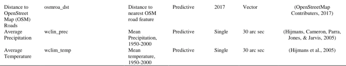
example, we have also tested the model using a minimal set of globally available predictive covariates to provide input to other modelling efforts and avoid circular inference by end users. In the case presented here, chosen covariates were either time-specific or assumed to be temporally invariant (Table 1). All covariates were pre-processed, resampled to 3 arc second (~100m at the Equator) based on data type, and co-registered. All data used to restrict the area of modelling and inform the redistribution of transitions are also detailed in Table 1. Further details on pre-processing of specific covariates are provided in the Supplemental Material.
Table 1. Covariates used for predicting the probability of transition or in the model’s transition re-distribution
process.
Covariate
Variable Name(s) in Random
Forest Description Use Time
Point(s) Original Spatial Resolution(s) Data Source(s) Built-settlement esa_cls190 Binary BS extents Predictive, Restrictive, Redistributive 2000 2005 2010 2015 ESA 10 arc sec (ESA CCI, 2017) DTE Built-settlement
esa_cls190_dst_<year> Distance to the nearest BS edge Predictive 2000 2005 2010 2015 ESA 10 arc sec (ESA CCI, 2017) Proportion Built-settlement 1,5,10,15 esa_cls190_prp_<radius>_<year> Proportion of pixels that are BS within 1,5,10, or 15 pixel radius Predictive 2000 2005 2010 2015 ESA 10 arc sec (ESA CCI, 2017)
Elevation Topo Elevation of
terrain
Predictive 3 arc seconds (Lehner, Verdin, & Jarvis, 2008) Slope Slope Slope of terrain Predictive 3 arc seconds (Lehner et al., 2008) DTE
Protected Areas Level 1
wdpa_cat1_dst_2015 Distance to the nearest level 1 protected area edge
Predictive 2000, 2012
Vector (U.N. Enviroment Programme World Conservation Monitoring
Centre & IUCN World Commission on Protected
Areas, 2015)
Water --- Areas of water
to restrict areas of model prediction
Restrictive 5 arc second (Lamarche et al., 2017)
Subnational Population --- Annual population by sub-national units Predictive, Redistributive 2000 -2020, annually
Vector (Doxsey-Whitfield et al., 2015) Weighted Lights-at-Night (LAN) ---- Annual lagged and sub-national unit normalised LAN Redistributive 2000-2016, annually 30 arc second (2000-2011) 15 arc second (2012-2016) DMSP (WorldPop, Department of Geography and Geosciences, Département de Géographie, & Center for International Earth Science
Information Network (CIESIN), 2018; Zhang,
Pandey, & Seto, 2016) VIIRS(Earth Observation
Group NOAA National Geophysical Data Center,
2016; WorldPop et al., 2018) Travel Time
50k
tt50k Travel time to
the nearest city centre containing at least 50,000 people
Predictive 2000 30 arc second (Nelson, 2008)
Urban Accessibility 2015
urbanaccessibility_2015 Travel time to the nearest city edge
Predictive 2015 30 arc second (Weiss et al., 2018)
ESA CCI Land Cover (LC) Class a
ccilc_dst<class number>_<year> Distance to nearest edge of individual land cover classes
Predictive 2000 10 arc second (ESA CCI, 2017)
Distance to OpenStreet Map (OSM) Rivers osmriv_dst Distance to nearest OSM river feature
Predictive 2017 Vector (OpenStreetMap Contributers, 2017)
6 Distance to OpenStreet Map (OSM) Roads osmroa_dst Distance to nearest OSM road feature
Predictive 2017 Vector (OpenStreetMap Contributers, 2017) Average Precipitation wclin_prec Mean Precipitation, 1950-2000
Predictive Single 30 arc sec (Hijmans, Cameron, Parra, Jones, & Jarvis, 2005) Average
Temperature
wclim_temp Mean
temperature, 1950-2000
Predictive Single 30 arc sec (Hijmans et al., 2005)
a Some classes were collapsed: 10-30 → 11; 40-120 → 40; 150-153 → 150; 160-180 → 160
2.1.1. Built-Settlement Data
We chose to use the “Urban” thematic class, class 190, from the annual ESA CCI landcover dataset, hereafter ESA, for our study because of its annual coverage from 1992 to 2015, allowing for the exclusion of years in the modelling process for validation of outputs. For our period of interest, 2000 to 2015, the ESA data creates annual 10 arc sec resolution (~300m at Equator) datasets by looking for thematic class changes from a baseline land cover map, produced using MERIS imagery, using 30 arc second (~1 km at the Equator) SPOT VGT imagery (1999-2013) and PROBA-V imagery (2014-2015) (UCL Geomatics, 2017). Starting in 2004, if there are changes detected, then the individual pixels of change detected at 30 arc second are further delineated using 10 arc second MERIS or PROBA-V imagery (UCL Geomatics, 2017). To reduce false detections, changes must be observed over two years or more (UCL Geomatics, 2017). Furthermore, the Global Human Settlement Layer (GHSL) (Pesaresi et al., 2013, 2016) and Global Urban Footprint (GUF) (T Esch et al., 2013) datasets are utilized in defining the extents of the ESA Urban class (UCL Geomatics, 2017). While still undergoing full validation, initial validation efforts estimate the 2015 Urban class user and producer accuracies between 86-88 percent and 51-60 percent, respectively (UCL Geomatics, 2017). We also test and validate a single year from an alpha version of
forthcoming multi-temporal World Settlement Footprint (WSF) dataset, known as WSF Evolution (Thomas Esch et al., 2018), and present the results in the Supplementary Material.
Table 2. Summary of built-settlement transition data by country and period. Areal units here are pixels
(~100m) as that is the unit handled by the model which looks at relative areal changes as opposed to absolute areal changes.
Country Period Initial Non-Built Area (pixels) Observed Transitions Panama 2000-2005 8,901,004 0.03 % 2005-2010 8,898,679 0.09 % 2010-2015 8,890,339 0.75 % Switzerland 2000-2005 6,816,510 1.56 % 2005-2010 6,710,069 0.08 % 2010-2015 6,704,973 0.01 % Uganda 2000-2005 28,231,555 0.07 % 2005-2010 28,210,425 0.04 % 2010-2015 28,200,084 0.04 % Vietnam 2000-2005 40,108,425 0.11 % 2005-2010 40,063,545 0.18 % 2010-2015 39,990,858 0.38 % 2.1.2 Population Data
Annual population estimates from 2000 to 2020 for subnational areas were provided by Center for International Earth Science Information Network (CIESIN) in tabular format with unique IDs corresponding to a globally consistent grid containing the unique subnational
7
unit IDs and harmonized coastlines(Doxsey-Whitfield et al., 2015). Populations and their corresponding areas are based upon the Gridded Population of the World (GPW), version 4 and as such follow the methods detailed in Doxsey-Whitfield et al. (2015) for the
interpolation of population between years of official counts or estimates. 2.2 Built-Settlement Growth Model (BSGM)
2.2.1 Overview
Here we interpolated for every year between a set of timepoints, T = {t0, t1, t2, …, t1}
where t0 is the initial observed timepoint, t1 is the final observed timepoint, and all other times tare points lying between t0 and t1 for which we had observed BS extents. The time between any two observed time points t is referred to as a period, p. Within this study, t0 is 2000, t1 is 2015, and we also have observed time points at 2005 and 2010, however the framework can handle any regularly spaced intra-period time-step if the input data corresponds. Therefore, in this study, for the ESA informed models we are carrying out modelling on three time periods, 2000-2005, 2005-2010, 2010-2015, for a total of 12 years interpolated. We generalize the process to determine the timing and number of transitions for each time step independently for each subnational unit, hereafter unit, as follows:
1. Create a population map for all tobserved in T.
2. At all tobserved, for each unit, extract the time-specific population count within the time
specific BS extents and derive the corresponding average BS population density. 3. On a unit-by-unit basis, interpolate the extracted BS population count between each
tobserved using piecewise-fit logistic growth curves and BS population density by fitting
natural cubic splines across all tobserved.
4. Estimate expected unit, time-step-specific, total BS extent area, in number of pixels, and the expected number of transitions for that time-step based upon predicted unit-specific total BS population and BS population density.
5. For every unit, adjust the expected transitions by the sum of all expected transitions across the given period, ta and tb, e.g. 2000-2005 or 2005-2010, and divide by the total
observed changes, e.g. 2005 BS extents minus 2000 BS extents. Repeat for all periods.
6. For each unit, use the adjusted predicted transitions from step five as relative weights within a given unit to dasymetrically redistribute observed transitions from the larger source period to smaller individual time-steps, i.e. years, while maintaining the
original number of transitions when all time-steps are summed. Repeat for all periods. To spatially disaggregate the predicted transitions, we first train a Random Forest (RF) model (Breiman, 2001) to produce a continuous surface representing the probability of a given grid pixel transitioning from non-BS to BS between t0 and t1. For every time-step, processing each subnational unit independently, we utilized unit normalized lagged lights-at-night (LAN) data to annually adjust the base RF-derived transition probabilities. The
assumption behind this being that areas that underwent the largest increase in brightness, relative to the rest of the unit in a single time-step, have a higher probability of transitioning and vice versa. From the pixels that were known to have transitioned, as indicated in the input
8
BS data, we selected pixels with the nth highest probabilities for transition, where n was equal
to the number of pixels predicted to transition for that time-step. We then converted those pixels to BS, recorded the new BS extents, and used those extents as the basis for the next time-step of transitions. This resulted in a series of regularly spaced time-specific binary spatial predictions of the BS extents in raster format. A full process diagram is shown in Figure 1. All modelling and analyses were carried out using R 3.4.2 (R Core Team, 2016) on the IRIDIS 4 high-performance computing cluster (see Supplemental Material for code).
Figure 1. Overview of the generalized modelling process for a case of only two observed timepoints, t0 and t1,
with references to utilized equations.
2.2.2 Random Forest (RF) Estimation of the Probability of Transition
Given that the binary dataset of transition/non-transition constitutes an intrinsic "imbalanced set" (He & Garcia, 2009), i.e. there are many more non-transitions than transitions; we adopted a stratified random over/under-sampling method (He & Garcia, 2009), similar to (Linard et al., 2013), as follows: (i) randomly sample 80 percent of the pixels that transitioned, up to 50,000 and, (ii) randomly sample an equal number of pixels that did not undergo transition. The choice for equal sampling of each stratum was determined by testing different relative proportions and samples sizes until finding the most consistent and best model results, balancing performance and efficiency.
9
To create a probability of transition surface for the complex and non-linear phenomenon of BS transition, we utilized a RF model to accurately and efficiently model across an entire country at the pixel (3 arc second) level in an automatable and parallelizable fashion. We trained the classification RF on whether a pixel had transitioned between time t0 and t1 (1) or not transitioned (0) against the corresponding values of covariates at time t0. We used the constructed RF to predict for the entire given country. Rather than accepting the default output of the RF classifier, which outputs a single predicted class as indicated by the majority of the predictions of its individual constituent trees, we wanted a continuous, 0.00 to 1.00, probability of transitioning in to discriminate between high and low probabilities. Given that we trained the RF as a binary classifier, we took the mean of the individual tree
predictions for each pixel. This class probability has a value between 0.00 and 1.00 represents the posterior probability of a pixel being classified by the RF as transitioning between t0 and
t1 (Breiman, 2001).
2.2.3 Population Mapping of Endpoints
To interpolate, we first needed a spatially-explicit best estimate of the subnational unit specific BS population at all observed timepoints in the modelling period. To get this we created a population surface using the available time-specific and, assumed, time-invariant covariates (see Supplemental Material, Table A2) using the WorldPop RF method, described in Gaughan et al. (Gaughan, Stevens, Linard, Jia, & Tatem, 2013) and Stevens et al. (Stevens, Gaughan, Linard, & Tatem, 2015), to dasymetrically redistribute the time-specific population totals from the subnational unit level to 3 arc second grid pixels (Mennis, 2003; Mennis & Hultgren, 2006; 2015).
For any given time point in the population modelling, we included the distance to nearest BS edge for the t0 timepoint, i.e. 2000, as population relates to older parts of a BS agglomeration differently from newer ones (2016). For example, if we were to model the population map of 2010 we would include the distance to nearest BS edge for 2010 as one of the predictive covariates as well as the distance to nearest BS edge corresponding to the 2000 BS extents. This was done to avoid centres of agglomerations being assigned artificially low population densities relative to the preceding modelled time point (2016). We then extracted and summed by unit the total populations that were spatially coincident with the BS extents and derived the corresponding BS population density for use in the BSGM predictive phases.
2.2.4 Transition Magnitude Estimation
To estimate the number of transitions for each time-step within the study period, we used the predicted BS population changes and the predicted changes in BS population density for every unit. We first interpolated the BS population count of each unit i for every year, BSPOP(t), by fitting logistic growth curves (Booth, 2006), in a piecewise manner, i.e. for each time-period between observed points, using the year-specific total population, Ki(t), as
the varying carrying capacity (Meyer & Ausubel, 1999) as shown in Equation 1 𝐵𝑆𝑃𝑂𝑃𝑖(𝑡) = 𝐾𝑖(𝑡) ∗ 𝑒𝑟𝑖∗𝑡+𝐶𝑖
1+𝑒𝑟𝑖∗𝑡+𝐶𝑖 [Eq. 1]
where t is the number of time steps from the given period’s origin, e.g. for period 2000-2005 2002 corresponds to t = 2, and ri and Ci are determined by fitting a least-squares linear
10
regression to the set of observed values after having been transformed via Equation 2.
ln ( 𝐵𝑆𝑃𝑂𝑃 𝑖𝑡𝑜𝑏𝑠𝑒𝑟𝑣𝑒𝑑
𝐾𝑖𝑡𝑜𝑏𝑠𝑒𝑟𝑣𝑒𝑑−𝐵𝑆𝑃𝑂𝑃𝑖𝑡𝑜𝑏𝑠𝑒𝑟𝑣𝑒𝑑) [Eq. 2]
We then interpolated the unit average BS population density across all observed time points in the study period using natural cubic splines (McNeil, Trussell, & Turner, 1977) and the observed points as the knots, i.e. for ESA 2000, 2005, 2010, and 2015. The overriding theory behind selecting logistic growth curves and the cubic splines for interpolating comes from the sigmoid shape of these curves. That is, BS population and population density are assumed to follow the s-shaped curve by having low growth/decay rate in the beginning, a period of rapid change after a certain point, and then a slowing growth/decay rate as various constraints or carrying capacities, e.g. demographic, environmental, economic, affect the population (J. E. Cohen, 1995; Sibly, 2005).
Using the interpolated unit BS population and the interpolated unit-average BS
population density, we simply relate population and population density to produce areal units, in our case pixels, to get the expected number of transitions in Equation 3
𝐵𝑆𝐶𝑁𝑇𝑖(𝑡) =𝐵𝑆𝑃𝑂𝑃𝑖(𝑡)
𝐵𝑆𝐷𝑖(𝑡) [Eq. 3]
where BSDi(t) is the unit, i, average BS population density at time t. See Supplemental
Materials for how predicted “negative growth” resulting from Equations 1-3 was handled.
2.2.5Dasymetric Redistribution of Transitions Across Time
The number of predicted transitions derived from Equations 1-3 are not inherently constrained by the observed transitions between any two observed time points. To match the total number of observed transitions for the modelled period, we reweighted the transitions of each time-step on a unit-by-unit basis. This is essentially a temporal dasymetric redistribution of transitions from the larger source period, e.g. 2000-2005, to the smaller target periods of t, e.g. 2001,2002, etc., based upon temporal information contained in the time-specific unit population totals. To calculate the weight for each time-step, wt, we write the calculation in
Equation 4 as:
𝑤𝑡𝑖 = 𝐵𝑆𝐶𝑁𝑇̂ (𝑡)𝑖
∑ 𝐵𝑆𝐶𝑁𝑇𝑘1 ̂ (𝑡)𝑖 [Eq. 4]
where t is again relative to the given period from 1 to the last year k and all wt for a given unit
i sum to one. To obtain the temporally weighted transitions, 𝐵𝑆𝐶𝑁𝑇̂ , we multiplied the 𝑖𝑡
weight of each year by the observed number of transitions in Equation 5, rounding to the nearest whole number for each year (see Supplemental Materials, section A4 for obtaining agreement with rounding differences).
11
𝐵𝑆𝐶𝑁𝑇̂ 𝑡𝑖= 𝑟𝑜𝑢𝑛𝑑(𝑤𝑡𝑖∗ ∆𝐵𝑆𝐶𝑁𝑇𝑖) [Eq. 5]
Where ∆𝐵𝑆𝐶𝑁𝑇𝑖 is the number of observed transitions, in pixels, from non-BS to BS for a given unit i. This allows the model to maintain agreement of transitions between the points that we interpolated.
2.2.6 Spatially Disaggregating Transitions Using Annual Unit-specific LAN-weights
For each period, we then processed the tabular predicted transitions into time-specific BS extent maps, i.e. spatially allocated the transitions within each subnational unit for each time-step. We spatially assigned the transitions within each unit using the RF-derived transition probability surface adjusted by time-specific weights in the form of subnational unit normalized LAN brightness differences, i.e. one time-step lags (see Supplemental Material). Given that the non-BS to BS, or “BS growth,” transition process is iterative in nature, we began by taking the extents of the previous time-step, or the previous observed extents if t was equal to one. We limited the location(s) where transitions could be allocated within the subnational unit to pixels where transitions were observed to have occurred, as defined by the input BS data. For every one of those locations, j, assuming they weren't transitioned in previous steps, we retrieved the transition probability as calculated in the transition probability surface. We took this base probability of transition for every pixel j and adjusted it by the spatially coincident lagged and weighted LAN data, for time-step t, using Equation 6:
𝑃𝑎𝑑𝑗(𝑡𝑟𝑎𝑛𝑠𝑖𝑡𝑖𝑜𝑛)𝑖𝑗𝑡 = 𝑤𝐿𝐴𝑁𝑖𝑗𝑡∗ 𝑃(𝑡𝑟𝑎𝑛𝑠𝑖𝑡𝑖𝑜𝑛)𝑖𝑗 [Eq. 6]
where 𝑃(𝑡𝑟𝑎𝑛𝑠𝑖𝑡𝑖𝑜𝑛)𝑖𝑗 is the RF-derived transition probability where transition was
observed, 𝑤𝐿𝐴𝑁𝑖𝑗𝑡 is the corresponding adjusted LAN difference observed for the time-step
t, and 𝑃𝑎𝑑𝑗(𝑡𝑟𝑎𝑛𝑠𝑖𝑡𝑖𝑜𝑛)𝑖𝑗𝑡 is the adjusted probability of transition for the time-step t in a given pixel j within the administrative unit i. Similar to previous models(Linard et al., 2013; Tayyebi et al., 2013), we assumed pixels with a higher probability of transition are more likely to transition before pixels with lower probabilities. We selected the nth highest probabilities from the subset of potential transition pixels, where n was equal to 𝐵𝑆𝐶𝑁𝑇̂ , 𝑡𝑖 changed the value of those selected pixels to represent a transition to BS, and output the union of the new transitions and previous BS extents as the predicted BS extents for that time-step. We repeated this procedure using the newly produced extents for the preceding step as the base BS extent for the next step's transition procedure, until all time-steps for the period were processed and then the entire procedure was repeated until all periods had been processed.
2.3 Analyses
2.3.1 Validation and Comparison Metrics
While the RF produces its own validation estimates (Breiman, 2001), we tested the accuracy of the RF classifier by randomly sampling 100,000 pixels, not utilized in the
12
training of the RF, for validation. We selected this sample size as we were able to obtain sample prevalence rates equal to the known true prevalence rates of each country while still maintaining efficiency. Based on this sample, we plotted receiver operator curves (ROCs) and, given the imbalanced data (Haibo He & Garcia, 2009; Saito & Rehmsmeier, 2015), precision recall curves (PRCs) with simulated perfect and random classifier curves for comparison.
Here, for the ESA models, we are comparing the predicted extents to all withheld extents between 2000 and 2015. For every year of prediction, we determined whether a pixel was True Positive, False Positive, False Negative, or True Negative, TP, FP, FN, TN,
respectively. We calculated contingency table-based metrics to evaluate classification accuracy based primarily on the F1 score (Table 3) which is the harmonic mean of recall and
precision, the quantity disagreement (Pontius & Millones, 2011), and the allocation
disagreement (Pontius & Millones, 2011). We aggregated the pixel level results, to the unit level and calculated the same metrics since precision, and by extension F1, is sensitive to the
corresponding prevalence and is subject to the modifiable areal unit problem (MAUP) (Openshaw, 1984).The MAUP not only reduces variance in value distributions the more the data are aggregated from their original resolution (Openshaw, 1984), but will result in
different prevalences with different subnational area, i.e. zonal, configurations. The equations of the metrics calculated are listed in Table 3.
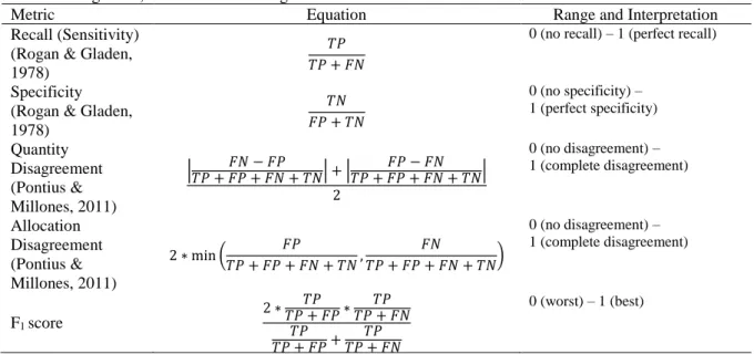
Table 3. Classification agreement metrics utilized and a brief description of each. The F1-score is interpreted as
the harmonic mean of precision and recall. TP is “True Positive”, FP is “False Positive”, FN is “False Negative”, and TN is “True Negative.”
Metric Equation Range and Interpretation Recall (Sensitivity)
(Rogan & Gladen, 1978)
𝑇𝑃 𝑇𝑃 + 𝐹𝑁
0 (no recall) – 1 (perfect recall)
Specificity (Rogan & Gladen, 1978) 𝑇𝑁 𝐹𝑃 + 𝑇𝑁 0 (no specificity) – 1 (perfect specificity) Quantity Disagreement (Pontius & Millones, 2011) |𝑇𝑃 + 𝐹𝑃 + 𝐹𝑁 + 𝑇𝑁𝐹𝑁 − 𝐹𝑃 | + |𝑇𝑃 + 𝐹𝑃 + 𝐹𝑁 + 𝑇𝑁𝐹𝑃 − 𝐹𝑁 | 2 0 (no disagreement) – 1 (complete disagreement) Allocation Disagreement (Pontius & Millones, 2011) 2 ∗ min ( 𝐹𝑃 𝑇𝑃 + 𝐹𝑃 + 𝐹𝑁 + 𝑇𝑁, 𝐹𝑁 𝑇𝑃 + 𝐹𝑃 + 𝐹𝑁 + 𝑇𝑁) 0 (no disagreement) – 1 (complete disagreement) F1 score 2 ∗𝑇𝑃 + 𝐹𝑃𝑇𝑃 ∗𝑇𝑃 + 𝐹𝑁𝑇𝑃 𝑇𝑃 𝑇𝑃 + 𝐹𝑃+𝑇𝑃 + 𝐹𝑁𝑇𝑃 0 (worst) – 1 (best)
Additionally, to assess whether the modelling is worth the effort, we constructed a null model that randomly assigns the transitions to a year within the given period, with every year having an equal likelihood, and carried out predictions for each year within pixels that were known to have transitioned for comparability with our model. Again, we determined for each pixel whether it was a TP, FP, FN, or TN and calculated metrics to compare the BSGM and the null model at the across each country at the pixel level, and at the unit level. The null model
13
was bootstrapped 500 times based upon resource limits and prediction stability, for each year and was specific to each country.
3. RESULTS
Across all study areas, two-thirds of the modelled years correctly predicted between 85-99 percent of transition pixels. For all years, again at the pixel level, the BSGM displayed low quantity and allocation disagreement in both absolute and relative terms. Similarly, the pixel level F1 score, with few exceptions, was higher than the null model, yet had more variance in absolute terms of performance. Comparable results were found at the unit level, with particularly good results in the middle and later years of the study period.
3.1 RF Performance
The ROC plots in Figure 2 show that the RFs approach the performance of the theoretical perfect model. However, given the imbalanced data, the PRC plots (Figure 2) show a more nuanced picture of performance where a maximum level of precision is quickly achieved, remains steady up to a certain value of recall that varies by study area, and then precision quickly decreases with increasing recall.
Figure 2. Receiver Operator Curve (left plots) and Precision Recall Curves (right plots) with the RF model
performance, blue lines, against a random model, red lines, and a perfect model, green lines, for each modelled country and input dataset.
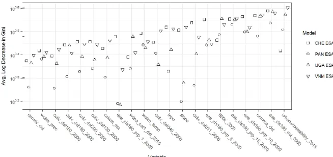
Of the covariates informing the RFs of the models, we consistently saw that the most important predictors of a pixel transitioning from non-BS to BS were covariates related to distance (“esa_cls190_dst_2000”) and local density (“esa_cls190_prp_5_2000”,
“esa_cls190_prp_10_2000”, and “esa_cls190_prp_15_2000”) of BS established at the beginning of the overall study period, i.e. 2000, and connectivity of BS extents at the
14
beginning ("tt50k_2000") or end ("urbanaccessibility_2015" and "osmroa_dst") of the study period (Figure 3).
Figure 3. Random forest covariate importance as measured by the average log decrease in the Gini impurity
when the covariate is used as the splitting criteria at nodes; higher values indicate better performance of covariate. Model for Swizerland (CHE) ESA, Panama (PAN) ESA, Uganda (UGA) ESA, and Vietnam (VNM) ESA, are shown. Refer to Table 1 for covariate names.
3.2 Pixel Level Results
Examining the proportion of pixels known to transition that were predicted correctly in Table 4, we show that out of 49 model years predicted, 33 of those years had correctly predicted proportions between 0.85 and 0.99. The ESA based modelled years ranged from 0.57 to 0.99 of pixels predicted correctly (Table 4). Note that one minus the proportion correct is equal to the total disagreement of the predicted pixels, i.e. the sum of the quantity and allocation disagreement (Pontius & Millones, 2011).
Table 4. Proportion of transition pixels predicted correctly by the BSGM by year. Note that 1 – the proportion
correct is equal to the overall disagreement, i.e. the sum of the quantity and allocation disagreement.
Model 2001 2002 2003 2004 2006 2007 2008 2009 2011 2012 2013 2014 CHE ESA 0.718 0.573 0.628 0.975 0.987 0.979 0.975 0.983 0.999 0.998 0.997 0.997 PAN ESA 0.952 0.935 0.934 0.960 0.806 0.771 0.816 0.920 0.905 0.838 0.801 0.818 UGA ESA 0.814 0.787 0.803 0.929 0.912 0.877 0.877 0.909 0.940 0.893 0.865 0.878 VNM ESA 0.942 0.918 0.923 0.951 0.923 0.872 0.866 0.916 0.879 0.777 0.738 0.790
Examining the year-specific study area F1 scores in Figure 4, we show that the BSGM had low performance between 2001 to 2003, in absolute terms, and relatively near null model performance, across all ESA study areas. The F1 score for all modelled years after 2003 increases to quite good performance, with values approaching 1.0 in some cases, and the difference between the BSGM and null model performance increases even more dramatically (Figure 4).
15
Figure 4. Pixel-level F1 score by year for Switzerland (CHE), Panama (PAN), Uganda (UGA), and Vietnam
(VNM) as compared to a null model. Full annual contingency data and metrics in supplementary material
Examining the source of the disagreement further, we display the observed quantity and allocation disagreement as well as the corresponding disagreements under the null model in Figure 5. We show that for all modelled years using the ESA data, the total disagreement is substantially less than that of the null model and predominantly, the disagreement produced by the BSGM model is predominantly due to allocation error (Figure 5). However, there does appear to be a pattern of increasing disagreement due to quantity error after 2010.
Figure 5. Pixel-level quantity and allocation disagreement of BSGM and null models for Switzerland (CHE),
Panama (PAN), Uganda (UGA), and Vietnam (VNM) as compared to a null model, given in red. Full annual contingency data and metrics in supplementary material
16
3.3 Subnational Unit Level Results
Overall, at the unit level, we found results similar to the pixel-level results, including poor performance in absolute terms between 2001 to 2003, but some units were obviously performing worse than others as compared to the null model. Plotting the ESA-informed model distributions of unit-level F1 scores by study area and year against the corresponding null model performance, we show that the BSGM generally performs better in the majority of subnational units from which the transitions were disaggregated from (Figure 6). At worst, e.g. Vietnam 2002, approximately half of the units were still performing better than the null model (Figure 6). For quantity disagreement (Figure 7) and allocation disagreement (Figure 8), results similar to pixel level results were found.
Figure 6. Unit level F1 score box plots, by dasymetric period, of Switzerland (CHE), Panama (PAN), Uganda
(UGA), and Vietnam (VNM) ESA informed models as compared to a null model, given by a red “x”. Number of units exhibiting any transitions for each period and a defined metric value is given above the x-axis.
17
Figure 7. Unit level quantity disagreement box plots, by dasymetric period, of Switzerland (CHE), Panama
(PAN), Uganda (UGA), and Vietnam (VNM) ESA informed models as compared to a null model, given by a red “x”. Number of units exhibiting any transitions for each period and a defined metric value is given above the x-axis.
Figure 8. Unit level allocation disagreement box plots, by dasymetric period, of Switzerland (CHE), Panama
(PAN), Uganda (UGA), and Vietnam (VNM) ESA informed models as compared to a null model, given by a red “x”. Number of units exhibiting any transitions for each period and a defined metric value is given above the x-axis.
Plotting the unit-level metrics for all models as choropleth maps (see Supplementary Material for select maps and shape files containing contingency data), shows that years of generally good performance, the units of lesser performance are those that correspond to areas of less densely settled areas and the peripheries of established urban areas. Other years,
18
such as Uganda 2001, performed poorly across many units with no apparent pattern. Identical analyses for the WSF Evolution data are given in the supplementary materials as well.
4. DISCUSSION
The 2030 SDGs, have reinforced the importance of data to being able to account for “all people everywhere (United Nations, 2016). Differences in the dynamic spatial distributions of hazards (Carrão, Naumann, & Barbosa, 2016; Oliveira, Oehler, San-Miguel-Ayanz, Camia, & Pereira, 2012), the spatial variation of the effects of climate change (Ericson, Vorosmarty, Dingman, Ward, & Meybeck, 2006; Hanjra & Qureshi, 2010; Stephenson et al., 2010), spatially allocating services to ensure sufficient coverage (Eckert & Kohler, 2014; Sverdlik, 2011), and targeting interventions and planning (Linard, Alegana, Noor, Snow, & Tatem, 2010; Utazi et al., 2018) based upon local context with limited resources requires more accurate mapping of BS and mapping of populations, both large and small (United Nations, 2016). Here we have shown a flexible modelling framework constructed from open-source methods and covariates to produce a framework that can be scaled to global extent across a variety of study areas and input data. This model approximates patterns of BS growth through time with good agreement for most years at the pixel and the units used in disaggregation (Table 4, Figures 4 and 6). Here we have shown the BSGM framework is capable of filling gaps of imagery-derived urban feature datasets by estimating the extents in between observations. This emphasizes the strength of using an interpolative model, such as BSGM, as opposed to more imagery dependent annual feature extraction methods that may encounter adverse atmospheric conditions, limited sensor revisits, or the need for more resource intensive imagery-based interpolation methods. This framework, and resultant output data, can be used for better modelling of population through time, inform future urban feature extraction from imagery, help facilitate intervention/planning/monitoring of
development goals, and potentially serve as a platform for simulating different transition paths through time and investigating correlates of BS spatial growth.
However, the BSGM is neither without error not a total replacement for urban feature extractions. Given that the BSGM is interpolative, its predictions are limited by the accuracy, the spatial quality, and the temporal quality of its input urban feature dataset, the input time-specific subnational population data, and the input population surfaces. For
example, the poorer model performance seen from 2001 through 2003 (Figures 4-8) are likely due to the fact the ESA data did not delineate changes, detected at 30 arc sec resolution, at 10 arc second resolution due to the MERIS and PROBA V imagery not being available (UCL Geomatics, 2017). With regards to total disagreement of the model (Figure 5), the relatively high contribution of allocation disagreement prior to circa 2010 and corresponding decrease in contribution post-2010 is likely due to the switch from using coarser DMSP-based LAN data to VIIRS-based LAN data at the 2012 time point.
Further, models are limited by their conceptual and mathematical assumptions. In this framework, we are assuming a certain relationship between relative population and
population density changes and drive demand for temporally coincident settlement growth. This is not to say the assumed relationship is correct; here we assume BS population grows logistically with a time varying capacity that is temporally coincident, i.e. not lagged, and we assume BS population density follows a natural cubic spline across all observed points. This
19
is further predicated upon the assumption that the BS growth is predominantly driven by changes in population and or population density and the resulting demand is instantaneously filled as opposed to being delayed temporally. While there is support for population change being an empirical and theoretical driver of urban/BS growth (Angel et al., 2011; Dyson, 2011; Linard et al., 2013; Seto et al., 2011, 2012), there is also evidence for the use of other covariates, not used here because of their unavailability at subnational levels globally through time, such as Gross Domestic Product and arable land per capita (Angel et al., 2011; Seto et al., 2011). Furthermore, there are other “intangibles” such as local, regional, and national land use or development policies, which almost certainly shape BS growth, but are typically not in an accessible format, if available at all. The value of using population data to predict growth of settlement, shown here in a semi-independent model framework, and the value of using urban/settlement feature data sets to predict population distribution (Nieves et al., 2017), raises the question of whether it is worthwhile or proper to try to fully separate population and settlement given their reciprocal causal links, i.e. population begets built environment and settlement, settlement, typically, begets more population.
The modelling assumptions here are preceded by the assumption of exponential
interpolation of annual population totals by the GPWv4-based data (Doxsey-Whitfield et al., 2015) and that the RF-informed dasymetric redistribution of those population totals are correctly locating the population in a manner which leads to correct BS population estimates for the BSGM to utilize. We already know that the RF population model tends to
underestimate populations in BS and overestimate populations outside of urbanized areas (Stevens et al., 2015). Since the BSGM allocates transitions based upon relative changes in BS population, this last point should not affect prediction timings, assuming the RF-informed population modelling biases are consistent between the two times. Alternatively, any spatially explicit population datasets can be used as inputs for the BSGM, even the base GPW4,
removing the need to use a modelled population input. With any area-based metric the
Modifiable Areal Unit Problem (Openshaw, 1984) must be considered, as the total number of pixels in each unit is typically larger in the less settled areas resulting in less variation of aggregated metric values in those areas. With dasymetric redistribution methods, the size and configuration of the source units, spatially or temporally, can also affect the quality of the disaggregation with the larger relative differences between source unit and target unit sizes introducing more uncertainty to the output (Mennis, 2003; Mennis & Hultgren, 2006). As the concept of urban growth can be thought of as an incremental process, with future outcome dependent upon previous growth, the gridded outputs of the BSGM can be aggregated across years to decrease uncertainty of the interpolated extents should annual datasets not be needed.
5. CONCLUSIONS
As urban feature dataset producers such as ESA, MAUPP, GHSL, GUF and others continue to improve and release datasets with higher temporal resolution, models such as the BSGM will likely still have utility due to imagery/extraction issues and a need to smooth or fill-in time periods where difficulty was experienced (ESA CCI, 2017; T Esch et al., 2013; Forget, Linard, & Gilbert, 2018; Pesaresi et al., 2016). By the time annual urban feature extractions have filled the current demand and become the standard, there will have grown a demand for quarterly, monthly, and so on, feature extractions and an interpolative model will
20
attempt to fill the need, data permitting, until the imagery and computational resources can. This is not to say that interpolative models and imagery-extracted features are oppositional, but rather are complementary. Should the time come where high-resolution annual feature datasets become the norm, this would offer a wealth of information from which to improve the model assumptions the BSGM currently makes. Further, the predictions of the BSGM could serve as a comparative check in the production of future urban feature extractions and a platform to explore population and BS dynamics.
As informative as urban feature extraction datasets are, imagery will never see into the future and we plan on extending this framework to allow for projection of BS growth, both in a predictive manner as well as allowing scenarios to be input. We found that the primary predictors of growth BS extents were related to connectivity, i.e. road networks, and local, i.e. ~0.5-1.5km, settlement density (Figure 3) both giving support to work in attempting to define “urban” base on contiguity, connectivity, and spatial density (Dijkstra & Poelman, 2014; T Esch et al., 2014; Pesaresi & Freire, 2016) and implying that investment in
detecting/simulating new road network data would be beneficial to better predicting urban feature extents. Still mostly unknown is how the BSGM would perform for smaller
settlements, not captured by coarser datasets such as the ESA land cover, and we are looking to test this with forthcoming feature data sets with resolutions below 3 arc seconds. Lastly, we plan to validate the utility of these dataset in an applied manner by comparing the effects of including the BSGM derived extents in annual population modelling.
Here we have presented an open source framework for interpolating a binary BS or urban feature dataset using a limited covariate dataset that can be used to further population mapping by filling a current gap in annual global urban feature datasets. This framework is scalable globally, but also allows for sub-study area variation in transition probability, population changes, and lights-at-night changes to drive the overall study area model.
Further, the model can be adapted to run at other scales, both spatially and temporally, either by modifying the provided code or in many cases, simply by modifying the input data. The annual global interpolative and projected datasets from 2000 to 2020, produced with an early version of this model with a reduced covariate set, is freely available on the WorldPop website (worldpop.org) with the up to date model production code hosted on the WorldPop GitHub repository (github.com/wpgp/BSGMi_alpha). The specific model code used in producing this work is included in the supplementary material.
21
REFERENCES
Angel, S., Parent, J., Civco, D. L., Blei, A. M., & Potere, D. (2011). The Dimensions of Global Urban Expansion: Estimates and Projections for All Countries, 2000-2050.
Progress in Planning, 75, 53–107. https://doi.org/10.1016/j.progress.2011.04.001
Angel, S., Sheppard, S. C., & Civco, D. L. (2005). The Dynamics of Global Urban
Expansion. Washington, D. C.: The World Bank.
Barredo, J. I., Demicheli, L., Lavalle, C., Kasanko, M., & McCormick, N. (2004). Modelling Future Urban Scenarios in Developing Countries: An Application Case Study in Lagos, Nigeria. Environment and Planning B, 31, 65–84.
Bartholomé, E., & Belward, A. S. (2005). GLC2000: a new approach to global land cover mapping from Earth observation data. International Journal of Remote Sensing, 26(9), 1959–1977. https://doi.org/10.1080/01431160412331291297
Batty, M. (2009). Urban Modeling. In International Encyclopedia of Human Geography (pp. 51–58). Oxford, UK: Elsevier.
Batty, M., & Xie, Y. (1994). From Cells to Cities. Environment and Planning B, 21, S31– S48.
Booth, H. (2006). Demographic forecasting: 1980 to 2005 in review. International Journal of
Forecasting, 22(3), 547–581. https://doi.org/10.1016/j.ijforecast.2006.04.001
Breiman, L. (2001). Random Forests. Machine Learning, 45(1), 5–32.
Carrão, H., Naumann, G., & Barbosa, P. (2016). Mapping global patterns of drought risk: An empirical framework based on sub-national estimates of hazard, exposure and
vulnerability. Global Environmental Change, 39, 108–124. https://doi.org/10.1016/j.gloenvcha.2016.04.012
Chongsuvivatwong, V., Phua, K. H., Yap, M. T., Pocock, N. S., Hashim, J. H., Chhem, R., … Lopez, A. D. (2011). Health and health-care systems in southeast Asia: diversity and transitions. The Lancet, 377(9763), 429–437.
https://doi.org/10.1016/S0140-6736(10)61507-3
Clarke, K. C., & Gaydos, L. (1998). Loose-coupling a Cellular Automaton Model and GIS: Long-term Urban Growth Prediction for San Francisco and Washington/Baltimore.
International Journal of Geographic Information Sciences, 12(7), 699–714.
Clarke, K. C., Hoppen, S., & Gaydos, L. (1997). A Self-modifying Cellular Automaton Model of Historical Urbanization in the San Francisco Bay Area. Environment and
Planning B, 24, 247–261.
Cohen, B. (2006). Urbanization in Developing Countries: Current Trends, Future Projections, and Key Challenges for Sustainability. Technology in Society, 28, 63–80.
Cohen, J. E. (1995). Population Growth and Earth’s Human Carrying Capacity. Science,
269(5222), 341–346.
Dhingra, M. S., Artois, J., Robinson, T. P., Linard, C., Chaiban, C., Xenarios, I., … Gilbert, M. (2016). Global mapping of highly pathogenic avian influenza H5N1 and H5Nx clade 2.3.4.4 viruses with spatial cross-validation. ELife, 5.
https://doi.org/10.7554/eLife.19571
Dijkstra, L., & Poelman, H. (2014). A harmonized definition of cities and rural areas: the
new degree of urbanization (Regional Working Paper No. WP 01/2014). Retrieved from
http://ec.europa.eu/regional_policy/sources/docgener/work/2014_01_new_urban.pdf Doxsey-Whitfield, E., MacManus, K., Adamo, S. B., Pistolesi, L., Squires, J., Borkovska, O.,
& Baptista, S. R. (2015). Taking advantage of the improved availability of census data: A first look at the Gridded Population of the World, Version 4. Papers in Applied
Geography, 1(3), 226–234. https://doi.org/10.1080/23754931.2015.1014272
Dyson, T. (2011). The role of the demographic transition in the process of urbanization.
22
Earth Observation Group NOAA National Geophysical Data Center. (2016). VIIRS
Nighttime Lights - One Month Composites. Boulder, Colorado: NOAA National Centers for Environmental Information. Retrieved from
https://ngdc.noaa.gov/eog/viirs/download_dnb_composites.html
Eckert, S., & Kohler, S. (2014). Urbanization and Health in Developing Countries: A Systematic Review. World Health & Population, 15(1), 7–20.
Ericson, J. P., Vorosmarty, C. J., Dingman, S. L., Ward, L. G., & Meybeck, M. (2006). Effective sea-level rise and deltas: Causes of change and human dimension implications.
Global and Planetary Change, 50, 63–82.
ESA CCI. (2017). European Space Agency Climate Change Initiative Landcover. European Space Agency. Retrieved from http://maps.elie.ucl.ac.be/CCI/viewer/download.php Esch, T., Bachofer, F., Heldens, W., Hirner, A., Marconcini, M., Palacios-Lopez, D., …
Gorelick, N. (2018). Where We Live—A Summary of the Achievements and Planned Evolution of the Global Urban Footprint. Remote Sensing, 10(6), 895.
https://doi.org/10.3390/rs10060895
Esch, T., Marconcini, M., Felbier, A., Roth, A., Heldens, W., Huber, M., … Dech, S. (2013). Urban Footprint Processor - Fully Automated Processing Chain Generating Settlement Masks from Global Data of the TanDEM-X Mission. IEEE Geoscience and Remote
Sensing Letters, 10(6), 1617–1621.
Esch, T., Marconcini, M., Marmanis, D., Zeidler, J., Elsayed, S., Metz, A., & Dech, S. (2014). Dimensioning urbanization - An advanced procedure for characterizing human settlement properties using spatial network analysis. Applied Geography, 55, 212–228. https://doi.org//j.apgeog.2014.09.009
Forget, Y., Linard, C., & Gilbert, M. (2018). Supervised Classification of Built-Up Areas in Sub-Saharan African Cities Using Landsat Imagery and OpenStreetMap. Remote
Sensing, 10(7), 1145. https://doi.org/10.3390/rs10071145
Gaughan, A. E., Stevens, F. R., Huang, Z., Nieves, J. J., Sorichetta, A., Lai, S., … Tatem, A. J. (2016). Spatiotemporal Patterns of Population in Mainland China, 1990 to 2010.
Scientific Data, 3, 160005. https://doi.org/10.1038/sdata.2016.5
Gaughan, A. E., Stevens, F. R., Linard, C., Jia, P., & Tatem, A. J. (2013). High Resolution Population Distribution Maps for Southeast Asia in 2010 and 2015. PLoS One, 8(2), e55882. https://doi.org/10.1371/journal.pone.0055882
Goldewijk, K. K., Beusen, A., & Janssen, P. (2010). Long-term dynamic modeling of global population and built-up area in a spatially explicit way: HYDE 3.1. The Holocene,
20(4), 565–573. https://doi.org/10.1177/0959683609356587
Haibo He, & Garcia, E. A. (2009). Learning from Imbalanced Data. IEEE Transactions on
Knowledge and Data Engineering, 21(9), 1263–1284.
https://doi.org/10.1109/TKDE.2008.239
Hanjra, M. A., & Qureshi, M. E. (2010). Global Water Crisis and Future Food Security in an Era of Climate Change. Food Policy, 35, 365–377.
https://doi.org/10.1016/j.foodpol.2010.05.006
He, H., & Garcia, E. A. (2009). Learning from Imbalanced Data, 21(9), 1263–1284. Hijmans, R. J., Cameron, S. E., Parra, J. L., Jones, P. G., & Jarvis, A. (2005). Very high
resolution interpolated climate surfaces for global land areas. International Journal of
Climatology, 25, 1965–1978.
Lamarche, C., Santoro, M., Bontemps, S., D’Andrimont, R., Radoux, J., Giustarini, L., … Arino, O. (2017). Compilation and Validation of SAR and Optical Data Products for a Complete and Global Map of Inland/Ocean Water Tailored to the Climate Modeling Community. Remote Sensing, 9(36). https://doi.org/10.3390/rs9010036
23
Region Using a Cellular Automata-based Model. Journal of Urban Planning and
Development, 130(3), 145–158.
Lehner, B., Verdin, K., & Jarvis, A. (2008). New Global Hydrography Derived from Spaceborne Elevation Data. Eos, Transactions of the American Geophysical Union,
89(10), 93–94. https://doi.org/10.1029/2008EO100001
Linard, C., Alegana, V., Noor, A. M., Snow, R. W., & Tatem, A. J. (2010). A high resolution spatial population database of somolia for disease risk mapping. International Journal of
Health Geographics, 9(1), 45.
Linard, C., Tatem, A. J., & Gilbert, M. (2013). Modelling Spatial Patterns of Urban Growth in Africa. Applied Geography, 44, 23–32.
McGranahan, G., Balk, D., & Anderson, B. (2007). The Rising Tide: Assessing the Risks of Climate Change and Human Settlements in Low Elevation Coastal Zones. Environment
& Urbanization, 19(1), 17–37. https://doi.org/10.1177/0956247807076960
McNeil, D. R., Trussell, T. J., & Turner, J. C. (1977). Spline Interpolation of Demographic Data. Demography, 14(2), 245–252. Retrieved from
https://www.jstor.org/stable/2060581
Mennis, J. (2003). Generating surface models of population using dasymetric mapping.
Professional Geographer, 55(1), 31–42.
Mennis, J., & Hultgren, T. (2006). Intelligent dasymetric mapping and its application to areal interpolation. Cartography and Geographic Information Science2, 33, 179–194.
Meyer, P. S., & Ausubel, J. H. (1999). Carrying capacity: A model with logistically varying limits. Technological Forecasting and Social Change, 61(3), 209–214.
https://doi.org/10.1016/S0040-1625(99)00022-0
Nelson, A. (2008). Estimated Travel Time to the Nearest city of 50,000 or More People in Year 2000. Ispra, Italy: Global Environment Monitoring Unit - Joint Research Centre of the European Commission. Retrieved from
http://forobs.jrc.ec.europa.eu/products/gam/sources.php
Nieves, J. J., Stevens, F. R., Gaughan, A. E., Linard, C., Sorichetta, A., Hornby, G., … Tatem, A. J. (2017). Examining the correlates and drivers of human population distributions across low- and middle-income countries. Journal of The Royal Society
Interface, 14(137), 20170401. https://doi.org/10.1098/rsif.2017.0401
Oliveira, S., Oehler, F., San-Miguel-Ayanz, J., Camia, A., & Pereira, J. M. C. (2012). Modeling spatial patterns of fire occurrence in Mediterranean Europe using Multiple Regression and Random Forest. Forest Ecology and Management, 275(July 2012), 117– 129. https://doi.org/10.1016/j.foreco.2012.03.003
Openshaw, S. (1984). The modifiable areal unit problem. Concepts and Techniques in
Modern Geography, 38.
OpenStreetMap Contributers. (2017). OpenStreetMap (OSM) Database. OSM. Retrieved from openstreetmap.org
Patel, N., Angiuli, E., Gamba, P., Gaughan, A. E., Lisini, G., Stevens, F. R., … Trianni, G. (2015). Multitemporal Settlement and Population Mapping From Landsat Using Google Earth Engine. International Journal of Applied Earth Observation and Geoinformation,
35(Part B), 199–208. https://doi.org/10.1016/j.jag.2014.09.005
Pesaresi, M., Ehrlich, D., Ferri, S., Florczyk, A. J., Freire, S., Halkia, S., … Syrris, V. (2016).
Operating Procedure for the Production of the Global Human Settlement Layer from Landsat Data of the Epochs 1975, 1990, 2000, and 2014. Publications Office of the
European Union. Retrieved from doi: 10.2788/253582
Pesaresi, M., & Freire, S. (2016). GHS settlement grid, following the REGIO model 2014 in application to GHSL Landsat and CIESIN GPW v4-multitemporal (1975-1990-2000-2015). Retrieved October 26, 2018, from
http://data.jrc.ec.europa.eu/dataset/jrc-ghsl-24 ghs_smod_pop_globe_r2016a
Pesaresi, M., Guo, H., Blaes, X., Ehrlich, D., Ferri, S., Gueguen, L., … Zanchetta, L. (2013). A Global Human Settlement Layer from Optical HR/VHR Remote Sensing Data: Concept and First Results. IEEE Journal of Selected Topics in Applied Earth
Observation & Remote Sensing, 6(5), 2102–2131.
https://doi.org/10.1109/JSTARS.2013.2271445
Pontius, R. G., & Millones, M. (2011). Death to Kappa: birth of quantity disagreement and allocation disagreement for accuracy assessment. International Journal of Remote
Sensing, 32(15), 4407–4429. https://doi.org/10.1080/01431161.2011.552923
Potere, D., & Schneider, A. (2007). A critical look at representations of urban areas in global maps. GeoJournal, 69(1–2), 55–80. https://doi.org/10.1007/s10708-007-9102-z
Potere, D., Schneider, A., Angel, S., & Civco, D. (2009). Mapping urban areas on a global scale: which of the eight maps now available is more accurate? International Journal of
Remote Sensing, 30(24), 6531–6558. https://doi.org/10.1080/01431160903121134
R Core Team. (2016). R: A Language and Environment Layer for Statistical Computing. Vienna, Austria: R Foundation for Statistical Computing. Retrieved from https://www.r-project.org
Rogan, W. J., & Gladen, B. (1978). Estimating prevalence from the results of a screening test. American Journal of Epidemiology, 107(1), 71–76.
Saito, T., & Rehmsmeier, M. (2015). The Precision-Recall Plot is More Informative than the ROC Plot When Evaluating Binary Classifiers on Imbalanced Datasets. PLoS One,
10(3), e0118432. https://doi.org/10.1371/journal.pone.0118432
Sante, I., Garcia, A. M., Miranda, D., & Crecente, R. (2010). Cellular Automata Models for the Simulation of Real-world Urban Processes: A Review and Analysis. Landscape and
Urban Planning, 96, 108–122. https://doi.org/10.1016/j.landurbplan.2010.03.001
Schneider, A., Friedl, M. A., McIver, D. K., & Woodcock, C. E. (2003). Mapping Urban Areas by Fusing Multiple Sources of Coarse Resolution Remotely Sensed Data.
Photogrammetry & Remote Sensing, 69(12), 1377–1386.
Schneider, A., Friedl, M. A., & Potere, D. (2010). Mapping Urban Areas Using MODIS 500-m Data: New Methods and Datasets Based on “Urban Ecoregions.” Re500-mote Sensing of
the Environment, 114, 1733–1746.
Schneider, A., & Woodcock, C. E. (2008). Compact, Dispersed, Fragmented, Extensive? A Comparison of Urban Growth in Twenty-five Global Cities using Remotely Sensed Data, Pattern Metrics and Census Information. Urban Studies, 45(3), 659–692. https://doi.org/10.1177/0042098007087340
Seto, K. C., Fragkias, M., Guneralp, B., & Reilly, M. K. (2011). A Meta-Analysis of Global Urban Land Expansion. PLoS One, 6(8), e23777.
https://doi.org/10.1371/journal.pone.0023777
Seto, K. C., Guneralp, B., & Hutyra, L. R. (2012). Global Forecasts of Urban Expansion to 2030 and Direct Impacts on Biodiversity and Carbon Pools. Proceedings of the National
Academy of Sciences of the United States of America, 109(40), 16083–16088.
https://doi.org/10.1073/pnas.1211658109
Sibly, R. M. (2005). On the Regulation of Populations of Mammals, Birds, Fish, and Insects.
Science, 309(5734), 607–610. https://doi.org/10.1126/science.1110760
Small, C. (2009). The color of cities:An overview of urban spectral diversity. In M. Herold & P. Gamba (Eds.), Global Mapping of Human Settlements (pp. 59–106). New York: Taylor & Francis.
Stephenson, J., Newman, K., & Mayhew, S. (2010). Population dynamics and climate change: What are the links? Journal of Public Health, 32(2), 150–156.