Soft-computing based intelligent adaptive control design of complex dynamic systems

UNIVERSITÉ DU QUÉBEC

THÈSE PRÉSENTÉE À

L’UNIVERSITÉ DU QUÉBEC À TROIS-RIVIÈRES

COMME EXIGENCE PARTIELLE DU DOCTORAT EN GÉNIE ÉLECTRIQUE

PAR

HICHAM CHAOUI

COMMANDE ADAPTATIVE DE SYSTÈMES À DYNAMIQUE COMPLEXE BASÉE SUR L’INTELLIGENCE ARTIFICIELLE

Université du Québec à Trois-Rivières

Service de la bibliothèque

Avertissement

L’auteur de ce mémoire ou de cette thèse a autorisé l’Université du Québec

à Trois-Rivières à diffuser, à des fins non lucratives, une copie de son

mémoire ou de sa thèse.

Cette diffusion n’entraîne pas une renonciation de la part de l’auteur à ses

droits de propriété intellectuelle, incluant le droit d’auteur, sur ce mémoire

ou cette thèse. Notamment, la reproduction ou la publication de la totalité

ou d’une partie importante de ce mémoire ou de cette thèse requiert son

autorisation.

UNIVERSITY OF QUEBEC

THESIS SUBMITTED TO

UNIVERSITÉ DU QUÉBEC À TROIS-RIVIÈRES

IN PARTIAL FULFILLMENT OF THE REQUIREMENTS FOR THE DEGREE OF DOCTOR OF PHILOSOPHY IN ELECTRICAL ENGINEERING

BY

HICHAM CHAOUI

SOFT-COMPUTING BASED INTELLIGENT ADAPTIVE CONTROL DESIGN OF COMPLEX DYNAMIC SYSTEMS

UNIVERSITÉ DU QUÉBEC À TROIS-RIVIÈRES DOCTORAT EN GÉNIE ÉLECTRIQUE (PH.D.)

Programme offert par L’Université du Québec à Trois-Rivières Soft-Computing Based Intelligent Adaptive

Control Design of Complex Dynamic Systems PAR

HICHAM CHAOUI

Pierre Sicard, directeur de recherche Université du Québec à Trois-Rivières

Ahmed Chériti, président du jury Université du Québec à Trois-Rivières

Adel-Omar Dahmane, évaluateur Université du Québec à Trois-Rivières

Philippe Lautier, évaluateur externe Vestas Wind Systems

"Ifwe knew what we were doing it wouldn't be research, would it?"

Albert Einstein. Einstein showed in the early years of the 20th century that time is a relative concept, and hence, it is subjected to change according to the environment (time is dependent on mass and velocity). This fact has been proved with Einstein's theory ofrelativity.

1

~j\~j\ ~\r

In the name of God, Most Gracious, Most Merciful.

"A day with your Lord is equivalent to a thousand years in the way you count"

Sourate Sajda (32), Verse s. 1

~j\~j\~\r

, ~

~

Ji -'

In the name of God, Most Gracious, Most Merciful.

"0 my Lord, advance me in knowledge"

Sourate Tâ-Hâ (20), Verse 114.

Résumé

En dépit des récentes avancées dans le domaine du contrôle des systèmes non-linéaires, les techniques classiques de contrôle dépendent en grande partie sur des modèles mathéma-tiques précis du système à contrôler pour fournir des performances satisfaisantes. En pratique, à cause de non-linéarités élevées, dériver un modèle mathématique décrivant avec précision la dynamique du système à contrôler peut s'avérer une tâche très difficile. Bien que des stratégies de contrôle comme la commande adaptative et le mode de glissement compensent pour les incertitudes paramétriques, ces méthodes sont encore vulnérables en présence d'incertitudes de modélisation, aussi appelées incertitudes non structurées. D'autre part, les contrôleurs à base d'intelligence artificielle n'ont pas une telle lirnitation puisqu'ils ne dépendent pas d'une représentation mathématique du système à contrôler. Malgré les récents résultats, les con-trôleurs à base de réseaux de neurones demeurent incapables d'intégrer de l'expertise sous forme de règles et les contrôleurs à base de la logique floue sont incapables d'incorporer des connaissances déjà acquises sur la dynamique du système.

Basé sur la motivation ci-dessus, cette thèse a pour but de contribuer à l'évolution récente et les mérites de ces outils par le développement de nouvelles structures de commande adap-tative. Les contrôleurs proposés supposent que la dynamique des systèmes est incertaine ou inconnue pour obtenir une robustesse à la fois des incertitudes structurées et non structurées de grandeurs et natures différentes. Les contrôleurs classiques offrent une faible performance en présence de ces sortes d'incertitudes. Contrairement à ces approches, les contrôleurs proposés sont basées sur l'intelligence artificielle, qui n'ont pas de telles limitations, grâce à leur capacité d'apprentissage et de généralisation. Cependant, ces outils sont souvent basés sur des heuris-tiques et le réglage peut ne pas être évident. En outre, de nombreux contrôleurs intelligents soufrent de manque de preuves de stabilité dans les différentes applications de commande. Dans cette thèse, les architectures de contrôle proposées sont conçues en utilisant des tech-niques d'adaptation à base de Lyapunov au lieu des méthodes conventionnelles d'adaptation heuristique. Ainsi, la stabilité est garantie contrairement à beaucoup de systèmes de contrôle basés sur l'intelligence artificielle. Un résumé substantiel est disponible en annexe.

Abstract

Nonlinear dynamical systems face numerous challenges that need to be addressed such as, severe nonlinearities, varying operating conditions, structured and unstructured dynarnical uncertainties, and external disturbances. In spite of the recent advances in the area of nonlin-ear control systems, conventional control techniques depend heavily on precise mathematical system models to provide satisfactory performance. In real life, and due to high nonlinearities, deriving a precise model could be a difficult undertaking. Although convention al nonlinear control strategies, such as adaptive and sliding mode controllers, compensate for parametric uncertainties, they are still vulnerable in the presence of unstructured modeling uncertainties. On the other hand, computational intelligence based controllers do not have su ch a limita-tion, thanks to their mathematical model dependence free characteristic. Despite of the recent results, neural network-based controllers remain incapable of incorporating any human-like expertise and fuzzy logic-based controllers are unable to incorporate any learning already ac-quired about the dynamics of the system in hand.

Driven by the aforementioned motivation, this thesis is meant to contribute to the latest developments and merits of such tools by novel adaptive control methodologies developments. The proposed controllers assume uncertain/unknown systems dynamics to achieve robustness to both structured and unstructured uncertainties of higher and different magnitudes. Conven-tional control structures offer poor performance in the presence of these kinds of uncertainties. Unlike these approaches, the proposed controllers are based on soft-computing tools, which do not have such limitations, thanks to their learning and generalization capabilities. However, these tools are often based on heuristics and tuning may not be trivial. Furthermore, many soft-computing based controllers lack stability proofs in various control applications. In this thesis, the proposed control architectures are designed using Lyapunov-based adaptation techniques instead of conventional heuristic tuning methods. Thus, the stability of the proposed controllers is guaranteed unlike many computational intelligence-based control schemes.

Acknowledgements

First and foremost, words cannot express the gratitude l owe the Lord for his guidance, relief in difficult moments, and success. In fact, if l try to count all His bounties, l won't be able to number them.

l also would like to thank the thesis advisor, Dr. Pierre Sicard, for his support and insight throughout my doctoral studies. Many thanks for being human in the way he treats his students, the way he encourages and respects them. l also feel so grateful for his support during both my master degrees.

l wish to thank the reviewers for their thorough review, very relevant comments and for their suggestions to improve the quality of this thesis.

Special thanks to Dr. Alfred Ng and Dr. James Lee from the Canadian Space Agency (CSA) for their time and support. Thanks for sharing with us the difficulties of spacecraft formation missions, as well as the free-flyer experimental data to validate our approach.

l thank my parents, Mr. Mohamed Chaoui and Mrs. Hania Daoudi, as well as my family members for their support throughout ail my studies. Mom, your dream now becomes true. My parents have made many personal sacrifices to provide me the best possible education, it is impossible ta put words on their contribution.

Finally l would like to thank my wonderful sister, Samira, and my lovely wife, Laurie, for their patience and encouragements over the years.

Thanks to ail those who have contributed to this work.

To aIl engineers working in the field of renewable energy to make our planet greener.

To a11 researchers who love contributing to soft-computing techniques.

To aIl control systems researchers worldwide.

To aIl my friends around the world.

To a11 my family members.

To aIl whom it may concern.

To you aIl : believe in your dreams and do NOT let anyone tell you that you cannot do it.

Table des matières

1.2.1 Modeling.. . ...

1.2.2 Neural Network Flow Control Valves Identification 1.2.3 Simulation and Experimental Validation .

1.3 Contributions .

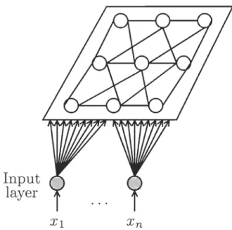
1.4 Thesis Outline. . . . . . . . 2 Artificial Neural Networks (ANNs)

2.1 Introduction . ... 2.2 Learning Paradigms . . . . . . . 2.2.1 Supervised Learning . . 2.2.2 Unsupervised Learning . 2.3 Perceptron... 2.4 Mu1tilayer Perceptron (MLP) . . 2.4.1 Back-propagation .... 2.4.2 Adaptive Learning Rate 2.5 Kohonen Self-Organizing Map 2.6 Hopfield Networks .... . 2.7 Boltzmann Machine .... . 2.8 Radial Basis Function (RBF) 2.9 Conclusion . ... . 3 Fuzzy Logic Systems (FLSs)

3.1 Introduction ... . 3.2 Type-l Fuzzy Logic Systems

ix xiii xiv xix 1 2 3 5 7 9 10 11 11 Il 12 13 13 16 16

20

30

3.2.1 Fuzzification .. ... . 3.2.2 Fuzzy Rule Base ... . 3.2.3 Fuzzy Inference Engine 3.2.4 Defuzzification ... 3.3 Type-2 Fuzzy Logic Systems .. 3.4 Interval Type-2 Fuzzy Logic Systems

3.4.1 Fuzzification.... . . 3.4.2 Fuzzy Rule Base . . . . 3.4.3 Fuzzy Inference Engine 3.4.4 Fuzzy Type Reduction .

3.4.5 Fuzzy Type-Reduced Set Ca1culation 3.4.6 Defuzzification...

3.5 Soft-Computing Based Optimization ... . . 3.5.1 Genetic Algorithms (GA) ... . 3.5.2 Ant Colony Optimization (ACO) Algorithms 3.5.3 Hybrid Systems.

3.6 Conclusion ... ... . 4 Nonlil1ear Control

4.1 Introduction.

4.2 Nonlinear Systems . . . . 4.3 Lyapunov Stability Theory

4.3.1 Autonomous Systems 4.3.2 Non-Autonomous Systems . 4.4 Adaptive Control . . . . . . . . . .

4.4.1 Online Parameter Estimation . 4.4.2 Self-Tuning Regulators . . . . 4.4.3 Gain Scheduling . . . . . . .

4.4.4 Model Reference Adaptive Control (MRAC) 4.5 Sliding-Mode Control.

4.6 Conclusion ... ... .

5 Intelligent Control of Nonlinear Multiple Input Multiple Output Systems 5.1 Introduction ... .

5.2 Neural Learning Algorithm ... . 5.3 Fuzzy Learning Algorithm . . . . . . . . .. . ... . 5.4 A Case of Underactuated Systems: Inverted Pendulums

5.4.1 Modeling . . . . 5.4.2 Friction.. . .. . ... .... 5.4.3 ANN-Based Control of Inverted Pendulums .. 5.4.4 Adaptive Fuzzy Logic Control of Inverted Pendulums 5.5 Hysteresis Compensation for Piezoelectric Actuators ...

x 31 32 32 33 33 35 37 37 37 39 39 41 43 43 44 46 47 49

49

49

67

69

69

76

78

88

5.5.1 Modeling ... . 5.5.2 ANN-Based Control of Piezoelectric Actuators 5.6 Conclusion ... . ... .

94 95 97 6 Control of Robotic Manipulators with Elasticity, Friction, and Disturbance 101

6.1 Introduction... . 101

6.2 Modeling . . . . . . . . . . . 104

6.2.1 Rigid Manipulators . . . . . . 104

6.2.2 Flexible-Joint Manipulators . 106

6.3 Adaptive Control for Rigid Manipulators . . 107

6.3.1 Setup... .110

6.3.2 Results . . . . . . . . . . . . 112 6.4 Adaptive Friction Compensation for Flexible-Joint Manipulators . 112

6.4.1 Setup... . 119

6.4.2 Results . . . . . . . . . . . . . . . . . . . . 121 6.5 Adaptive Disturbance Compensation for Flexible-Joint Manipulators . . ] 26 6.5.1 Results . . . . . . . . . . . . . . . . . 130 6.6 Fuzzy Logic Control of Flexible-Joint Manipulators . . . . . . . . . . . 135

6.6.1 Results... . 139

6.7 Adaptive Type-2 Fuzzy Logic Control for Flexible-Joint Manipulators . 145

6.7.1 Results . 152

6.8 Conclusion . . ... . ... . ... .. ... . 153 7 Lyapunov-Based Control of Permanent Magnet Synchronous Machines 157

7.1 Introduction... . 157

7.2 Modeling . . . . . . . . . . . . . . . . . . ]61

7.3 Observer-based Adaptive Vector Control . . 162

7.3.1 Setup... . 168

7.3.2 Results . . . . . . . . . . . 169

7.4 Observer-based Adaptive Control . . 173

7.4.1 Results . . . . . . . . . . . 180

7.5 Adaptive Control with Uncertain Dynamics 7.5.1 Results . .. ... . 7.6 Sensorless ANN-Based Adaptive Control

7.6.1 Results .. ... . 7.7 Sensorless ANN-Based Vector Control ..

7.7.1 Results ... ... . 7.8 Robust ANN-Based Nonlinear Speed Observer

7.8.1 Results ... . ... . 7.9 Adaptive Fuzzy Logic Control

7.9.1 Results 7.10 Conclusion ... . Xl · 186 .190 · 191 .203 .208 · 216 .223 .225 .228 .234 .241

8 Management and Control of Intelligent Energy Production Systems 8.1 Introduction... .

8.2 Modeling . . . . . . . . . . . . . . . 8.2.1 Bidirectional DC-DC Converters . 8.2.2 Batteries . . .... .. .. .. . 8.3 Adaptive FLC of a DC-DC Boost Convelter

8.3.1 Setup ... . 8.3.2 Results ... . 8.4 Adaptive DC Bus Control. 8.4.1 Setup... 8.4.2 Results . . . . . .

8.5 Observer-based State-of-Charge (SOC) Estimation 8.5.1 Results .... . ... ... .. . . 8.6 Adaptive State-of-Charge (SOC) Estimation 8.6.1 ~etup .. . ... ... 8.6.2 Results . . . . . . . . . . . . . . . 243 .243 .246 .246 .248 .249 .252 .252 .257 .259 .260 .263 .265 .270 .274 .275 8.7 Fuzzy Supervisory Energy Management for Multisource Electric Vehicles . 275

8.7.1 Setup. .279 8.7.2 Results .281 8.8 Conclusion . 282 9 Conclusion Bibliography Publications A Résumé Al Introduction... . . A2 L'identification à base de réseaux de neurones A2.1 Application aux nanosatellites .... A3 Commande adaptative à base d'intelligence artificielle

A3.1 Application à la pendule inversée ... .. .

A3.2 Application aux actionneurs piézoélectriques A4 Commande adaptative des manipulateurs robotiques. AS Les machines synchrones à aimants permanents

A5.1 Commande adaptative .... .. .. . .. . A5.2 Commande intelligente ... .. . .. .. . . A6 Les systèmes intelligents à base d'énergies renouvelables A 7 Conclusion ... . ... ... . xii

285

298

299

Liste des tableaux

2.1 OR gate

. . .

5.1 Inverted PenduIum's parameters 83

5.2 Fuzzy Iogic rules for inverted pendulums . 89

6.1 Manjpulator's physical parameters

(i

= 1,

7.1 PMSM's parameters . .. . .. · 169

7.2 Fuzzy logic rules for PMSMs . .230

8.1 Battery's parameters . . . . .266

8.2 Buck converter's parameters .275

8.3 Fuzzy Logic Rules for n = 2 .279

8.4 Fuzzy Logic Rules for n

=

=

= 3 and SOC

=

=

Table des figures

1.1 Free-flyertestbed atthe CSA ... . 1.2 Compressed air distribution diagram. . . . . . . . . . . . . . . 1.3 Thruster experimental measurements for different air pressures. 1.4 Thrusters diagram of a free-flyer . . . . . . .

1.5 MLP vs. experimental data in training phase 1.6 MLP vs. experimental data for validation 1.7 Thruster model for different air pressures 2.1 Supervised learning

2.2 Unsupervised learning 2.3 Perceptron structure 2.4 Classification example 2.5 Multilayer perceptron

2.6 Single hidden layer multilayer perceptron 2.7 Self-organizing map

2.8 Hopfield network . 2.9 RBF network . . . .

3.1 Block diagram ofa type-l FLS 3.2 Block diagram of a type-2 FLS

3.3 Type-2 Fuzzy Logic Membership Function 3.4 Interval Type-2 Inference Process

4.1 Concepts of Stability . . 4.2 Indirect adaptive control 4.3 Direct adaptive control 4.4 Self-tuning regulator . . 4.5 Gain scheduling ....

4.6 Model-reference adaptive control 5.1 General control structures

5.2 Inverted Pendulum System . 5.3 Stribeck friction model ...

5.4 Lyapunov-based inverted pendulums neural control scheme XIV 4 5 6 6 7 8 8 12 13 14 16 17 17 23 26 28 32 34 35 38 56

60

60

66

66

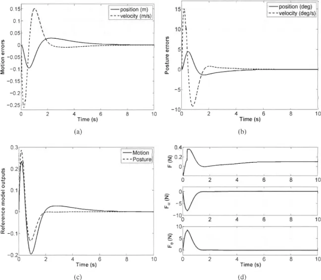
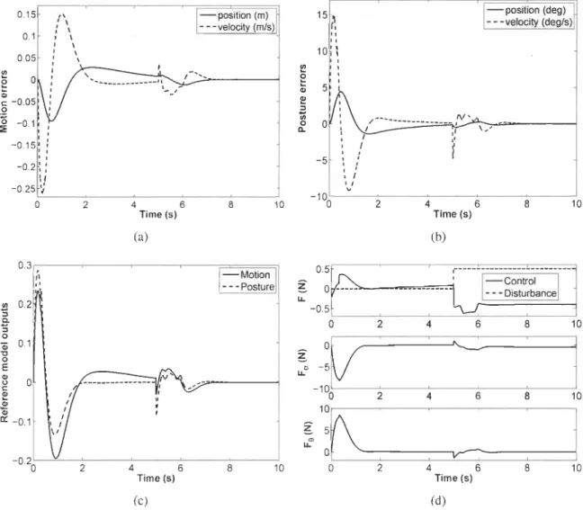
5.5 Motion position and velocity reference signaIs ... 5.6 Inverted pendulum response without ANN controller 5.7 Inverted pendulum response with ANN controller .. 5.8 Inverted pendulum ANN response to disturbance .. 5.9 Lyapunov-based inverted pendulums fuzzy control scheme . 5.10 Motion controller fuzzy membership functions ... . 5.11 Posture controller fuzzy membership functions ... . 5.12 Inverted pendulum FLC response with nominal values 5.13 Inverted pendulum FLC response to disturbance 5.14 Hysteresis characteristic ... . 5.15 Piezoelectric actuator model .. ... .. .... .

5.16 Lyapunov-based piezoelectric actuators neural control scheme 5.17 Position and velocity reference signaIs ... . 5.18 Piezoactuator response without hysteresis compensation. 5.19 Piezoactuator response with hysteresis compensation. 6.1 Flexible-joint model ... .

6.2 Planar robotic manipulator . . . . . . . . . . 6.3 Joints position and velocity reference signaIs 6.4 Manipulator response with nominal values 6.5 Manipulator response with Coulomb friction 6.6 Friction compensation control scheme . . . . 6.7 Friction compensation response with nominal values 6.8 Friction compensation parameters estimate

6.9 Friction estimate with nominal values ... 6.10 Friction estimate with magnified friction .. 6.11 Friction compensation with initial conditions 6.12 Friction compensation with twofold motor inertia . 6.13 Disturbance compensation control scheme .. 6.14 Disturbance compensation with nominal values. 6.15 Disturbance compensation parameters estimate 6.16 Disturbance compensation with higher elasticity 6.17 Disturbance compensation with initial conditions

6.18 Disturbance compensation with higher disturbance magnitude 6.19 Disturbance compensation end-effector trajectory .

6.20 Fuzzy logic control scheme ... . 6.21 Fuzzy membership functions .. . .. . ... . 6.22 Manipulator's FLC position and velocity reference signaIs 6.23 Type-1 and type-2 FLC responses with nominal values 6.24 Type-l and type-2 FLC responses with initial conditions 6.25 Type-l and type-2 FLC responses with twofold inertia .. 6.26 Type-1 and type-2 FLC responses with magnified friction

xv 84 85 86 87 88 89 90 91 92 94 95 96 97 98 99 .106 · 111 · 112 · 113 · 113 · 116 · 122 · 123 · 124 · 125 · 127 · 128 · 129 · 132 · 133 .134 · 136 · 137 · 138 · 139 · 140 · 141 · 142 · 143 · 144 · 146

6.27 6.28 6.29 6.30 6.31 6.32 7.1 7.2 7.3 7.4 7.5 7.6 7.7 7.8 7.9 7.10 7.11 7.12 7.13 7.14 7.15 7.16 7.17 7.18 7.19 7.20 7.21 7.22

Type-l and type-2 FLC responses to load disturbance . Adaptive fuzzy logic control scheme. . . . . . . . . . Adaptive Type-2 fuzzy 10gic control structure ...

Manipulator's adaptive FLC position and velocity reference signaIs

Adaptive type-1 and type-2 FLC responses to varying load's mass and inertia Adaptive type-l and type-2 FLC responses to varying stiffness coefficient Adaptive vector control scheme . . . . . . .

Adaptive control speed reference signal . . . Adaptive vector control with nominal values Adaptive vector control with load variations.

Adaptive vector control with magnified nonlinear friction. Adaptive vector control with parameters variation.

Adaptive control scheme . . . . . . . . . . Adaptive control response with nominal values . . Adaptive control response with load variations . .

Adaptive control response with magnified nonlinear friction Adaptive vector control with parameters variation. . . Disturbance estimation scheme ... . Disturbance estimation response with nominal values. Disturbance estimation response with load variations .

Disturbance estimation response with magnified nonlinear friction Sensorless ANN-based adaptive control scheme ... . ANN-based adaptive control speed reference signal . ... . ANN-based adaptive control response with nominal values ... . ANN-based adaptive control response with load torque disturbance ANN-based adaptive control response in motor and generator mode ANN-based adaptive control response with parameters variation Sensorless ANN-based vector control scheme .

7.23 Sensorless vector control scheme . . ... . .

· 147 · 148 · 148 · 152 · 155 · 156 · 162 · 170 · 171 · 172 · 174 · 175 · 176 · 182 · 183 · 184 · 185 · 186 · 192 · 193 .194 · 195 .204 .205 .206 .207 . 209 .210 · 215 7.24 Non1inear observer speed reference signal . . . . . . . . . 216 7.25 ANN-based vector control response with nominal values . 218 7.26 ANN -based vector control response wi th low inertia J . . 219 7.27 ANN-based vector contTol response with low inductance Ld .220 7.28 ANN-based vector control response with low inductance Lq . 221 7.29 ANN-based vector control response in motor and generator mode . 222 7.30 Robust ANN-based nonlinear speed observer scheme . . . . . . . . 223 7.31 ANN-based nonlinear speed observer response with nominal values. . . 225 7.32 ANN-based nonlinear speed observer response with inductance variations. .226 7.33 ANN-based nonlinear speed observer response with flux variations. . 227

7.34 Adaptive FLC control scheme . . . . 229

7.35 Fuzzy logic membership functions . . . . 230

7.36 Adaptive fuzzy logic control structure . . . . . . . . 231 7.37 Adaptive FLC response with nominal values ... . 235 7.38 Adaptive FLC response with parameters variation. . 237 7.39 Adaptive FLC response with load torque disturbance . 238 7.40 Adaptive FLC response with magnified nonlinear friction . 239

7.41 Adaptive FLC vs. vector control . 240

8.1 Energy production system. . . . . 244

8.2 Electric vehic1e energy system. . 245

8.3 OC-AC power system with a OC-OC bidirectional converter . 246

8.4 OC-OC converter states of operation. . 247

8.5 OC-OC converter . . . . . . . . . . . . . . . . . . . . . . 247 8.6 Equivalent circuit of a battery . . . . . . . . . . . . . . 249 8.7 Adaptive fuzzy control scheme for OC-OC boost converters . 251 8.8 Fuzzy membership functions for a boost converter . . . . . 252 8.9 Adaptive FLC and PI responses with nominal parameters . . 253 8.10 Adaptive FLC and PI responses with a higher load . . . . 254 8.11 Adaptive FLC response with a lower load . . . . . . . . . 255 8.12 Adaptive FLC and PI responses wi th inductor variation . . 256 8.13 Adaptive FLC and PI responses with capacitor variation . 257 8.14 Adaptive OC bus control scheme .. . . .. . . .. . 258 8.15 Classical PI-based cascaded OC bus control scheme .260 8.16 OC bus control under square power demand. . . . 261 8.17 OC bus control under sinusoidal power demand . . . . 262 8.18 Observer-based SOC response with nominal parameters . 267 8.19 Observer-based SOC response with 10 times capacitance . . 268 8.20 Observer-based SOC response with 2 times impedance . 269

8.21 Equivalent circuit of a buck converter . 274

8.22 Converter's control scheme . . . . . . . . . . . . . . 274 8.23 Adaptive SOC response .. .. .. . . . ... . . . 276 8.24 Block diagram of the fuzzy supervisory energy management scheme . . 279 8.25 Input fuzzy membership functions for n = 3 . . . . . . . . . . . . 281 8.26 Fuzzy supervisor response under

±

A.1 Structures de commande générales. . . . . . . . . . . 308 A.2 Structure de commande neuronale pour la pendule inversée . . 309 A.3 Structure de commande floue pour la pendule inversée . . . . 309 A.4 Structure de commande neuronale pour les actionneurs piézoélectriques . 310 A.5 Structure de commande adaptative de compensation de friction . 311 A.6 Structure de commande adaptative neuronale de compensation de perturbation 3] 1 A.7 Structure de commande floue pour les manipulateurs robotiques . . . . . . . 312 A.8 Structure de commande adaptative floue pour les manipulateurs robotiques . . 3] 2

A9 Structure de commande adaptative vectorielle pour les machines synchrones . 313 A.lO Structure de commande adaptative pour les machines synchrones .. ... 314 A.II Structure de commande avec incertitudes pour les machines synchrones . . . . 315 A12 Structure de commande neuronale sans capteur pour les machines synchrones . 315 A13 Structure de commande adaptative neuronale pour les machines synchrones .. 316 A14 Structure de l'observateur neuronale de vitesse pour les machines synchrones . 317 AI5 Structure de commande adaptative floue pour les machines synchrones . 317 A16 Structure de commande flou du convertisseur élévateur . 319 Al7 Structure de commande adaptative du bus CC . . . . . . . . . . . . . . . 319

List of Acronyms

ANN

Artificial neural network Fuzzy logic system Fuzzy logic controller

Microelectromechanical systems MultiLayer perceptron

Radial basis function FootpIint of uncertainty Eevolutionary algorithm Genetic algorithm Ant colony optimization Least squares

Recursive least squares Least mean squares

Model reference adaptive system Model reference adaptive control Canadian space agency

Japanese aerospace exploration agency Single input multiple output

Multiple input multiple output Proportional integral

PD prD FF FBK PMSM EKF DTC MPC PWM SYPWM SOC OCY BMS FNN FNSM Proportional derivative

Proportional integral derivative Feedforward

Feedfback

Permanent magnet synchronous machine Extended Kalman filter

Direct torque control Model predictive control Pulse width modulation

Space vector pulse width modulation State of charge

Open circuit voltage

Battery management system Fuzzy neural network Fuzzy neural sliding mode

Chapitre 1

Introduction

1.1

Motivation

In the literature, control law design approaches for nonlinear systems can be divided into three categories. The first category consists of a nonlinear systems linearization around an operating point of the states [1]. In this case, c1assical linear controllaws are applied for the approximated system. In spite of the control laws simplicity, the control system performance is not guaranteed for the overall system. The second category deals with nonlinear controllers design based on nonlinear systems dynamics. In this category, the characteristics of nonlinear systems are preserved. However, the design approach difficulties arise with the complexity of the nonlinear systems dynamics [2]. Furthermore, these approaches assume a precise mathe-matical system model and tend to work quite well in theory. But, their performance degrades in the presence of varying operating conditions, structured and unstructured dynamical un-certainties, and external disturbances. In real life applications, deriving a precise mathematical model for complex industrial processes might be a difficult task to undertake. In addition, other factors might be unpredictable, such as noise, temperature, and parameters variation. Hence, the system's dynamks cannot be efficiently based on presumably accurate mathematical mod-e1s. The third category implements nonlinear controllers based on computational intelligence too1s, such as artificial neural networks (ANNs) and fuzzy logic systems (FLSs) [3-8]. These

Introduction 2

techniques have been credited in various applications as powerful tools capable of providing robust approximation for mathematically ill-defined systems that may be subjected to struc-tured and unstructured uncertainties [9, 10]. The universal approximation theorem has been the main driving force behind the increasing popularity of such methods as it shows that they are theoretically capable of uniformly approximating any continuous real function to any degree of accuracy. Various artificial neural network and fuzzy logic models have been proposed to solve many complex problems, which have led to a satisfactory performance [11- 14], providing an

alternative to conventional control techniques. To c1early show the power of neural networks, next section presents an application of neural networks in a learning identification strategy for spacecraft formation flying. This technique is used for thrusters' dynamics approximation of a nanosatellite, also called free-flyer. Its effectiveness is investigated using experimental data of a single thruster.

1.2 Spacecraft Formation Flying

Spacecraft formation flying is defined as two or more spaceèrafts flying autonomously in a coordinated fashion and adapting their relative position and orientation to form a forma-tion. It has been identified as an enabling technology with several benefits for space missions and recently became an important field of research in the space industry. Formation flying offers better performance, cost reduction, high failure tolerance, extended mission life, more adaptability to changing mission goals as well as larger spatial coverage. It is expected that

for-mation flying satellites will be more reliable than their single satellite counterparts. Rowever,

this technology faces many challenges in coordination and formation trajectory generation. Environmental disturbances such as gravitational perturbation, atmospheric drag, solar radia-tion pressure and electromagnetic forces make guidance, navigation, and control tasks become more complex for lar'ger formations. Rence, an efficient control algorithm easy to implement on boar'd is required to fulfill the control requirements of a mission.

Introduction

Many researchers investigated propulsion technologies to identify those that maintain high per-formance at sma11 scale. However, independently of the size, thrusters emit caustic propellant exhaust that contaminates neighboring spacecraft. This contamination problem is amplified as the fomlation spacing is reduced. Canadian Space Agency (CSA) initiated, as an international collaboration with the Japanese Aerospace Exploration Agency (JAXA), a feasibility study of JC2Sat-FF nanosatellite mission. It consists of the use of aerodynamic drag to maintain space-craft formation of two nanosatellites. The main advantage is that there is no contamination from propellant exhaust and the missions' lifetime will not be limited by the amount of fuel on board. However, response times to changes in the formation are slow, the relative positions cannot be cont:rolled to a very high accuracy and sorne types of formation are not possible. A theoretical, algorithmic and experimental study of spacecraft formation f1ying is conducted at the CSA, where, a test-bed has been developed to emulate a typical formation f1ying scenario for experimental validation using hardware-in-the-Ioop technology.

Recently, thrusters have received a thorough attention and have been used in many appli-cations such as, high perfomlance surface vessels and underwater robotics appliappli-cations. The nonlinearities within thrusters make the modeling of their dynamics a difficult task to under-take. This has led to the use of a simplified thruster mode1. However, control systems based on this model as well as conventional control techniques often resuIt in poor performance because of the nonlinear and time-varying thruster dynamics. Therefore, an advanced control system with learning capabilities is required to adapt to changes in the thruster dynamics.

1.2.1 Modeling

The free-f1yer of the formation f1ying testbed [15] is shown in Fig 1.1. The testbed is used to emulate a typical formation f1ying scenario with the frictionless nature of space. In space, spacecrafts are free to move in 6 degrees of freedom (3 translations, 3 rotations) and obey the orbital dynamics. However, on the testbed, the free-f1yer can only move in 3 degrees of freedom (2 translations, 1 rotation).

Introduction

FIGURE 1.1 - Free-ftyer testbed at the CSA given by : (the coordinate frames are defined in [15]).

.. FC+F d mixi = . xi xi

.. FC+Fd miYi = yi yi

where,

mi E ]Rn : mass of the {il satellite

li E ]Rn : moment of inertia of the i1h _{satellite about z-axis}

(Xi,Yi) E ]Rn : location of the mass center of the ith satellite in the inertial frame ai E ]Rn : rotation angle of the ith _{satellite about z-axis}

(Fd,

rd)

(F

,

rC)

Assumption 1 We assume a symmetric l1taSS distribution along z-axis.

4

(1.1a) (1.lb) (1.1c)

Introduction

1.2.2 Neural Network Flow Control Valves Identification

This section describes thruster dynamics' learning identification strategy using neural

networks for a free-f1yer. Its effectiveness is investigated using experimental data of a single

thruster. The free-f1yer has eight f10w control valves fed by an air distributor to produce thrust.

Thus, air pressure drops when opening multiple valves at the same time such that only four

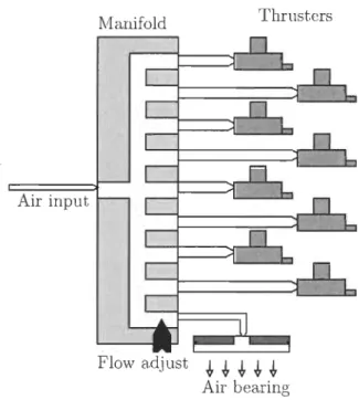
valves are allowed to open simultaneously. Moreover, air distributor also provides air to the

base, to form an air bearing as described in Fig 1.2.

Manifold Thrusters

Air input

* *

* * *

Air bearing

FIGURE 1.2 - Compressed air distribution diagram

The valves are installed on the base of the free-f1yer to provide thrusts to move on

±x

±

y

±

z

pressures (P

=

=

Introduction

different incrementally increasing and decreasing input Nj to capture the hysteresis nature of

the thrusters. It is worth pointing out that step inputs have similar output thrust as the incre-mental inputs. The experiincre-mental measurements are depicted in Fig 1.3 and thrusters diagram in Fig 1.4.

70

60

-

P

80

P

60

₄₀

g8/""

P

40

-

P

20

-

_...

30

20

10

1000

2000

3000

4000

5000

FIGURE 1.3 - Thruster experimental measurements for different air pressures

Thruster

dynamic model

F·

FIGURE 1.4 - Thrusters diagram of a free-flyer Assumption 2 We assume that aIl thrusters are identical.

A feedforward multilayer perceptron (MLP) was used to learn thrusters' dynamics using a variable leaming rate back-propagation algorithm [17]. Experimental data for (P

=

Introduction

left for validation. The feedforward multilayer perceptron has two inputs, two hidden layers

and one output. The first hidden layer has six nodes and the second has eight nodes. The

activation functions used for the hidden and output layers are the sigmoid and linear functions, respectively.

1.2.3 Simulation and Experimental Validation

Fig. ].5 shows the training results, the validation results are depicted in Fig. 1.6, and

Fig 1.7 shows the MLP thrust force for P E [20,80].

70

i:r"

40

-

30

L-t:

20

10

o

1000

2000

3000

4000

FIGURE 1.5 - MLP vs. experimental data in training phase

The following presents an ANN-based modeling strategy for a spacecraft formation flying.

The ANN takes advantage of the merits of the soft-computing technique described in chapter 2

to approximate thrusters' dynarnics using experimental data. The performance of the resultant

strategy shows high approximation accuracy, which confirms the creditentials of such too1s in

providing a robust approximation for mathematically ill-defined systems. They are, therefore,

Introdu

c

tion

20

-

10

.E

-

5

-• -•

o

1000

2000

3000

4000

FIGURE 1.6 - MLP vs. experimental data for validation

70 60 êi50

ir

B

40

.E

30

20

10

.

20<P<80

Or----1000

2000

3000

FIGURE 1.7 - Thruster model (P E [20,80])

4000

Introduction

the design inte11igent adaptive control techniques for complex dynamic systems. Since the stability of neural networks cannot be guaranteed with conventinallearning algorithms such as backpropogation, new Lyapunov-based adaptive learning mechanisms are proposed in this thesis.

1.3 Contributions

Nonlinear dynamic systems are governed by complex dynamics and hence are in-evitably subject to the ubiquitous presence of high, particularly unstructured, modeling nonlin-earities. The presence of such nonlinearities significantly changes the dynamks of nonlinear systems [14]. So, modeling a system's dynamics based on presumably accurate mathematical models cannot be applied efficiently in this case. This raises the urgency to consider alternative approaches for the control of this type of systems to keep up with their increasingly demanding design requirements. The major contributions of this thesis are the design of control structures, adaptation laws and stability proofs for adaptive soft-computing control strategies to achieve :

- Learning and approximation of a priori unknown nonlinear systems.

- Thrusters dynarnics identification for spacecraft formation flying missions. - High uncertainties approximation for inverted pendulums control problem.

- Hysteresis compensation for piezoe1ectric actuators in Microelectromechanical sys-tems (MEMS).

- Stability analysis for soft-computing techniques.

- Lyapunov-based adaptive learning mechanism for neural networks. - Stable adaptation technique for fuzzy systems in the sense of Lyapunov.

- Lyapunov stable adaptive control strategies for electromechanical systems such as robotic manipulators.

- Adaptive friction compensation to cope with its nonlinearities.

- Disturbance attenuation to achieve robustness to unstructured uncertainties.

manipula-Introduction

tors.

- Parameters adaptation to obtain robustness to parametric uncertainties.

- High performance and robustness in PMSM drives.

- Friction and load torque estimation for high tracking accuracy.

- Adaptive control techniques for robustness to parametric uncertainties.

- Soft-computing based approaches for high tolerance to unstructured uncertainties.

- Speed estimation strategies.

- High efficiency for energy production systems.

- Accurate state of charge estimation for battery management systems.

- Soft-computing based adaptive control for power converters.

- Adaptive DC bus voltage control to improve energy transfer efficiency.

1

.

4 Thesis Outline

The thesis is organized as foIlows. Chapters 2 to 4 present the background of artifi-cial neural networks theory, fuzzy logic systems, neuro-fuzzy systems along with genetic and ant colony algorithms as soft-computing techniques, and nonlinear control systems. Chapter 5 presents Lyapunov-based adaptation strategies for neural networks and fuzzy systems. These

techniques are applied to the well-known inverted pendulum problem. The ANN

Lyapunov-based adaptation technique is also applied to piezoelectric actuators. In chapter 6, modeling of

robotic manipulators with friction and joint el asti city is presented as weIl as many advanced control strategies with their results. In chapter 7, we present several speed control and

estima-tion strategies for permanent magnet synchronous machines along with their stability proofs

and results. Advanced adaptive techniques are presented in chapter 8 for energy production

Chapitre 2

Artificial Neural Networks (ANNs)

2.1 Introduction

An artificial neural network (ANN) is a computational model that processes informa-tion using interconnected artificial neurons. As such, it mimics the structure and functional characteristics of biological neural networks of a brain in the way information is interpreted, the ability to learn, generalize and adapt to new situations. The ANN's inherent parallel nature increases infonnation processing speed by distributing the calculations among many neurons. This chapter focuses on popular ANN models.

2.2 Learning Paradigms

An ANN, in its simplest form, has a set of inputs, connection weights, and outputs. The inputs are multiplied by the weight and are then summed before applying an activation function to the summed value. This activation level becomes the neuron 's output and can be either an input for other neurons, or an output for the network. The learning is achieved by adjusting the weights to minimize the difference between the ANN and desired (training data) outputs. ANN can also be viewed as an adaptive system that changes its structure during the learning phase based on a set of training data. It can be used to model complex relationships

Artificial Neural Networks (ANNs) 12

between inputs and outputs or to find patterns in data.

There are two approaches to train a neural network, supervised and unsupervised learning. Supervised learning involves a mechanism, also called teacher, to provide the network with the desired output or the network's performance, such as a co st function. On the other hand, unsu-pervised learning does not have a function to be learned by the network but rather a continuous interaction with the environment.

2

.

2

.

1 Superv

i

sed Learn

i

ng

In supervised learning, input-output training sets are provided to the network, which

processes the information and computes the errors based on ilS resulting outputs. These errors are then propagated back through the network to adjust its weights. This process continues as

the connection weights are ever refined until convergence. It is noteworthy that training sets

with not enough infoTI11ation may not lead to convergence and too many layers and nodes make the network memorize the data instead of learning from it. The supervised learning scheme is depicted in figure. 2.1.

En

v

ir

o

nm

e

n

t

"---r-~

T

eac

h

e

r

Artificial Neural Networks (ANNs) 13

2.2.2 Unsupervised Learning

In unsupervised leaming, the network is provided with only input training sets. In real life, exact training sets do not exist for aIl situations. Hence, this type of leaming aims to provide the network with the ability to adapt to the environment and learn from it, such as self-organizing map and reinforcement learning. The supervised leaming scheme is depicted in figure. 2.2. As training data is not available, the network leams through a minimization of a co st function also called "critic".

Input

En

v

ir

a

nm

e

n

t

Cri

t

i

c

Actual output

FIGURE 2.2 - Unsupervised leaming scheme

2.3 Perceptron

The perceptron was first introduced by Rosenblatt in 1958 along with the mechanism to adjust its weights [18]. It is a very simple binary neural network with a single neuron. The perceptron uses supervised learning process to solve basic logical operations like AND or OR. However, it cannot solve more complicated logical operations, like the XOR problem. It is often used for pattern classification purposes. Figure. 2.3 shows a typical perceptron structure and its supervised training algorithm is described in algorithm 1.

Artificial Neural Networks (ANNs)

FIGURE 2.3 - Perceptron structure

Aigorithm 1: Perceptron (Delta mie)

begin

- Initialize the weight vector Wi and the threshold

e

repeat repeat

14

- Present an input vector

x(k)

,

xnl

d(k)

k.

- Compute the perceptron output

y(k)

(Xi Wi) -

e)

.

0>

e

f(

- Adapt the weight vector by the following :

e(k)

d(k)

- y(k)

,

T/

<

wi(k+

1)

wi(k)

+

T/e(k)xi(k)

until aIl training instances are finished.

until convergence or satisfactory peiformance is reached.

end TABLE 2.1 - OR problem XI 1 X2 Il y 0 0 0 0 1 1 1 0 1 1 1 1

Artificial Neural Networks (ANNs)

Consider a two-input perceptron to solve the OR problem in table 2.1.

InÏtialize the weights and the threshold to small random values:

WJ

=

=

e

=

Set the learning rate to : 17 = 0.15.

Present the network with random patterns:

- First pattern: (pattern 3

=

Compute the output

y(k)

=

e)

=

=

=

Compute the error

e(k)

=

d(k) -

y(k)

=

=

Since

e(k)

=J.

Wl

(k+

=

(k)

17e(k)x\

(k)

=

=

w2(k+

=

w2(k)

17e(k)X2(k)

=

=

- Second pattern : (pattern 2

=

y(k)

=

=

=

e(k)

W\

(k

=

=

w2(k+

=

=

- Third pattern : (pattern 4

=

y(k)

=

=

=

e(k)

- Fourth pattern: (pattern 1

=

y(k)

=

f(

=

f(

=

e(k)

15

Recall,

y(k)

e)

e).

Artificial Neural Networks (ANNs) 16

Therefore,

w)

e

X 2 = X ) +

-W2 W2

It is noteworthy that the slope of the line is determined by the weights and the threshold determines the offset. Thus, the perceptron represents a linear discriminant function. A geo-metrical representation before and after training is given in Fig. 2.4.

X2 _\ X2

1

X

,

\1

_X

\~\

1

\

1

FIGURE 2.4 - Classification exarnple : (a) before training; and (b) after training.

2

.

4 Multilayer Perceptron (MLP)

The multi-Iayer-perceptron (MLP) was first introduced by Minsky and Papert in 1969 [18J. It is an extended version of the single layer perceptron as it may have one or more hidden lay-ers. Whilst a perceptron forms a half-plane decision region, a MLP forms arbitrarily complex decision regions to separate various input patterns. Due to its extended structure, a MLP is able to solve every logical operation, including the XOR problem. Figure. 2.5 shows a typical MLP structure.

2.4.1 Back-propagation

Consider a single hidden layer neural network with n inputs, p hidden nodes, and m

Artificial Neural Networks (ANNs)

Input

layer Hidden layerl Hidden layer2 Output layer FlOURE 2.5 - Multilayer perceptron structure

Input

layer Hidden layer Output layer

FlOURE 2.6 - Single hidden layer multilayer perceptron

Artificial Neural Networks (ANNs)

We can describe the input-output relationship by

with,

p

Vk(t)

E

Wkj(t) Oj(t)

j=l

n

Uj(t)

E

wji(t) Xi(t)

xJt)

Yk(t)

The back-propagation is a supervised learning algorithm mainly used by MLPs to minimize a co st function that can be described as

(2.5) with,

(2.6)

where,

ek(t)

dk(t)

The back-propagation algorithm adapts the weights using a gradient descent technique, where the gradient is computed by

aÇ

(t)

aWkj(t)

aÇ

(t)

aWji(t)

aÇ

(t)

aek(t) aYk(t) aVk(t)

-aek(t) aYk(t) aVk(t) aWkj(t)

aç(t) aoj(t) aUj(t)

-aoj(t) au

j(t)

aWji(t)

(2.7) (2.8)

Artificial Neural Netwarks (ANNs) 19

Differentiating (2.5) with respect ta

ek(t)

(2.9) Differentiating (2.6) with respect ta

Yk(t)

(2.10) Differentiating (2.1) with respect ta

Vk(t)

(2. II ) Differentiating (2.2) with respect to Wkj(t) yields,

(2.12) Differentiating (2.5) with respect to

0 j(t)

(2.13) Substitute (2.1) in (2.6) yields,

Therefore,

(2.14) Differentiating (2.2) with respect to

0 j(t)

Artificial Neural Networks (ANNs) 20

Differentiating (2.3) with respect to Uj(t) yields,

(2.16)

Differentiating (2.4) with respect to

Wji(t)

(2.17) Substitute (2.9), (2.10), (2.11), and (2.12) in (2.7) and (2.13), (2.16), and (2.17) in (2.8) yields,

where, Oj(t) and ok

(t)

The weights correction are defined by the delta rule

where, Tl is the learning rate. Therefore, the neural network weights are computed as follows,

Wkj(t

+

1)

Wkj(t)

+

wji(t

+

1)

wji(t)

+

2

.

4

.

2 A

da

ptive Learning Rate

The standard backpropagation algorithm using a constant 1earning rate cannot handle

aIl the error surfaces. In other words, an optimallearning rate for a given synaptic weight is not necessarily optimal for the rest of the network's synaptic weights. Henceforth, every adjustable

Artificial Neural Networks (ANNs) 21

network parameter of the cost function should have its own individuallearning rate parameter. Moreover every learning rate parameter should be allowed to vary at each iteration because the error surface typically behaves differently along different regions of a single-weight

dimen-sion [18]. The current operating point in the weight space may lie on a relatively flat portion of the error surface along a particular weight dimension. In such a situation where the derivative of the co st function with respect to that weight maintains the same algebraic sign, which means pointing in the same direction, for several consecutive iterations of the algorithm, the learning rate parameter for that particular weight should be increased. When the current operating point in the weight space lies on a portion of the error surface along a weight dimension of interest that exhibits peaks and valleys (i.e., the surface is highly irregular), then it is possible for the derivative of the cost function with respect to that weight to change its algebraic sign from one iteration to the next. To prevent the weight adjustment from oscillating, the learning rate parameter for that particular weight should be decreased appropriately when the algebraic sign

of the derivative of the cost function with respect to a particular synaptic weight alternates for several consecutive iterations of the algorithm [18]. It is noteworthy that the use of a different time-varying learning rate parameter for each synaptic weight in accordance to this approach modifies the standard backpropagation algorithm in a fundamental way.

2.5 Kohonen Self-Organizing Map

The Kohonen self-organizing map, also called the Kohonen feature map, was tirst in-troduced by Teuvo Kohonen in 1982 [18]. It is one of the most used neural network models

for data analysis. It can also be applied to other tasks where neural networks have been tried

successfully. A self-organizing map (Fig. 2.7) consists of two layers, an input layer and an

output layer, called a feature map, which represent the output vectors of the output space. The

weights of the connections of an output neuron j to aIl the n input neurons, form a vector W j in

an n-dimensional space. The input values may be continuous or discrete, but the output values are binary only.

Artificial Neural Networks (ANNs) 22

The output neurons learn during the training phase to react to inputs that belong to sorne

clusters to represent typical features. This characteristic is inspired from the fact that the

brain is organized into regions that correspond to different sensory stimuli. Therefore, a

self-organizing map is able to extract abstract infol111ation from multidimensional array and

repre-sent it as a location, in one, or more dimensional space.

ln the training phase, the output layer neurons are competitive. A neuron has a strong

exci-tatory connection to itself and the excitatory level decreases within a certain radius when

mov-ing away to its neighbormov-ing neurons. Beyond this radius, a neuron either inhibits the activation

of the other neurons or does not influence them. This scheme is called the "winner-takes-all",

where a competition between neurons yields only one winner neuron that represents the class

or the feature to which the input vector belongs. The self-organizing map structure is depicted

in Fig. 2.7.

The unsupervised training algorithm for self-organizing map is described in algorithm 2 :

Algorithm 2: Self-organizing map unsupervised training begin

- Initialize the weight vector W j to small random values.

repeat repeat

- Present an input vector x at time t.

- Compute the distance dj(t) = E(x(t) - Wj(t))2.

- Declare the neuron with the smallest distance as a winner.

- Change the weight vector within the neighbourhood area R :

.

(

l)-{

wJ _t

+

-

7J is the learning rate.

- Decrease 7J and R in time.

until al! training instances are finished.

until convergence or satisfactOlY performance is reached.

end

Example: (classification problem)

Artificial Neural Networks (ANNs)

Input

layer

FIGURE 2.7 - Self-organizing map structure

Initialize the weights to small random values: 0.2 0.1

w = 0.1 0.3

0.4 0.2 Set the radius as : R = O.

Set the 1earning rate as : 17 (0)

=

(t

+

=

(t)

Present the network with input vectors :

- First pattern: (0,1,0)

Compute the distance :

dJ

=

+

=

d2

=

=

w2(k+

w2(k)

+

(Xi

-

wi2(k))

- Second pattern: (0,0,1)

Compute the distance :

Artjficial Neural Networks (ANNs)

d]

=

+

+

=

d2

=

+

+

=

Adapt the weights of the winner node (1) :

w]

(k

+

(k)

+

(k))

- Third pattern: (1,0,0)

Compute the distance :

d]

=

+

+

=

d2

=

+

+

=

Adapt the weights of the winner node (1) :

wl(k+

=

w] (k)

+

(k))

=

- Reduce the learning rate: 1](t

+

- The new weight matrix :

0.47 0.06

W = 0.03 0.58

0.38 0.12

- Go for another iteration.

After many iterations, the weight matrix converges to the following :

0.5 0

w=

0.5 0

24

The first c1uster converges to the average of the two input vectors (0,0,1) (1,0,0), while third

Artificial Neural Networks (ANNs) 25

2.6 Hopfield Networks

Hopfie1d network was first introduced by John Hopfield in 1982 [18]. It is a fully con-nected feedback network, where each neuron is concon-nected to aIl other neurons and there is no differentiation between input and output neurons. The Hopfie1d network structure is depicted in Fig. 2.8. There are variants of realizations of a Hopfield network. Every neuron j, j = 1,2, ... ,n

in the network is connected back to every other one, except itself. Input patterns Xj are supplied

to the external inputs Ij and cause activation of the external outputs. The response of such a

network, when an input vector is supplied during the recall procedure, is dynamic, that is, after

supplying the new input pattern, the network ca1culates the outputs and th en feeds them back

to the neurons ; new output values are then ca1culated, and so on, unti1 equilibrium is reached. Equilibrium is considered to be the state of the system when the output signaIs do not change for two consecutive cycles, or change within a small constant. The weights in a Hopfield net-work are symmetrical for reasons of stabi1ity in reaching equilibrium, that is, Wij = Wji. The

network is of an additive type, that is,

{ l,

0 '

-1 - 0 or-l,

where, Bj is a threshold for the

fh

ifUj > Bj

otherwise

A dynamica1 energy function E of a Hopfield network is defined at a moment t as

1 n n

E(t)

-2

L L

(wij(t) Oi(t) Oj(t)),

i=l j=l

Artificial Neural Networks (ANNs)

26

network to local minima states when the weights of a Hopfield network are computed by

111

wij =

E

p=1

where,

xi

function is a stable state for the network.

The weights update might be done according to the following modes:

- Asynchronous updating : Each neuron changes its state at a random moment with respect to other neurons.

- Synchronous updating : AlI neurons change their state simultaneously at a given time. - Sequential updating : AlI neurons change their state sequential1y, i.e., only one neuron

changes its state at a given time.

FIGURE 2.8 - Hopfield network structure

2.7

Boltzmann Machine

The Boltzmann machine was developed by Hinton and Sejnowski in 1983 to overcome the local minima prob1em [18]. It uses a variable called temperature to calculate the activation

Artificial Neural Networks (ANNs)

value of a neuron as a statistical probability

Oi

=

=

Oi = 0, with a probability (1-Pi)

27

where Ui is the network's input to the eh neuron, calculated as in the Hopfield network. This model is called a Boltzmann machine because of its similarity with the process of

anneal-ing in metallurgy, where temperature T decreases during the recall process. By changing the temperature, we shake the neural network to enable a jump from a local minima and a move towards a global minimum attractor.

2.8 Radial Basis Function (RBF)

Radial basis functions were first introduced by Powell in 1989 [18]. RBF network is

an excellent approximator used for curve fitting problems and its learning is equivalent to finding a multidimensional function that provides a best fit to the training data. Moreover, it can be trained easily and quickly. The main advantage of RBF network is that the output

layer weights are adjusted through linear optimization, whereas the hidden layer weights are adjusted through a nonlinear optimization. As depicted in Fig. 2.9, the RBF network output can be expressed using the Gaussian function and the weighted sum method,

1 Yk=LWk)</», k=I,2, ... ,m )=1

(

IIXi-C)112)

.

where n, i, and m are the number of input, hidden, and output nodes', respectively, Xi is the

ith input vector of the training set and wk) is the weight connecting the j'h hidden node to the

k.th output node, </», ci, and (J) are the /11 Gaussian function, center, and standard deviation,

neu-Artificial Neural Networks (ANNs)

28

rons needed in the second layer. Rowever, appropriate RBF eenters and widths selection can improve the accuracy and speed of the network. Renee more efficient RBF networks are built by the redistribution of centers to locations where input training data are meaningful.

Input

layer Hidden layer Output layer

FIGURE 2.9 - RBF network structure

There are three major approaches to detennine the eenters. In the tirst approach, the loca-tions of the centers are tixed and chosen randomly from the training data. This method can be useful if the training data are distributed in a representative manner for the specitied problem. In the second approach, the radial basis functions can move the locations of their centers in a

self-organized fashion. Renee, the eenters of radial basis functions are plaeed in the regions

of the input spaee where important data exist. In the third approach, the eenters of the radial basis functions are obtained by a supervised leaming proeess. It defines a co st function to be rninimized using an elTor-COlTection leaming scheme such as a gradient-descent procedure.

Artificial Neural Networks (ANNs) 29

2.9 Conclusion

ANNs have received a thorough interest from man y researchers as they are able to learn

a system's behavior from its input-output data. These learning and generalization capabilities

enable ANNs to more effectively address nonlinear time-varying complex problems. Thus far, MLP remains one the most popular ANNs used in control applications with backpropagation

aIgorithm for weights adaptation. However, this aIgorithm is based on gradient or steepest

de-scent methods. These methods have a serious drawback as they are not suitable for aIl types of

swfaces. Therefore, the convergence and stability of such approaches cannot be guaranteed. In

this thesis, the MLP is used for its simplicity and its stability issues are addressed by proposing

new Lyapunov-based adaptation techniques as an alternative to c1assic gradient-based

meth-ods. On the other hand, fuzzy logic systems are also good candidates for nonlinear dynamic

systems. They have been successfully used in many real-world applications. Therefore, the