HAL Id: tel-00835500
https://tel.archives-ouvertes.fr/tel-00835500v3
Submitted on 5 Jan 2017
HAL is a multi-disciplinary open access
archive for the deposit and dissemination of sci-entific research documents, whether they are pub-lished or not. The documents may come from teaching and research institutions in France or abroad, or from public or private research centers.
L’archive ouverte pluridisciplinaire HAL, est destinée au dépôt et à la diffusion de documents scientifiques de niveau recherche, publiés ou non, émanant des établissements d’enseignement et de recherche français ou étrangers, des laboratoires publics ou privés.
Shear coordinates on the super Teichmüller space
Fabien Bouschbacher
To cite this version:
Fabien Bouschbacher. Shear coordinates on the super Teichmüller space. Differential Geometry [math.DG]. Université de Strasbourg, 2013. English. �NNT : 2013STRAD010�. �tel-00835500v3�
UNIVERSITÉ DE STRASBOURG
ÉCOLE DOCTORALE MSII (ED n°269)
IRMA, UMR 7501
THÈSE
présentée par :Fabien BOUSCHBACHER
soutenue le : 25 juin 2013
pour obtenir le grade de :
Docteur de l’université de Strasbourg
Discipline/ Spécialité
: Mathématiques
Des coordonnées de décalage sur le
super espace de Teichmüller
THÈSE dirigée par :
M. FOCK Vladimir Professeur, Université de Strasbourg
RAPPORTEURS :
M. RESHETIKHIN Nicolai Professeur, U.C. Berkeley
Mme SERGANOVA Vera Professeur, U.C. Berkeley
AUTRES MEMBRES DU JURY :
M. COSTANTINO Francesco Maître de Conférences, Université de Strasbourg
M. GUICHARD Olivier Professeur, Université de Strasbourg
Shear coordinates on the super-Teichm¨uller space
Fabien BOUSCHBACHER
Institut de Recherche Math´ematique Avanc´ee
Universit´e de Strasbourg et C.N.R.S (UMR 7501)
7, rue Ren´e Descartes
67084 STRASBOURG Cedex
`
On ne peut jamais tourner une page de sa vie sans que s’y accroche une certaine nostalgie.
`
Remerciements
Selon Pierre Dac,
Il faut une infinie patience pour attendre toujours ce qui n’arrive jamais.
De mon cˆot´e, j’ai bien cru que ce jour n’arriverait jamais... Je tiens `a exprimer toute ma gratitude `a mon directeur de th`ese, Vladimir Fock. Durant ces quatre ann´ees, avec beaucoup de gentillesse, il a su se rendre disponible et encadrer ce travail avec une grande patience. Je tiens aussi `a le remercier pour m’avoir laiss´e choisir cette route vers ce sujet, `a la fin d’une premi`ere ann´ee difficile.
Pendant ces ann´ees, j’ai aussi eu la chance de travailler aux cˆot´es de Fran¸cois Costantino, co-encadrant de cette th`ese. Je tiens `a le remercier chaleureusement pour son soutien ind´efectible. Ce travail doit beaucoup `a son investissement, ses nombreuses relectures et sa rigueur. Sans lui, ce manuscrit n’aurait jamais vu le jour.
J’aimerais ensuite remercier les rapporteurs qui ont accept´e de consacrer leur temps `a la lecture de cette th`ese : merci `a Vera Serganova et Nicolai Reshetikhin pour l’int´erˆet qu’ils portent `a ce travail. Merci `a Olivier Guichard et Anton Zorich qui me font l’honneur de si´eger dans mon jury. La constitution de ce jury n’a pas ´et´e des plus simples: merci au projet ANR ETTT qui a permis de r´eunir tout le monde ici aujourd’hui. Un grand merci `a Hubert Rubenthaler et `a l’´ecole doctorale MSII pour leur contribution dans l’organisation de cette soutenance.
Je profite aussi de ce moment pour remercier toute la famille quantique. Merci `a Christian Kassel, Benjamin Enriquez, Gw´ena¨el Massuyeau et Pierre Baumann qui ont su m’´ecouter avec attention lorsque j’en ai eu besoin.
Durant ces quatre ann´ees, j’ai eu la chance de m’int´egrer dans des ´equipes p´edagogiques o`u r´egnaient la bonne humeur. Merci `a tous ceux avec qui j’ai pu travailler chaque ann´ee. Je souhaite aussi remercier tous le personnel administratif de l’IRMA et UFR de Math´ematique et d’Informatique qui a rendu tant de choses plus l´eg`eres.
C’est avec un peu de nostalgie que je remercie ceux qui, il y a quatre ans, m’ont ac-cueilli `a bras ouverts dans cette joyeuse bande de doctorants et assimil´es : Anne-Laure, Audrey, Aurore, ´Elodie, H´el`ene, Adrien, Aur´elien, Florian, Ghislain, Kees, R´emi, Scoum, Thomas et Vince (j’en oublie sˆurement : pardon !) et merci `a tous les autres qui m’ont
vi
support´e jusqu’`a ce jour, Charlotte, J´erˆome, Valentina, Ambroise, Alexandre, Auguste Olivier, Enrica, Romain, Alain, Nicolas,... Pendant trois ans j’ai eu la “lourde” tˆache de m’occuper du s´eminaire doctorant, merci `a tous pour votre pr´esence et votre investisse-ment. Si vous lisez ces quelques lignes, commencez `a penser `a un successeur...
Et puis, que serais-je sans l’amour incommensurable et le soutien sans faille de mes proches ? Merci Maman, merci Papa, je ne sais comment vous remercier pour tout ce que vous avez fait pour moi. Merci `a mes sœurs Laurence et ´Emilie qui ont su (et sauront) me soutenir en toute situation. Merci aussi `a Tophe et Manu pour ces nombreuses discussions, parfois un peu surr´ealistes, le dimanche midi. J’ai aussi une pens´ee ´emue pour mes grands-parents qui m’ont accompagn´e tout au long de mon parcours.
Le d´ebut de cette th`ese co¨ıncide avec le d´ebut d’une autre histoire. Il y a presque quatre ans maintenant que Fr´ed´erique et Marc, mes beaux-parents, m’ont accueilli comme un fils. Je ne pourrai jamais assez les remercier pour cela. Un grand merci `a ma belle-famille pour leurs encouragements.
Enfin, je n’aurai pas assez de place ici pour lui exprimer ma gratitude ; pas assez de mots pour expliquer ce que je lui dois. Alors je vais rester sobre et aller au plus simple :
Contents
Remerciements v
Introduction ix
English introduction xv
1 Teichm¨uller spaces 1
1.1 The Teichm¨uller space of Riemann surfaces of type (g, k, m) . . . 1
1.2 Two extensions to open ciliated surfaces . . . 3
1.2.1 Ciliated surfaces . . . 3
1.2.2 Teichm¨uller spaces of surfaces with holes. . . 5
2 Supermanifolds 9 2.1 Super algebras . . . 9
2.1.1 Super vector spaces and super commutative algebras . . . 9
2.1.2 Modules of super algebras and superspaces . . . 10
2.2 Supersmooth functions on Rn|m . . . 12
2.2.1 The DeWitt topology . . . 12
2.2.2 Supersmooth functions on Rn|m . . . 12
2.3 The definition of DeWitt supermanifolds . . . 13
2.3.1 The topology of a DeWitt super-premanifold . . . 14
2.3.2 The body of a DeWitt super-premanifold . . . 14
2.3.3 The algebro-geometric approach to supermanifolds . . . 14
2.4 Further examples . . . 15
2.4.1 Real super projective spaces . . . 15
2.4.2 The super upper half-plane . . . 16
2.4.3 The group SpO(2|1)(R) . . . 16
2.5 The super-Teichm¨uller space . . . 19
2.5.1 Canonical system of generators of ⇡1(S) and super-Fuchsian models 19 2.5.2 Definition of the super-Teichm¨uller space . . . 20
viii Contents 3 Spin structures, quadratic forms and Kasteleyn orientations 21
3.1 Spin structures and quadratic forms . . . 21
3.2 Kasteleyn orientations, dimer configurations and spin structures . . . 22
4 Construction of coordinates on the super-Teichm¨uller X space 27 4.1 Invariant and pseudo-invariant . . . 27
4.1.1 The super cross-ratio, the even invariant . . . 28
4.1.2 The odd pseudo-invariant . . . 28
4.2 Refinement of the odd invariant . . . 28
4.3 The super-Teichm¨uller X-space of a surface . . . 31
4.3.1 Definition . . . 31
4.3.2 Lifting ideal triangulations . . . 31
4.3.3 Coordinates on the super-Teichm¨uller X-space . . . 33
4.4 Reconstruction of the morphism . . . 35
5 Superflips and superpentagons 43 6 Poisson structures 53 6.1 Poisson manifolds and Poisson supermanifolds . . . 53
6.1.1 Poisson manifolds . . . 53
6.1.2 Poisson supermanifolds . . . 53
Introduction
Contexte
Le probl`eme de la param´etrisation des structures complexes sur une surface donn´ee re-monte `a l’´epoque de Riemann. Ce dernier d´etermina de mani`ere informelle le nombre de param`etres n´ecessaire `a la description des classes de surfaces de Riemann `a biholo-morphismes pr`es. Teichm¨uller d´emontra, quatre-vingts ans plus tard, que ces param`etres pouvaient ˆetre utilis´es en tant que coordonn´ees sur une cellule, appel´ee espace de Teich-m¨uller, dont le quotient par une action naturelle du groupe d’hom´eotopie est l’espace des modules de Riemann.
L’espace de Teichm¨uller, d´efini `a partir des surfaces marqu´ees, apparaˆıt implicite-ment dans les travaux de Klein et Poincar´e sur les groupes fuchsiens. Le th´eor`eme d’uniformisation de Klein, Poincar´e et Koebe fournit une bijection entre les classes d’iso-morphisme de surfaces de Riemann hom´eomorphes `a Sg et les classes d’isom´etrie de
sur-faces hyperboliques hom´eomorphes `a Sg, o`u Sg est une surface compacte de genre g 2.
`
A l’aide de m´ethodes bas´ees sur ce th´eor`eme, Fricke construit un syst`eme de coordonn´ees sur l’espace de Teichm¨uller Tg de Sg et montre qu’il s’agit d’une cellule de dimension r´eelle
6g 6.
Il existe d’autres param´etrisations de l’espace de Teichm¨uller et Thurston [32] d´e-montre, au milieu des ann´ees 80, que toute structure hyperbolique sur une surface point´ee peut ˆetre d´ecrite par l’a↵ectation d’un nombre r´eel strictement positif `a chaque arˆete d’une triangulation id´eale de la surface (c’est-`a-dire une d´ecomposition de la surface en triangles de sorte que les sommets de la triangulation sont exactement les pointes ; un exemple est donn´e Chapitre 1, Figure 1.1). Ces param`etres de d´ecalage encodent la fa¸con de recoller deux triangles id´eaux de la triangulation. Les coordonn´ees de d´ecalage ont ´et´e d´evelopp´ees par Bonahon [4] et Fock [13] qui montrent notamment comment exprimer di↵´erentes structures sur l’espace de Teichm¨uller `a l’aide de ces derni`eres. Les coordonn´ees d´ependent de la triangulation id´eale, mais lorsqu’on change de triangulation par un mouvement ´el´ementaire, appel´e flip, les coordonn´ees changent de fa¸con bien contrˆol´ee. Un th´eor`eme dˆu ind´ependamment `a Harer [17], Strebel et Penner [28] assure que toute triangulation id´eale peut ˆetre obtenue `a partir d’une autre en appliquant une s´equence de ces mouvements qui satisfont trois types de relation (involution, commutation lointaine et l’importante
x Introduction relation du pentagone). En particulier les coordonn´ees de Thurston-Bonahon-Fock-Penner permettent d’encoder la structure de Poisson sur l’espace de Teichm¨uller de fa¸con agr´eable et les changements de coordonn´ees pr´eservent cette structure.
Ces coordonn´ees se r´ev`elent ˆetre particuli`erement utiles au d´eveloppement de la re-cherche sur les espaces de Teichm¨uller et leurs analogues en rang sup´erieur :
1. La quantification des espaces de Teichm¨uller a ´et´e construite en d´eformant l’alg`ebre engendr´ee par les coordoonn´ees de d´ecalage dans la direction de la structure de Poisson [6].
2. L’´etude des espaces des modules des repr´esentations du groupe fondamental d’une surface dans d’autres groupes classiques comme SLn(R) a ´et´e d´evelopp´ee par Fock
et Goncharov [12] qui ont d´efini des coordonn´ees sur ces espaces (judicieusement d´ecor´es) et ´etabli quelles ´etaient leurs transformations lorsqu’un flip ´etait appliqu´e. Cela leur a permis d’identifier combinatoirement une composante “positive” corres-pondant `a celle de Hitchin.
Le concept de supervari´et´e, g´en´eralisant celui de vari´et´e classique en ajoutant des co-ordonn´ees anticommutatives aux cartes locales, a ´et´e introduit par les physiciens ´etudiant la supersym´etrie. Il existe di↵´erentes fa¸cons de d´efinir les supervari´et´es. Nous nous int´eressons dans notre ´etude `a l’approche de DeWitt [10], app´el´ee approche concr`ete par Rogers [30, 31]. Grosso modo, dans l’approche de DeWitt, une supervari´et´e est une vari´et´e qui est localement isomorphe `a un superespace not´e Rn|m, dont les coordonn´ees sont `a valeurs dans une alg`ebre supercommutative, alg`ebre grassmannienne (cf. Defini-tion 2.1.2). En particulier, cela conduit `a la d´efiniDefini-tion des super surfaces de Riemann, qui sont fondamentales en th´eorie des cordes supersym´etriques : elles sont les surfaces d’univers de la th´eorie. Dans le formalisme de Poliakov de la th´eorie de cordes bosoniques (cf. [29, 9]), le calcul de la fonction de partition d’une corde peut ˆetre e↵ectu´e en int´egrant sur l’espace des modules de surfaces de Riemann. Dans le cas supersym´etrique, cet espace des modules devrait ˆetre remplac´e par son superanalogue.
Une super surface de Riemann peut ˆetre vue comme une classe de conjugaison de mor-phismes de son groupe fondamental dans un groupe de matrices, not´e SpO(2|1), dont les coefficients appartiennent `a l’alg`ebre grassmannienne. Ce groupe se projette sur SL(2,R), on peut par cons´equent lui associer sa r´eduction repr´esent´ee par une surface de Riemann classique avec un relev´e de l’holonomie de PSL(2,R) `a SL(2, R) : une structure spin. Le super espace de Teichm¨uller est une supervari´et´e param´etrant les super surfaces de Riemann ayant la mˆeme topologie. Cette th´eorie des super espaces de Teichm¨uller a ´et´e d´evelopp´ee dans le cas des surfaces ferm´ees de genre g [9, 18]. Le besoin d’une structure spin fait que le super espace de Teichm¨uller admette plusieurs composantes connexes. Crane et Rabin [9] and Hodgkin [18] ont d´emontr´e que chaque composante ´etait une “super boule” de dimension (6g 6|4g 4).
Dans cette th`ese, nous avons pour but de construire des coordonn´ees de d´ecalage pour les super surfaces de Riemann point´ees munies d’une triangulation id´eale ainsi que de d´efinir une super structure de Poisson sur cet espace `a l’aide de ces coordonn´ees. L’un des produits issu de ces constructions est la loi de transformation des coordonn´ees lorsqu’on modifie la triangulation par un flip qui v´erifie toutes les relations naturelles que nous avons rappel´ees ci-dessus, notamment la relation de super pentagone. Une des
Introduction xi nouveaut´es dans ce syst`eme de coordonn´ees est l’apparition de coordonn´ees “impaires” associ´ees `a chaque triangle de triangulation, en plus des coordonn´ees “paires” associ´ees `a chaque arˆete, d´ej`a existantes.
Structure du travail et r´
esultats
Le premier chapitre de cette th`ese est consacr´e `a des rappels sur les surfaces de Riemann et les espaces de Teichm¨uller. On consid`ere une surface S de type (g, k, m) c’est-`a-dire une surface de Riemann de genre g avec deux types de composantes de bord : un ensemble de k composantes, appel´ees trous, et un ensemble de m composantes, appel´ees pointes. SoientH le demi-plan de Poincar´e et PSL(2, R) son groupe d’automorphismes. On d´efinit l’espace de Teichm¨uller de S comme l’espace des monomorphismes ⇢ du groupe fonda-mental ⇡1(S) dans PSL(2,R) tels que le quotient H/Im(⇢) est une surface du mˆeme type
que S, modulo l’action de PSL(2,R) par conjugaison : on demande que chaque pointe (resp. trou) corresponde `a un cusp parabolique (resp. hyperbolique). On rappelle la con-struction de Fock des coordonn´ees de d´ecalage pour les surfaces `a trous. Ces coordonn´ees d´ependent du choix d’une triangulation id´eale, ainsi un changement de triangulation con-duit `a un changement de coordonn´ees. Ainsi on rappelle ces transformations qui sont donn´ees par une formule explicite (1.2).
Dans le Chapitre 2, on rappelle les d´efinitions et les r´esultats concernant les super-vari´et´es n´ecessaires `a notre ´etude. Il existe tout d’abord une super surface de Riemann (cf. [15, 9]) g´en´eralisant le demi-plan sup´erieurH , not´e HS (cf. [9]), et le superanalogue
du bord de H est not´e P1|1. Ce super demi-plan sup´erieur admet un groupe de transfor-mations (cf. [15, 9, 5]) qui est lui mˆeme une supervari´et´e et g´en´eralise le groupe classique PSL(2,R). Il est not´e SpO(2|1) et il agit sur HS et P1|1 comme d´ecrit en (2.3). De plus,
il se projette canoniquement sur SL(2,R) puis sur PSL(2, R) ; si est un sous-groupe de SpO(2|1), on note ] son image par la projection sur PSL(2,R). L’existence de ces
objets conduit `a la d´efinition du super espace de Teichm¨uller (la d´efinition par groupe de Bryant et Hodgkin [5]) : le super espace de Teichm¨uller d’une surface de type (g, k, m) est l’ensemble des monomorphismes : ⇡1(S)! SpO(2|1) tels que le quotient H/( (⇡1(S)))]
est une surface de type (g, k, m) modulo l’action de SpO(2|1) par conjugaison.
Le super espace de Teichm¨uller d’une surface S admet plusieurs composantes connexes index´ees par l’ensemble des structures spin sur la surface. C’est pourquoi, nous rappelons dans le Chapitre 3 la d´efinition d’une structure spin sur S et di↵´erentes caract´erisations. Nous introduisons alors notre outil principal pour la construction des coordonn´ees sur le super espace de Teichm¨uller : les orientations de Kasteleyn sur les graphes plong´es dans S. Un r´esultat de Cimasoni et Reshetikhin [7, 8] affirme que l’ensemble des structures spin sur S est en bijection avec l’ensemble des classes d’´equivalence d’orientations de Kasteleyn, via une bijection d´ependant d’une donn´ee combinatoire appel´ee configuration de dim`ere. Une structure spin divise l’ensemble des pointes de S en celles de type Neveu-Schwartz et celles de type Ramond. La composante connexe du super espace de Teichm¨uller index´ee par est de dimension (6g 6 + 3k + 2m|4g 4 + 2k + 2m R ), o`u R est le nombre de pointes Ramond pour la structure spin .
xii Introduction
Le Chapitre 4 est le cœur de ce travail. Le but dans ce chapitre est de construire un ensemble de coordonn´ees sur le super espace de Teichm¨uller comme suit.
Soit S une surface de type (g, k, m) et on note par p1, . . . , pk l’ensemble des trous et
par pk+1, . . . , pk+m l’ensemble des pointes.
D´efinition. Le super espace de Teichm¨uller de type X, not´e ST , est l’ensemble des classes d’´equivalence de triplets ⇣
⇢,{oi}i=1,...,k,{Fj}j=1,...,m
⌘ ,
o`u ⇢2 Hom (⇡1(S), SpO(2|1)) et (Im⇢)] est fuchsien, oi est le choix d’une orientation du
trou pi et Fj est un ensemble ⇡1(S) ´equivariant de points fixes dansP1|1 de ⇢(gmk+jg 1)
pour tout g 2 ⇡(S) et mk+j est un lacet simple autour de la pointe pk+j et o`u l’on
d´efinit deux triplets ⇣⇢,{oi}i=1,...,k,{Fj}j=1,...,m
⌘
et⇣⇢0,{o0
i}i=1,...,k, Fj0 j=1,...,m
⌘
comme ´equivalents si et seulement si il existe B 2 SpO(2|1) tel que
⇢0 = B⇢B 1, o0i = oi et Fj0 = B· Fj.
Le choix de points fixes pour les pointes de type Ramond augmente la dimension du super espace de Teichm¨uller d’un param`etre impair et chaque composante est isomorphe `a une “super boule” de dimension 6g 6+3k +2m|4g 4+2k+2m. Nous adoptons la mˆeme approche que dans la cas classique afin d’associer des coordonn´ees `a une triangulation id´eale mais nous devons g´erer trois difficult´es principales.
1. Nous devons encoder une structure spin combinatoirement : pour ce faire, nous utilisons le r´esultat de Cimasoni et Reshetikhin sur les orientations de Kasteleyn. 2. Les coefficients des matrices que nous consid´erons appartiennent `a une alg`ebre non
commutative : ceci fait que beaucoup d’attention doit ˆetre port´ee `a l’ex´ecution des calculs.
3. De nouvelles coordonn´ees impaires, associ´ees `a chaque triangle, font leur apparition. Fixons une triangulation id´eale ⇤ de S. En associant, comme dans le cas classique, une coordonn´ee paire x↵ (un superanalogue du birapport) `a chaque arˆete ↵ de ⇤ et
une coordonn´ee impaire ⇣i `a chaque face Ti de ⇤, nous construisons une super surface de
Riemann. Nous obtenons donc des coordonn´ees `a valeurs dansRE(⇤)|T (⇤), o`u E(⇤) et T (⇤) d´esignent respectivement l’ensemble des arˆetes et des triangles de ⇤. Nous d´emontrons le r´esultat suivant :
Th´eor`eme (cf. Theorem 4.3.10). La collection{x↵, ⇣i} fournit un syst`eme de coordonn´ees
sur le super espace de Teichm¨uller de type X de S, modulo l’action diagonale de Z2 par
multiplication des ⇣i par 1.
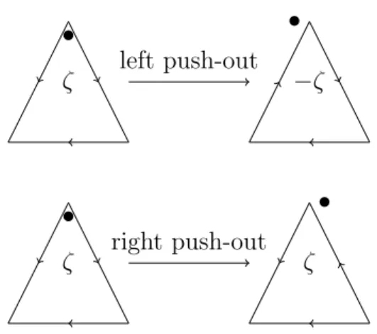
Dans le Chapitre 5 nous exposons certaines propri´et´es de nos coordonn´ees. Chaque choix de triangulation id´eale ⇤ conduit `a un syst`eme de coordonn´ees di↵´erent. Nous montrons alors comment ces coordonn´ees changent lorsqu’on modifie ⇤ par un flip. On obtient alors des lois de transformation semblables `a celles de la Figure 1(cf. Theorem 5.1) qui se r´eduisent aux lois classiques d´ecrites dans la Figure 1.6.
On d´emontre ´egalement que ces changements de coordonn´ees satisfont les relations naturelles d’involution et une super version de la relation du pentagone (cf. Definition 5.2).
Introduction xiii x1 x x4 x3 x2 ⇣ ⇠ x1(1 + x + ⇣⇠px) x 1 x4(1 + x 1+ ⇣⇠ p (x 1)) 1 x 3(1 + x + ⇣⇠px) x2(1 + x 1+ ⇣⇠ p x 1) 1 ⇣px+⇠ p 1+x ⇣ ⇠px p 1+x superflip ! Figure 1 Th´eor`eme (cf. Theorem 5.3).
1. Le superflip est une involution
2. Le superflip satisfait la relation de super pentagone
Dans le Chapitre 6, nous construisons explicitement une structure de Poisson cano-nique sur le super espace de Teichm¨uller de type X. On d´efinit tout d’abord deux op´era-teurs de d´erivations !@
@⇣i et
@
@⇣i (cf. Definition 6.2.1). Nous d´emontrons le r´esultat suivant
en v´erifiant que chaque flip induit une application super-Poisson.
Th´eor`eme (cf. Theorem 6.2.2). L’expression suivante d´efinit une structure de super-Poisson paire sur le super espace de Teichm¨uller de type X :
{, }ST = X i,j2E(⇤•) "ijxixj @ @xi @ @xj 1 2 X k2F (⇤•) @ @⇣k ! @ @⇣k
Encore une fois, ce crochet de Poisson se r´eduit `a celui donn´e dans le cas classique par l’expression (6.1).
Conclusions
Les sujets abord´es dans ce manuscrit s’int`egrent naturellement dans une liste de probl`emes pertinents. Dans notre ´etude, nous construisons un syst`eme de coordonn´ees sur le super espace de Teichm¨uller des super surface de Riemann de dimension (2|1). Une super surface de Riemann de dimension (2|2) peut ˆetre vue comme une classe de conjugaison de morphismes de groupe fondamental dans SpO(2|2). Une premi`ere ´etape dans une ´etude plus approfondie des super espaces de Teichm¨uller serait la construction de coordonn´ees de d´ecalage sur le super espace de Teichm¨uller des super surfaces de Riemann de dimension (2|2) et plus g´en´eralement (2|N).
Une autre direction de recherche pourrait ˆetre l’´etude des super espaces de Teichm¨uller de rang sup´erieur, c’est-`a-dire des espaces de monomorphismes du groupe fondamental d’une surface dans des super groupes qui se r´eduisent en des groupes de Lie classiques comme SL(n,R) par exemple.
Nous aimerions aussi tirer profit du crochet de Poisson que nous avons construit. Il serait sans doute d’une grande utilit´e de d´efinir une quantification du super espace de Teichm¨uller en calquant la construction de la quantification de l’espace de Teichm¨uller classique. De plus notre crochet est pair et la construction d’un crochet de Poisson impair
xiv Introduction sur le super espace de Teichm¨uller, s’il existe, pourrait cr´eer un int´eressant lien avec le formalisme de Batalin-Vilkovisky utilis´e en th´eories de jauge.
Dans notre construction, nous ´etablissons des formules explicites pour les changements de coordonn´ees par application d’un flip. Ces changements pourraient ˆetre vus comme une g´en´eralisation des mutations en th´eorie des vari´et´es amass´ees et nous l’esp´erons con-duiraient `a une version super de ces objets.
Enfin, nous rappelons que notre approche des super espaces de Teichm¨uller est bas´ee sur la d´efinition des supervari´et´es par DeWitt. Une autre d´efinition des supervari´et´es, dite alg´ebro-g´eom´etrique, est bas´ee sur la th´eorie des faisceaux : au lieu de d´eformer la vari´et´e, on d´eforme son alg`ebre de fonctions. Il serait int´eressant de traduire notre travail en ces termes.
English introduction
Context
The problem of the parametrization of complex structures on a given surface dates back to Riemann, who counted the number of parameters of classes of Riemann surfaces up to biholomorphic equivalence. Eighty years later, Teichm¨uller showed that these parameters may be used as real coordinates on a cell, called Teichm¨uller space whose quotient by a natural action of the mapping class group is Riemann’s moduli space.
The Teichm¨uller space, defined in terms of marked surfaces, appeared implicitly in the study of Fuchsian groups by Klein and Poincar´e. The Uniformization theorem of Riemann surfaces due to Klein, Poincar´e and Koebe gives a bijective correspondence be-tween isomorphism classes of Riemann surfaces homeomorphic to Sg and isometry classes
of hyperbolic surfaces homeomorphic to Sg, where Sg is a compact surface of genus g 2.
Using methods based on this theorem, Fricke constructed a system of coordinates on the Teichm¨uller space Tg of Sg and showed that it is a cell of real dimension 6g 6.
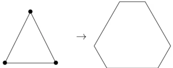
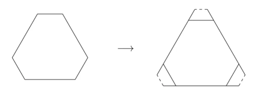
There exist other parametrizations of the Teichm¨uller space and Thurston [32], in the middle of the eighties, showed that each hyperbolic structure on a punctured surface can be described by associating a positive real number to each edge of an ideal triangulation of the surface (i.e. a decomposition of the surface into triangles such that the vertices of the triangulation are exactly the punctures; for an example see Chapter 1, Figure 1.1): these shear parameters encode how to glue together two ideal triangles of the triangu-lation. The shear coordinates have been developed independently by Bonahon [4] and Fock [13] who showed how to express several structures on the Teichm¨uller space through it. The coordinates depend on the ideal triangulation, but changing the triangulation by an elementary move, called flip (cf. Figure 1.2), leads to a change of coordinates which is well controlled. A theorem due independently to Harer [17], Strebel and Penner [28] ensures that each ideal triangulation can be obtained from any other one by applying sequences of these moves, and that these moves satisfy three kinds of relations (involu-tion, distant commutation and most importantly the pentagon relation). In particular the Thurston-Bonahon-Fock-Penner shear coordinates allow to encode the Poisson structure of the Teichm¨uller space in a convenient way and the changes of coordinates preserve the structure. The shear coordinates turned out to be particularly useful to further develop
xvi English introduction the research on the Teichm¨uller space and its higher rank analogues:
1. The quantization of Teichm¨uller spaces was achieved by deforming the algebra gen-erated by the coordinates in the direction of the Poisson structure [6].
2. The study of moduli spaces of representations of the fundamental group of the sur-face in other classical groups as SLn(R) was developed by Fock and Goncharov [12]
who defined coordinates on these moduli spaces (suitably decorated) and estab-lished how the coordinates change while applying a flip. This allowed them to identify combinatorially a “positive” component which corresponds to Hitchin’s. The concept of supermanifold, a generalization of the concept of classical manifold by adding some anticommuting coordinates to the local charts, was introduced by the physicists studying supersymmetry. There exist di↵erent ways to define supermanifolds. We focus in our study on the DeWitt [10] approach, also called the concrete one by Rogers [30, 31]. Roughly, in the DeWitt approach, a supermanifold is a manifold which is locally modeled on a superspace denoted by Rm|n whose coordinates live in super commutative
algebras, called Grassmann algebras (cf. Definition 2.1.2). In particular, this leads to the definition of super Riemann surfaces. In supersymmetric string theory, the super Riemann surfaces are fundamental: they are the worldsheets of the theory. In Polyakov’s formalism (cf. [29, 9]) of bosonic string theory, the computation of the partition function of a string can be performed by integrating over the moduli space of Riemann surfaces. In the supersymmetric approach to string theory, this moduli space should be replaced by its super-analog.
A super Riemann surface can be seen as a conjugacy class of morphisms of its funda-mental group in a group of matrices, with coefficients in the Grassmann algebra, denoted by SpO(2|1). This group projects on SL(2, R) thus one can associate to each super Rie-mann surface its reduction represented by a classical RieRie-mann surface together with a lift of the holonomy from PSL(2,R) to SL(2, R): a spin structure. The super Teichm¨uller space is a super manifold parametrizing the super Riemann surfaces carrying the same topology. This super-Teichm¨uller theory was developed in the case of closed surfaces of genus g [9, 18]. Because of the necessity of a spin structure, the super Teichm¨uller space admits several connected components. Crane and Rabin [9] and Hodgkin [18] showed that each component is a “super ball” of dimension (6g 6|4g 4).
The goal of this thesis is to construct shear coordinates for punctured super Riemann surfaces equipped with an ideal triangulation and define a super Poisson structure on this space using these coordinates. One of the products of these constructions is the computation of the coordinate changes associated to the flips which satisfy all the natural relations, superanalogue of the above listed relations, notably the super pentagons. One of the new features of these coordinates is that in addition to“even” coordinates, on each edge of the triangulation, there are “odd” coordinates for each triangle.
Structure of the work and results
In the first chapter of this thesis, we recall some basic facts about Riemann surfaces and the Teichm¨uller spaces. Let S be an oriented surface of type (g, k, m) i.e a Riemann surface of genus g with two kinds of boundary components : a set of k components called
English introduction xvii holes and a set of m components called punctures. Let H be the Poincar´e half plane and PSL(2,R) its automorphism group. Define the Teichm¨uller space as the space of monomorphisms ⇢ from the fundamental group ⇡1(S) to PSL(2,R) such that the
quo-tient space H/ Im(⇢) is a surface of the same kind as S up to the action of PSL(2, R) by conjugation: we ask that each punture (resp. hole) corresponds to a parabolic (resp. hyperbolic) cusp. We recall Fock’s construction of the shear coordinates on a surface with holes. These coordinates depend on the choice of an ideal triangulation, so a change of triangulation leads to a change of coordinates. We also recall these transformations which are given by the explicit formula (1.2).
In Chapter 2 we recall the definitions and the results about supermanifolds needed in our study. There exists a canonical super-Riemann surface (cf. [15, 9]) generalizing the upper half-plane H, denoted by HS (cf. [9]), and the super analog of the boundary of H
is denoted by P1|1. This super upper half-plane admits a group of transformations (cf.
[15, 9, 5]) which is itself a supermanifold and generalizes the classical group PSL(2,R). It is denoted by SpO(2|1) and it acts on HS and P1|1 by the operation described in (2.3).
Moreover it projects canonically to SL(2,R) and then to PSL(2, R); if is a subgroup of SpO(2|1), one denotes by ] its image by the projection on PSL(2,R). The existence
of these objects leads to the definition of the super-Teichm¨uller space (the group defi-nition by Bryant and Hodgkin [5]) : the super Teichm¨uller space of a surface of type (g, k, m) is the set of monomorphisms : ⇡1(S)! SpO(2|1) such that the quotient space
H/ ( (⇡1(S)))]is a surface of type (g, k, m) modulo the action of SpO(2|1) by conjugation.
The super-Teichm¨uller space of a surface S admits several connected components, in-dexed by the set of spin structures on the surface. Therefore we recall in Chapter 3 the definition of a spin structure on S and di↵erent characterizations of it. We then introduce our key tool in the construction of coordinates on the super-Teichm¨uller space: Kasteleyn orientations on graphs embedded in S. A result of Cimasoni and Reshetikhin [7, 8] states that the set of spin structures on S is in bijection with the set of equivalence classes of Kasteleyn orientations, via a bijection depending on a combinatorial datum called dimer configuration. A spin structure divides the set of punctures on S into those of type Neuveu-Schwarz and those of type Ramond. The component of the super-Teichm¨uller space indexed by has dimension (6g 6 + 3k + 2m|4g 4 + 2k + 2m R ) where R is the number of Ramond punctures for the spin structure .
Chapter 4 is the core of this work. The aim of this chapter is to construct a set of coordinates on the super-Teichm¨uller X-space as follows.
Let S be a surface of type (g, k, m) and denote by p1, . . . , pk the set of holes and by
pk+1, . . . , pk+m the set of punctures.
Definition. The super-Teichm¨uller X space, denoted by ST , is the set of equivalence classes of triples ⇣
⇢,{oi}i=1...k,{Fj}j=1..m
⌘ ,
where ⇢ 2 Hom (⇡1(S), SpO(2|1)) and (Im⇢)] is a Fuchsian group, oi is the choice of
xviii English introduction ⇢(gmk+jg 1) for all g2 ⇡1(S) and mk+j is a simple loop surrounding the puncture pk+jand
where we say that two triples, ⇣⇢,{oi}i=1...k,{Fj}j=1..m
⌘
and ⇣⇢0,{o0
i}i=1...k, Fj0 j=1..m
⌘ , are equivalent if and only if there exists B 2 SpO(2|1) such that
⇢0 = B⇢B 1, o0i = oi and Fj0 = B· Fj.
The choice of fixed points of Ramond punctures increases the dimension of the Te-ichm¨uller space by one odd parameter and each component is isomorphic to a “super ball” of dimension 6g 6 + 3k + 2m|4g 4 + 2k + 2m. We follow the same approach as in the classical case to associate coordinates to an ideal triangulation but we have to handle three main difficulties.
1. We need to encode a spin structure combinatorially : to do so, we use Cimasoni and Reshetikhin’s result about Kasteleyn orientations.
2. The coefficients of the matrices we are dealing with live in a non commutative algebra : this causes that some more care has to be taken when computing.
3. New coordinates of odd type appear, associated to the triangles.
Fix an ideal triangulation ⇤ of S. By associating, as in the classical case, one even coor-dinate x↵ (a super-analog of the cross-ratio) to each edge ↵ of ⇤ and one odd coordinate
⇣i to each face Ti of ⇤, we construct a super-Riemann surface. Hence we get coordinates
which live in RE(⇤)|T (⇤), where E(⇤) and T (⇤) denote respectively the set of edges and
triangles of ⇤. We prove the following:
Theorem (see Theorem 4.3.10). The collection of numbers {x↵, ⇣i} provides a system of
coordinates on the super-Teichm¨uller X-space of S, up to the diagonal action of Z2 by
multiplication of the ⇣i by 1.
In Chapter 5 we give some properties of our coordinates. Each choice of an ideal triangulation ⇤ of the surface leads to a di↵erent system of coordinates. We show how these change when applying a flip on ⇤. We get transformation laws as those in Figure 2 (cf. Theorem 5.1) which reduce to the classical ones described in Figure 1.6.
x1 x x4 x3 x2 ⇣ ⇠ x1(1 + x + ⇣⇠px) x 1 x4(1 + x 1+ ⇣⇠ p (x 1)) 1 x3(1 + x + ⇣⇠px) x2(1 + x 1+ ⇣⇠ p x 1) 1 ⇣px+⇠ p 1+x ⇣ ⇠p px 1+x superflip ! Figure 2
We also show that these coordinate changes satisfy the natural relations of involution and a super version of the pentagon relation (cf. Definition 5.2) :
Theorem (see Theorem 5.3). 1. The superflip is an involution.
English introduction xix 2. The superflip satisfies the superpentagon relation.
In Chapter 6 we construct an explicit canonical Poisson structure on the super-Teichm¨uller X-space. We first define two derivation operators
! @ @⇣i and @ @⇣i (cf. Defini-tion 6.2.1). Then we prove the following by checking that each flip induces a super-Poisson map.
Theorem (see Theorem 6.2.2). The following formula defines an even super Poisson structure on the super Teichm¨uller X space :
{, }ST = X i,j2E(⇤•) "ijxixj @ @xi @ @xj 1 2 X k2F (⇤•) @ @⇣k ! @ @⇣k
and this Poisson bracket does not depend on the particular triangulation.
Once again this Poisson bracket reduces to the classical one given by the formula (6.1).
Conclusions
The topics we dealt with in the present work embed naturally in a list of natural and relevant problems. In our study we construct a system of coordinates on the super Te-ichm¨uller space of super Riemann surfaces of dimension (2|1). A super Riemann surface of dimension (2|2) can be seen as a conjugacy class of morphisms of its fundamental group in SpO(2|2) (cf.[24, 27]). A first step in further investigations would be the construction of shear coordinates on the super Teichm¨uller space of super Riemann surfaces of dimension (2|2) and more generally (2|N).
Another interesting direction of research could be the study of super Teichm¨uller spaces of higher rank, i.e. spaces of monomorphisms of the fundamental group of a surface to super groups which reduce to classical Lie groups, as SL(n,R) for example.
We also would like to make use of our Poisson bracket. It could be useful to define a quantization of the super Teichm¨uller space following the construction of the quantization of the Teichm¨uller space. Moreover our bracket is even and the construction of an odd Poisson bracket on the super Teichm¨uller space, if it exists, could make an interesting link with the Batalin-Vilkovisky formalism used in gauge theories.
In our construction, we establish explicit formulae for a change of coordinates by applying a flip. These changes could be seen as a generalization of the mutations in the theory of cluster varieties and hopefully lead to a super version of these objects.
Finally we recall that our approach to super Teichm¨uller spaces was based on DeWitt’s supermanifold definition. Another definition of supermanifolds uses a sheaf theoretical approach: instead deforming the manifold, one deforms its algebra of functions. It will be interesting to translate our work in these terms.
CHAPTER
1
Teichm¨uller spaces
1.1
The Teichm¨
uller space of Riemann surfaces of
type (g, k, m)
Let S be a connected Hausdor↵ space with a collection {(Vj, zj)}j satisfying the three
following conditions :
1. Every Vj is an open subset of S, and the collection{Vj}j is a cover of S : S =SjVj.
2. Every zj is a homeomorphism of Vj onto an open subset in the complex plane.
3. If Vj \ Vk 6= ;, the transition mapping
zkj := zk zj 1 : zj(Vj\ Vk)! zk(Vj\ Vk)
is a biholomorphism.
Definition 1.1.1. 1. The collection {(Vj, zj)}j is called a system of coordinate
neigh-borhoods on S. We say that this system defines a one-dimensional complex structure on S.
2. A Riemann surface is a connected Hausdor↵ space with a one-dimensional complex structure.
Local analysis on a Riemann surface S is reduced to analysis on domains in the complex plane.
Definition 1.1.2. 1. A holomorphic function on a Riemann surface S is a function f from S to C such that f z 1 is holomorphic on z(V ) for any coordinate
neighbor-hood (V, z) of S.
2 Chapter 1. Teichm¨uller spaces 2. A mapping f of S into a Riemann surface R such that w f z 1 is holomorphic
for all coordinate neighborhoods (V, z) of S and (W, w) of R with f (V )⇢ W is said to be a holomorphic mapping.
3. A holomorphic mapping f : S ! R such that the inverse mapping f 1 : R ! S
exists and is holomorphic, is called a biholomorphic mapping.
Two Riemann surfaces S and R are biholomorphically equivalent if there exists a biholomorphic mapping f : S ! R. We say that S and R have the same complex structure.
We now come to the definition of the Teichm¨uller space. Let S be a closed Riemann surface of genus g 1. The surfaces we are dealing with are endowed with two sets of points called holes and punctures. This distinction will become clear in what follows. We assume that there are k holes and m punctures on S such that 6g 6 + 3k + 2m is positive. We consider triples (S, f, R) where R is a Riemann surface and f : S ! R is an orientation preserving di↵eomorphism. Two triples (S, f1, R1) and (S, f2, R2) are said to
be equivalent if f2 f1 1 is homotopic to the identity.
Definition 1.1.3. The set of all equivalence classes [S, f, R] of triples (S, f, R) is denoted T (S) and is called the Teichm¨uller space based on S.
The Teichm¨uller space may be regarded as the space of complex structures on S mod-ulo the di↵eomorphisms isotopic to the identity. In dimension 2 one can easily establish the equivalence of conformal and complex structures.
Hyperbolic structures and Fuchsian groups
Definition 1.1.4. A hyperbolic structure on S is a complete Riemannian metric of con-stant Gauss curvature 1.
Let H = {z 2 C|=(z) > 0} be the upper half-plane. The uniformization theorem of Klein, Koebe and Poincar´e states that every Riemann surface S of negative Euler charac-teristic is biholomorphic to a certain quotient of the upper half-plane H by a well chosen subgroup of its automorphisms. This theorem gives the equivalence between conformal and hyperbolic structures.
Fuchsian groups. The group of automorphisms of H is the group PSL(2, R). There are three kinds of elements in PSL(2,R) :
1. elliptic elements : they have exactly one fixed point in H ;
2. parabolic elements : they have exactly one fixed point on @H, the boundary of H ; 3. hyperbolic elements : they have exactly two fixed points on @H.
In what follows we will not deal with elliptic elements.
Definition 1.1.5. A Fuchsian group is a discrete subgroup of PSL(2,R) having no elliptic elements. It is called geometrically finite if there exists a convex fundamental region for with finitely many sides.
1.2. Two extensions to open ciliated surfaces 3 In the next section we will look at homomorphisms from the fundamental group of a surface of finite type into PSL(2,R) such that its image is a Fuchsian group. The so obtained Fuchsian group will be finitely generated. We have the following theorem about finitely generated Fuchsian groups.
Theorem 1.1.6. If is a finitely generated Fuchsian group, it is geometrically finite. For a proof of this statement we refer to [22].
The Teichm¨uller-Fricke space. We consider a Riemann surface S of genus g with two sets of marked points. The first is the set of holes and the second the set of punctures. Topologically a neighborhood of such a marked point is an annulus. As a complex surface a neighborhood of a hole is isomorphic to an annulus and a neighborhood of a puncture is isomorphic to a punctured disk. A surface of type (g, k, m) is a Riemann surface of genus g with k holes and m punctures. We denote by Tg,k,m the set of monomorphisms
: ⇡1(S) ! PSL(2, R) such that the quotient H/Im is a surface of type (g, k, m). The
group of automorphisms ofH, PSL(2, R) acts on Tg,k,m by conjugation.
Definition 1.1.7. The space Tg,k,mdefined as the quotient by this action Tg,k,m/PSL(2,R)
is called the Teichm¨uller space based on S.
Theorem 1.1.8. The Teichm¨uller space Tg,k,m is homeomorphic to R6g 6+3k+2m.
For a proof of the theorem in the case of closed surfaces we refer to [20, Chapter 2]. A constructive proof of this is given by Natanzon in [27, p. 28, Theorem 4.1].
1.2
Two extensions to open ciliated surfaces
The definition of the Teichm¨uller space of surfaces was extended by Fock [13] to surfaces with boundary components with some marked points on it. We recall here some of these results which are also exposed in [14].
1.2.1
Ciliated surfaces
Definition 1.2.1. • A ciliated surface is a compact oriented surface with boundary and with a finite set of marked points on the boundary called cilia.
• A boundary component without cilia is either a hole or a puncture.
• A triangulation ⇤ of a ciliated surface is a decomposition of the surface with con-tracted holes into triangles such that every vertex is either a cilium or a concon-tracted hole.
We will make the distinction between the edges of the triangulation belonging to the boundary and the others. The edges of the first kind will be said to be external and the edges of the second kind internal. We denote by T (⇤), E(⇤), E0(⇤), V (⇤) the
sets of triangles, edges, external edges and vertices of the triangulation, respectively. The topology of a ciliated surface is determined by its genus g and a finite collection of integers
4 Chapter 1. Teichm¨uller spaces P = (p1, . . . , ps), where s is the number of boundary components and pi is the number of
cilia on the i th component. We denote by h the number of holes, by c the number of cilia an by n the number of internal edges. Topology gives us the following relations :
1. ]V (⇤) = h + c, 2. ]E0(⇤) = c,
3. ]E(⇤) = 6g 6 + 3s + 2c, 4. n = 6g 6 + 3s + c, 5. ]T (⇤) = 4g 4 + 2s + c.
The topology of the triangulation ⇤ encodes a skew-symmetric matrix of size ]E(⇤), "↵ , where ↵, 2 E(⇤). Consider ↵, 2 E(⇤) and i 2 T (⇤) and define h↵, i, i equals
1 (resp. 1) if ↵ and are sides of the triangle i and ↵ is in the clockwise (resp. counterclockwise) direction from with respect to their common vertex. Otherwise it equals zero. The matrix "↵ is then given by
"↵ = X
i2T (⇤)
h↵, i, i . (1.1) Remark 1.2.2. The entries of the matrix "↵ have values in {0, ±1 ± 2}.
Example 1.2.3. We consider the surface given by g = 1, P = (0). We have the trian-gulation of the Figure 1.1. If we consider the ordered set {↵, , }, corresponding to the edges of the triangulation we have for the matrix
" = 0 @ 02 02 22 2 2 0 1 A .
Figure 1.1: A triangulation of the torus with one contracted hole
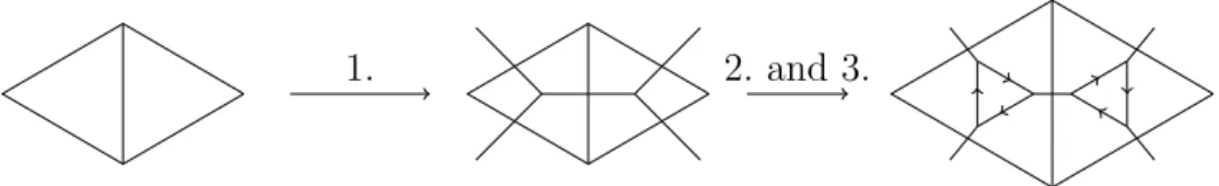
An important result due independently to Strebel, Harer [17] and Penner [28] states that any ideal triangulation can be obtained from another one by a sequence of moves called flips or Whitehead moves (cf. Figure 1.2) and that there are three kinds of relations:
1. The square of a flip is the identity. 2. Flips in disjoint edges commute.
3. Five consecutive flips in edges having one common vertex is the identity (Pentagon relation cf. Figure 1.3).
1.2. Two extensions to open ciliated surfaces 5
Figure 1.2: A flip.
Figure 1.3: Pentagon relation
1.2.2
Teichm¨
uller spaces of surfaces with holes.
The Teichm¨uller X space
In this section we describe a first extension of the Teichm¨uller space to the case of open surfaces. We focus on surfaces of genus g with s boundary components without cilia. Definition 1.2.4. The Teichm¨uller X space of a surface with holes S is the space of com-plex structures on S with an orientation of all holes up to the di↵eomorphisms homotopic to the identity. We denote it byTX(S).
Remark 1.2.5. The Teichm¨uller X space is a 2k-cover of the Teichm¨uller space, where
k denotes the number of holes.
If the surface has several boundary components @1, . . . , @l, l 1, with a non-empty
set of cilia Ci on @i, the definition is more or less the same but special attention has to
be payed to the treatment of these marked points (cf [14]).
We now recall the definition of the Thurston-Bonahon coordinates given by the assign-ment of a positive real number to each internal edge of a triangulation ⇤ of the surface S. This collection of numbers gives a parametrization ofTX(S).
First of all we explain how one can lift the ideal triangulation of S to the upper half plane. We here give the construction introduced by Fock in [13]. We first consider the case
6 Chapter 1. Teichm¨uller spaces where all boundary components are holes. Draw a geodesic around each hole and cut out the arising half cylinders : considering an hyperbolic element 2 PSL(2, R), the quotient H/ < > is a hyperbolic cylinder and the axis of corresponds to a single closed geodesic on the cylinder. We get a surface with geodesic boundary. Cut the surface by the edges of graph of ⇤ into hexagons. Then take an edge and two hexagons sharing this edge and lift the resulting octagon to the upper half plane H. The octagon has four geodesic sides corresponding to the holes. Continue this geodesics to the real axis. The orientations of the holes now induce orientations of the geodesics. Using these orientations we choose one of the two infinities of each geodesic (which correspond to the dot in Figure 1.4). These points of RP1 will be the vertices of the lift of our triangulation. If we have punctures
instead of some holes, some edges of the octagon shrink to a point and no orientation is necessary.
• • • •
Figure 1.4: Lifting of the triangulation
Construction of coordinates After lifting ⇤ to the upper half plane, consider an edge ↵ together with two adjacent ideal triangles forming a quadrilateral. The cross-ratio x, of the four vertices of this quadrilateral is invariant under the action of PSL(2,R). It is convenient to suppose that the coordinates of the ends of the edge ↵ are 0 and 1 and that the coordinate at the third vertex is 1 (cf Figure 1.5). Then the value of the fourth coordinate will be x.
Theorem 1.2.6 (Fock [13]). The collection of positive numbers {x↵}↵2E\E0(⇤) gives a
global parametrization of TX(S) and the orientation of a hole is given by the sign of
Q
x↵ 1, where the product is taken over all the edges ↵ incident to .
To prove the theorem, Fock reconstructs a discrete monodromy group starting from an ideal triangulation of a ciliated surface S with real positive numbers on the internal edges.
Properties of the coordinates If we change the triangulation by a flip in the edge ↵, the coordinates change following the rule given by :
1.2. Two extensions to open ciliated surfaces 7
1 0 x
1
Figure 1.5: The cross-ratio
x00 = 8 > < > : x 1 ↵ if = ↵ x (1 + x↵)" ↵ if "↵ 0 x (1 + (x↵) 1)" ↵ if "↵ 0 (1.2)
If all the edges of the quadrilateral concerned by the flip are di↵erent, the change of coordinate can be summarized in Figure 1.6.
x1 x x4 x3 x2 x1(1 + x) x 1 x4(1 + x 1) 1 x3(1 + x) x2(1 + x 1) 1 Figure 1.6
CHAPTER
2
Supermanifolds
The concept of supermanifolds is a generalization of the concept of classical manifolds including a notion of anticommuting coordinates. There exist di↵erent inequivalent ways to define supermanifolds. Roughly, in the DeWitt approach, a supermanifold is a manifold which is locally modeled on a superspace denoted byRm|n defined in Section 2.1.2. In the algebro-geometric approach, one extends the sheaf of functions on a manifold and not the manifold itself. To study supermanifolds, one replaces the real or complex variables with elements of a super commutative algebra. In this chapter we first recall all the notions of superalgebra needed to define supermanifolds, and then we recall the approaches to supermanifolds. All the ideas developed here can be found in [31, 10, 27].
2.1
Super algebras
2.1.1
Super vector spaces and super commutative algebras
The first concept introduced in the theory of super algebras is that of super vector space, which is a Z2-graded vector space V = V0 V1. The elements of V0 are said to be even
and those of V1 odd. The parity of an homogeneous element v 2 Vi is defined to be|v| = i.
Definition 2.1.1. 1. Let A be an algebra over R or C. Then A is said to be a super algebra if A is a super vector space A = A0 A1 and the multiplication satisfies
AiAj ⇢ Ai+j, where i and j are taken modulo 2.
2. A super algebra A is said to be super commutative if, for all homogeneous elements a and b of A, ab = ( 1)|a||b|ba. In particular the square of an odd element is 0.
For us, the most important examples of super commutative algebras are those of Grassmann algebras used in the definition of (concrete) supermanifolds.
Definition 2.1.2. 1. For each positive integer L, let GL(R) be the real Grassmann
algebra over L generators that is
GL(R) = h1, ↵1, . . . , ↵L|8i, j, 1 i, j L, ↵i = 1.↵i = ↵i.1, ↵i↵j = ↵j↵ii .
10 Chapter 2. Supermanifolds 2. The real Grassmann algebra with infinitely many generators G(R) is defined in the
same way :
G(R) = h1, ↵1, ↵2, . . .|8i, j, ↵i = 1↵i = ↵i1, ↵i↵j = ↵j↵ii .
For p 2 N⇤ [ {1}, let I
p denote the set of all multi indices = 1. . . k with
1 1 · · · k p and including the empty index ;. Set Ip,i, i = 0, 1 the set of
multi indices in Ip which contain a number of indices of parity i.
For L 2 N⇤[ {1}, the super commutative algebra G
L(R) splits in
GL(R) = GL,0(R) GL,1(R),
where, as a vector space,
GL,k(R) = h↵i1. . . ↵in|i = i1. . . in 2 ML,ki
Remark 2.1.3.
1. An element a 2 G(K) is invertible if and only if a] 6= 0.
2. If an element a 2 G(R) is such that a]> 0 then it admits a unique square root pa
determined by (pa)2 = a and (pa)]> 0.
2.1.2
Modules of super algebras and superspaces
In this section, the notion of super module over a super algebra is introduced and the most important example of superspace for the construction of supermanifolds is given. We first recall the definition of homomorphism of super algebras and then conclude by the matrix representation of homomorphisms of free super modules.
Definition 2.1.4. 1. Let V and W be two super vector spaces. If f is a linear map of V to W , then f is said to be a super vector space homomorphism.
2. A super vector space homomorphism f is said to be even (resp. odd ) if for all v 2 V , |f(v)| = |v| mod 2 (resp. |f(v)| = |v| + 1) and the parity of f is denoted by |f|. 3. Let A and B be super algebras overR or C. Let f : A ! B be a super vector space
homomorphism of a given parity, then f is said to be a super algebra homomorphism if
8a1, a2 2 A, f(a1a2) = ( 1)|f||a1|f (a1)f (a2).
The definition of super modules is analogous to the definition of a classical module, but a compatibility of the parities is required.
Definition 2.1.5. 1. Let V = V0 V1 be a super vector space and A a super
com-mutative algebra. Then V is said to be a left super A-module if there exists a map
A⇥ V ! V (a, v)7! av
2.1. Super algebras 11 such that 8(a1, a2)2 A2,8v 2 V, ⇢ |a1v| = |a1| + |v| a1(a2v) = (a1a2)v .
2. Assume that there exist n elements B1, . . . , Bnof V0and m elements Bn+1, . . . , Bn+m
of V1 such that each element v2 V can be decomposed uniquely in
v =
n+mX i=1
aiBi,
for ai 2 A. In this case V is said to be a free super A-module of dimension (n, m),
and the set {B1, . . . , Bn+m} is said to be a (n, m) super basis.
Remark 2.1.6. If v is even then it may be expressed as (a1, . . . , an+m) which is an element
of the superspace corresponding to A, An|m, defined as
An|m= (A0)n⇥ (A1)m.
The superspace which plays a particular role in the concrete construction of superman-ifolds is the (n|m)-dimensional superspace corresponding to GL(R), where L 2 N⇤[ {1},
denoted by
Rn|m
L = (GL,0(R))n⇥ (GL,1(R))m.
An element ofRn|mL will be denoted by (x|⇣) = (x1, . . . , xn|⇣1, . . . , ⇣m).
Definition 2.1.7. Let A be a super commutative algebra and let V and W be two super A-modules. Then a map f : V ! W is said to be a homomorphism of super A-modules if f is a super vector space homomorphism and
8a 2 A, 8v 2 V, f(av) = ( 1)|a||f|af (v).
Even homomorphisms of super A-modules (in terms of particular bases) can be rep-resented by super matrices.
Definition 2.1.8. A (p, q)⇥ (r, s) super matrix over a super commutative algebra A is a (p + q)⇥ (r + s) matrix M whose entries are elements of A, and which can be represented by blocks M = r columns s columns ✓ ◆ M0,0 M0,1 p lines M1,0 M1,1 q lines
where the entries of Mi,j are elements of Ai+j.
The sum and the product of super matrices are defined in the same way as in the classical case, but with the requirement that the resulting matrices always are super matrices.
12 Chapter 2. Supermanifolds
2.2
Supersmooth functions on
R
n|mIn this section we are interested in the particular case where the super commutative alge-bra A is a Grassmann algealge-bra. We focus more specifically to G(R) and its corresponding superspace Rn|m. The most important topology on Rn|m (L is infinite) is the DeWitt
topology and it will now be defined. The super space Rn|m plays the role of Rn in the
definition of supermanifolds, we then need functions which play the role of C1 functions.
2.2.1
The DeWitt topology
Let x be an element of GL(R) for L 2 N⇤[{1}. There is a unique algebra homomorphism
] : GL(R) ! R which sends 1 to 1 and for all i, ↵i to 0; the image ](x) = x] is called the
reduction of x. The map ] can be extended to RnL|m by ]n|m :RnL|m ! Rn
(x1, . . . , xn|⇣1, . . . , ⇣m)7 ! (x]1, . . . , x]n).
The image (x]1, . . . , x]
n) of an element ofRn|mL will be called its reduction.
Definition 2.2.1. A subset U ⇢ Rn|m is said to be open in the DeWitt topology if and
only if there exists an open subset V of Rn such that U = ]n|m 1(V ).
Remark 2.2.2. The DeWitt topology is not Hausdor↵.
2.2.2
Supersmooth functions on
R
n|mThe Grassmann analytic continuation is the key in the definition of supersmooth functions. For each positive integer L let pL : G(R) ! GL(R) be the projection which sends the
generators ↵i of G(R) to 0 for i > L.
Definition 2.2.3. Let V ⇢ Rn be open and let f : V ! G(R).
1. The function f is said to be of class C1 if for each positive integer L the function
pL f : V ! GL(R) is C1. The set of these functions is denoted by C1(V, G(R)).
2. If f belongs toC1(V, G(R)) then define the function bf : (]n|0) 1(V )! G(R) by
b f (x) = 1 X i1=0,...,in=0 1 i1! . . . in! @i1 1 . . . @ninf (]n|m(x))s(x1)i1. . . s(xn)in.
Definition 2.2.4. Let U ⇢ Rn|m be open. The function f : U ! G(R) is said to be of
class G1 if and only if there exists a collection {f | 2 Im, f 2 C1(]n|m(U ), G(R))} such
that
8(x, ⇣) 2 U, f(x|⇣) = X
2Im
b f (x)⇣ .
2.3. The definition of DeWitt supermanifolds 13 A more restricted class of supersmooth functions which makes the link between the two approaches to supermanifolds can be defined.
Definition 2.2.5. Let U ⇢ Rn|m be open. The function f : U ! G(R) is said to be of
class H1 if and only if there exists a collection {f | 2 Im, f 2 C1(]n|m(U ),R)} such
that
8(x, ⇣) 2 U, f(x|⇣) = X
2Im
b f (x)⇣ .
Remark 2.2.6. 1. The di↵erence between the two definitions lies in the fact that in the case of G1-functions, the functions f take their values in G(R) and in the case
of H1-functions, it is in R.
2. Any H1-function is also a G1-function, but the converse is not true.
2.3
The definition of DeWitt supermanifolds
The construction of DeWitt supermanifolds is analogous to the construction of manifolds. The DeWitt supermanifolds are modeled on the superspaceRn|m and the transition
func-tions will be supersmooth funcfunc-tions of a given class K, where K = G1 or H1. Definition 2.3.1. Let M be a set, and n and m two positive integers.
1. An (n|m) K chart on M is a pair (V, '), where V is a subset of M and ' is a bijective map from V to U ⇢ Rn|m, U open for the DeWitt topology.
2. An (n|m) K atlas on M is a collection of charts {(Vj, 'j)|j 2 J} such that
(a) [
j2J
Vj = M
(b) for i, j 2 J such that Vi\ Vj 6= ;,the sets 'i(Vi\ Vj) and 'j(Vi\ Vj) are open
and the map
'j 'i 1 : 'i(Vi\ Vj)! 'j(Vi \ Vj)
is of class K.
3. An (n|m) K DeWitt super-premanifold is a set M together with a maximal (n|m) K atlas on M .
Two standard examples will now be given.
Example 2.3.2. The superspace Rn|m can be endowed with the structure of G1 or H1 super-premanifold. Indeed (Rn|m, Id) is a (n|m) chart on Rn|m and {(Rn|m, Id)} is an
(n|m) atlas on M.
Example 2.3.3. In the same way if V is an open subset of R(n|m), then (V, ı) (where
ı : V ,! R(n|m) is the inclusion) is an (n|m) chart on V and {(V, ı)} is an (n|m) atlas on
14 Chapter 2. Supermanifolds
2.3.1
The topology of a DeWitt super-premanifold
The structure of super-premanifold gives a natural way to define a topology on M . Indeed, if M is a (n|m) K DeWitt super-premanifold together with a maximal atlas {(Vj, 'j)|j 2
J}, let ⌧DeWitt be the collection of subsets U ⇢ M such that 8j 2 J, 'j(U\ Vj) is open in
Rn|m. Then ⌧
DeWitt is a (non-Hausdor↵) topology on M . This construction is analogous
to the construction in the case of classical manifolds.
2.3.2
The body of a DeWitt super-premanifold
A DeWitt super-premanifold has a naturally underlying classical topological space of dimension n. We recall the construction due to DeWitt [10] and Batchelor [2] of this space in the following theorem.
Theorem 2.3.4. Let M be a (n|m) K DeWitt super-premanifold (with the DeWitt topology). Let {(Vj, 'j)|j 2 J}. Then the following holds.
1. the relation ⇠ generated on M by
(p⇠ q) , 9j 2 J| p, q 2 Vj and ]n|m('j(p)) = ]n|m('j(q))
is an equivalence relation.
2. The space M] = M/ ⇠ is locally di↵eomorphic to Rn, with atlas {(V] j, ' ] j)|j 2 J},where Vj] ={[p], p 2 Vj} ']j : Vj] ! Rn [p] 7! ]n|m ' j(p).
Definition 2.3.5. The space M/ ⇠ is called the body of M and denoted M]. The
canonical projection of M to M] is denoted by ].
Definition 2.3.6. A DeWitt supermanifold is a super-premanifold M whose body M] is
a classical manifold.
In what follows we only consider supermanifolds.
2.3.3
The algebro-geometric approach to supermanifolds
In the algebro-geometric approach it is not the manifold which is extended but a sheaf of functions. Here we just recall the definition of supermanifold which was given by Le˘ıtes [23], and conclude by recalling the link between algebro-geometric and H1-DeWitt
supermanifolds. We will say no more about this approach because, in what follows, we are only interested in the concrete one. Our results are based on the theory developed in Natanzon’s book [27] which uses the DeWitt approach to supermanifolds.
Definition 2.3.7. A smooth real algebro-geometric supermanifold of dimension (n|m) is a pair (M, A) where M is a real n dimensional manifold and A is a sheaf of super commutative algebras over M such that
2.4. Further examples 15 1. there exists an open cover of M , {(Uj, 'j)|j 2 J} where
8j 2 J, A(Uj) ⇠= C1(Uj)⌦ ⇤(Rm),
2. if N is the sheaf of nilpotents in A, then (M, A/N ) is isomorphic to (M, C1).
The link between the two approaches
Rogers [31] showed the existence of a unique algebro-geometric supermanifold correspond-ing to a given H1 DeWitt supermanifold.
Theorem 2.3.8. Let M be an H1 DeWitt supermanifold of dimension (n|m), and let A
be the sheaf of super algebras on M] given by A(V ) = H1(] 1(V )). Then M], A is an
algebro-geometric supermanifold of dimension (n|m).
Conversely, starting with an algebro-geometric super manifold (X, A), one can con-struct a DeWitt supermanifold M (X, A) such that M (X, A)] is X and the algebro-geometric supermanifold corresponding to the sheaf of H1 functions on M (X, A) is
iso-morphic to (X, A). Batchelor [3] shows that the so constructed correspondence between the two approaches is bijective.
2.4
Further examples
2.4.1
Real super projective spaces
Let (Rn+1|m)⇤ ⇢ Rn+1|mbe the set (]n+1|m) 1(Rn+1 {0}). Two elements (x|⇣) and (x0|⇣0)
of (Rn+1|m)⇤ are said to be equivalent if there exists an invertible element `2 G
0(R) such
that
xi = `x0i i = 1, . . . , n + 1
⇣j = `⇣j0 j = 1, . . . , m.
Let ⇠ denote the equivalence relation defined above and let [(x, ⇣)] denote the class of (x, ⇣). ThenPn|m= (Rn+1|m)⇤/⇠ can be endowed with a structure of DeWitt
superman-ifold by defining the following atlas. For all i = 1, . . . , n + 1 let Vi = n [(x|⇣)], (x|⇣) 2 (Rn+1|m)⇤, x]i 6= 0o 'i : Vi ! R(n|m) [(x|⇣)] 7! ✓ x1 xi , . . . ,cxi xi , . . . ,xn+1 xi ⇣1 xi , . . . ,⇣m xi ◆ .
16 Chapter 2. Supermanifolds
2.4.2
The super upper half-plane
Before developing this example we just stress that all the definitions we recall about real Grassmann algebras and real superspaces can be given in an analogous way in the complex case. A complex DeWitt supermanifold will be modeled on Cn|m and the transition
functions will be superholomorphic.
Definition 2.4.1. Let U ⇢ Cn|m be open. The function f : U ! G(C) is said to be
superholomorphic if and only if there exists a collection {f | 2 Mm} of functions taking
their values in G(C) and being holomorphic on ]n|m(U ) such that
8(z, ⇣) 2 U, f(z|⇣) = X
2Mm
ˆ f (z)⇣ .
The so obtained function on U is called the Grassmann analytic continuation of f . The space HS will play the role of the upper-half plane H. It is defined by
HS ={(z|⇣) 2 C(1|1);=(z]) > 0},
where =(z]) denotes the imaginary part of z]. As in the classical case, there exists a
notion of boundary of HS which can be seen as the union ofR1|1 and of points at infinity.
Definition 2.4.2. The boundary of HS is defined to beP1|1
As in the classical case, P1|1 admits a covering with two charts. We will often use the following notation: given Z 2 P1|1, choose a representative of Z inR2|1⇤, say ˆZ =
0 @ zz12 ⌘ 1 A and set z = z1 z2, ' = ⌘ z2. We then write Z as ✓ z ' ◆ . Notation. If a representative 0 @ zz12 ⌘ 1
A of an element Z 2 P1|1is such that z
2 is not
invert-ible, then Z lies in the second chart of P1|1. In the special case where the representative has the form
0 @ x0 ⇣ 1 A, Z will be denoted by ✓ 1 ⇣ x ◆ .
2.4.3
The group SpO(2
|1)(R)
Consider first a matrix with coefficient in G(K), M = ✓
A B C D
◆
, represented by blocks, where A and D are respectively of size 2⇥ 2 and 1 ⇥ 1 and have even entries, and, B and C have odd ones. Such a matrix is said to be even.
Definition 2.4.3. The supertranspose (cf. [25]) of a matrix is given by ✓ A B C D ◆st = ✓ At Ct Bt Dt ◆ .
2.4. Further examples 17 Definition 2.4.4. The superdeterminant or Berezinian (cf. [25]) of M is defined if and only if M is square, A and D are invertible and we have
Ber M = det(A BD 1C) det(D) 1. Definition and properties
Definition 2.4.5. The group SpO(2|1) is the group of all square even matrices B, with Ber(B) = 1, which satisfy the relation
Bst 0 @ 01 01 00 0 0 1 1 A B = 0 @ 01 01 00 0 0 1 1 A . (2.1)
An element B in SpO(2|1) is a matrix of the form B = 0 @ a bc d ↵ e 1 A, where 8 > > > > > > < > > > > > > : a, b, c, d, e2 G0(R), ↵, , , 2 G1(R), ad bc ↵ = e2+ 2 = 1, a c e↵ = b d e = 0, Ber(B) = 1. (2.2)
These relations are equivalent to (2.1). The group SpO(2|1) is the group of automorphism of HS (cf. [5]).
One defines an epimorphism ] from SpO(2|1) to PSL(2, R) sending B = 0 @ a bc d ↵ e 1 A to ](B) = z7! B](z) = a]z+b] c]z+d].
Definition 2.4.6. The homography ](B) is called the reduction of B.
The action of B = 0 @ a bc d
↵ e 1
A on HS and on P1|1 is given by B· Z = Z0, where :
z0 = az + b + '
cz + d + ' , '
0 = ↵z + + e'
cz + d + '. (2.3) Lemma 2.4.7. 1. For any triple
✓ z1 ✓1 ◆ , ✓ z2 ✓2 ◆ , ✓ z3 ✓3 ◆
inP1|1 with distinct bodies,
there exists an element B 2 PSL(2, R) such that B· ✓ z1 ✓1 ◆ = ✓ 1 0 ◆ , B· ✓ z2 ✓2 ◆ = ✓ 1 ✓ ◆ , B· ✓ z3 ✓3 ◆ = ✓ 0 0 ◆ .