Surface tension and capillary waves at the nematic-isotropic interface in ternary mixtures of liquid crystal, colloids, and impurities

HAL Id: ensl-00182728

https://hal-ens-lyon.archives-ouvertes.fr/ensl-00182728

Submitted on 26 Oct 2007

HAL is a multi-disciplinary open access

archive for the deposit and dissemination of

sci-entific research documents, whether they are

pub-lished or not. The documents may come from

teaching and research institutions in France or

abroad, or from public or private research centers.

L’archive ouverte pluridisciplinaire HAL, est

destinée au dépôt et à la diffusion de documents

scientifiques de niveau recherche, publiés ou non,

émanant des établissements d’enseignement et de

recherche français ou étrangers, des laboratoires

publics ou privés.

nematic-isotropic interface in ternary mixtures of liquid

crystal, colloids, and impurities

Vlad Popa Nita, Patrick Oswald

To cite this version:

Vlad Popa Nita, Patrick Oswald. Surface tension and capillary waves at the nematic-isotropic interface

in ternary mixtures of liquid crystal, colloids, and impurities. Journal of Chemical Physics, American

Institute of Physics, 2007, 127 (10), pp.104702. �ensl-00182728�

Surface tension and capillary waves at the nematic-isotropic interface

in ternary mixtures of liquid crystal, colloids, and impurities

V. Popa-Nitaa兲

Faculty of Physics, University of Bucharest, P.O. Box MG-11, Bucharest 077125, Romania P. Oswald

Laboratoire de Physique de l’Ecole Normale Supérieure de Lyon, 46 Allée d’Italie, 69364 Lyon Cedex 07, France

共Received 14 May 2007; accepted 21 July 2007; published online 12 September 2007兲

In mixtures of thermotropic liquid crystals with spherical poly共methyl methacrylate兲 particles, self-supporting networklike structures are formed during slow cooling past the isotropic-to-nematic phase transition. Experimental results support the hypothesis that a third component, alkane remnants slowly liberated from the particles, plays a crucial role. A theoretical model, based on the phenomenological Landau–de Gennes, Carnahan-Starling, and hard-sphere crystal theories, is developed to describe the continuous phase separation in a ternary nematic-impurity-colloid mixture. The interfacial tension and the dispersion relation of the surface modes of the nematic-isotropic interface are determined. The colloids decrease the interfacial tension and the damping rate of surface waves, whereas impurities act in an opposite way. This should strongly influence the formation of abovementioned networklike structures and could help explain some of their rheological properties. © 2007 American Institute of Physics.关DOI:10.1063/1.2772251兴 I. INTRODUCTION

Recently, there has been a considerable interest in col-loidal particles dispersed in anisotropic media, principally liquid crystals.1–6When particles are immersed in a nematic liquid crystal, the director field is distorted by the particles, generating interesting new phenomena. Depending on the type of anchoring共planar or homeotropic兲 and on its penetra-tion length Lp= K / W共with K the Frank elastic constant and

W the anchoring energy of the nematic at the particle surface7,8兲, different structures develop around a single par-ticle. For instance, for homeotropic anchoring a point defect 共“hedgehog”兲 or a “Saturn ring” can nucleate nearby the par-ticle depending on whether Lpis small共strong anchoring兲 or

large共weak anchoring兲 with respect to R 共for a review about this problem, see Ref. 6兲. These defects give rise to highly

anisotropic, long-range elastic interactions of dipolar or qua-drupolar type between the dispersed particles.

These induced interactions lead to original patterns, such as chaining which is the most commonly observed at low concentration of particles.9–11

The situation becomes different at large concentration of particles because the latter tends to separate from the nematic phase to form an isotropic phase共liquid or solid兲 which co-exists with the nematic phase. This separation is due共only in part, as we shall see later兲 to the distortions of the director field cost energy.12–17 It turns out that the first studies have focused on dispersions of⬇200 nm size poly共methyl meth-acrylate兲 共PMMA兲 spheres in 4

⬘

-pentyl-4-cyanobiphenyl 共5CB兲 or N-4-methoxybenzylidene-4

⬘

-butylaniline. Micro-scopic observations have shown that below the

nematic-to-isotropic phase transition temperature, the two phases coexist by forming a three-dimensional network which gives to the mixture the consistency of a soft cellular solid. More pre-cisely, the particles are densely packed in relatively thin walls constituting the isotropic phase, while the cavities in between are filled with almost pure nematic liquid crystal.

In these experiments, the network was formed in the weak-anchoring limit as the particle radius was very small 共RⰆLp兲. This condition is nevertheless not crucial because

similar networks were recently observed in the opposite strong-anchoring limit by using micrometer-sized particles for which RⰇLp.16–18These studies showed, in addition, that

experiments共including those reported before in Refs.12–15兲

were not dealing with binary but with ternary systems. The reason is that during the process of particle preparation, the remnant alkane cannot be removed completely. As a conse-quence, it slowly diffuses into the suspension after homog-enization. This phenomenon may be important, firstly, be-cause the particles are wetted by a layer of alkane which can change the anchoring of the liquid crystal molecules on their surfaces. Secondly, the nematic-to-isotropic transition tem-perature is lowered while a biphasic region shows up in the presence of alkane, favoring the formation of the cellular structure. It is this second point that we propose to study theoretically.

More precisely, we shall first develop a model based on the Landau–de Gennes mean field treatment to determine the phase diagram of a ternary system consisting of a nematic liquid crystal, impurities共a non-nematogenic fluid兲, and col-loids. We will see that in this mixture, a biphasic region between the isotropic and the nematic phases appears below the nematic-to-isotropic transition temperature of the pure liquid crystal. We shall then study the static and dynamic

a兲_{Author to whom correspondence should be addressed. Electronic mail:}

[email protected]

THE JOURNAL OF CHEMICAL PHYSICS 127, 104702共2007兲

properties of the nematic-isotropic interface共more precisely, its surface tension and its capillary waves兲. As we have al-ready treated this problem in the particular case of a binary mixture of liquid crystal and nonmesogenic impurities 共see the previous article19兲, we shall mainly focus our attention on the influence of added colloids on the properties of the nematic-isotropic interface.

The paper is organized as follows. In Sec. II, we intro-duce the free energy of a nonuniform ternary liquid crystal– impurity–colloid mixture. In Sec. III, we present the binary 共without colloids兲 and ternary phase diagrams. In Sec. IV, a general expression for the nematic-isotropic surface tension is derived. This quantity is then calculated explicitly for typi-cal values of the parameters. Its large variations as a function of the colloid and the impurity concentrations are empha-sized and are discussed in the framework of the experiments reported before. In Sec. V, we give the dynamical governing equations necessary to calculate the dispersion relation for capillary waves at the nematic-isotropic interface. Numerical results about the damping rate of the waves are then pre-sented and discussed. Finally, in Sec. VI, we draw some conclusions and directions for future work.

II. FREE ENERGY

The mixture is characterized by the volume fractions of the three components,

⌽i= Nivi ⌺i=13 Nivi with

兺

i=1 3 ⌽i= 1, 共1兲

where Ni is the number of molecules of component i 共i=1

defines the liquid crystal, i = 2 the non-nematogenic fluid, and i = 3 the colloids兲 and viis the volume of a particle of

com-ponent i. In what follows, we consider that the volumes of a nematic and impurity molecule are equal共v₁=v₂=v兲 and the volume of a colloid isvR=共4␲/ 3兲R3, where R is the radius of

a colloid particle共with vRⰇv兲. The orientational order of the

mixture is characterized by the nematic order parameter Q_␣␤ 共with Cartesian indices ␣, ␤= 1 , 2 , 3兲 which, in the case of uniaxial nematic state, can be expressed as7

Q_␣␤= S共3n_␣n_␤−␦_␣␤兲/2. 共2兲

The unit vector n is the nematic director which fixes the average local uniaxial orientation of the liquid crystal mol-ecules. Due to the head-to-tail invariance of molecules, the cases ±n refer to the same state. The scalar S is the orienta-tional order parameter. The isotropic liquid is characterized by S = 0 and a perfectly oriented nematic phase共i.e., with no fluctuations about n兲 would correspond to S=1. In this paper, we suppose to simplify that n is fixed in space and time, so that the relevant physics is only governed by the scalar order parameter S共r,t兲. We note that this is an idealization which is neither true in general during the relaxation nor close to the interface even at equilibrium. However, previous studies20 suggest that the slowest relaxation modes approximately ful-fill this condition when the director anchoring is homeotropic at the interface.

The free energy functional of the system is given by

F关⌽₁,⌽₂,⌽₃,Q_␣␤兴 =

冕

冋

f共⌽₁,⌽₂,⌽₃,Q_␣␤兲 +1 2K⌽共ⵜ⌽2兲 2₊1 2L1共⳵␥Q␣␤兲 2 +1 2L2共⳵␣Q␣␤兲 2

册

_{dV, 共3兲}

where K_⌽is a phenomenological coefficient. The elastic con-stants L1 and L2are related to the Frank-Oseen elastic

con-stants by the relations K₁= K₃= 9S_n2共L₁+ L₂/ 2兲/2 and K₂ = 9Sn2L1/ 2, where Snis the bulk nematic order parameter. In

the so-called “one-constant approximation” 共K1= K2= K3

= 9Sn2KS/ 2兲, L1= KS and L2= 0, values which we consider in

this paper. We neglect contributions from a gradient in the colloid concentration. The reason is that the contribution of colloids to the total interfacial tension is negligibly small due to the large size of the particles 共indeed, it scales as the thermal energy divided by the size of the particle squared兲. Since the colloids are at least ten and more likely 100 times larger than the molecules of liquid crystal, their contribution is insignificant. The interfacial tension between phase-separated colloidal phases can be as low as a few millionth of a N/m.21 We have also neglected the coupling term K0共⳵␣⌽2兲共⳵␤Q␣␤兲, since previous study indicates that its

in-fluence to interfacial tension is small.19

The bulk free energy density consists of three parts,

f共⌽1,⌽2,⌽3,Q␣␤兲 = fmix共⌽1,⌽2兲 + fcoll共⌽3兲

+ flc共⌽1,⌽2,⌽3,Q␣␤兲. 共4兲

The first term is the free energy density of the isotropic mixing of liquid crystal and non-nematic fluid and according to the Flory theory is given by22

fmix=

kBT

v 共⌽1ln⌽1+⌽2ln⌽2+␹⌽1⌽2兲, 共5兲

where kBis the Boltzmann constant, T the absolute

tempera-ture, and␹=␹12the dimensionless Flory-Huggins interaction

parameter which characterizes the isotropic interaction en-ergy共divided by kBT兲 between the liquid crystal and impurity

molecules.22In this paper, we consider ␹ as a constant. Be-cause vRⰇv, the interaction between the colloidal particles

and the liquid crystal and impurity molecules can be ne-glected 关␹₁₃=␹₂₃= 0 as these two quantities are of the order of 共v/vR兲1/3␹Ⰶ␹兴.

The second term in Eq.共4兲is the free energy density of a colloidal suspension,

f_coll=kBT vR

再

⌽3ln⌽3+⌽3 2_{共4 − 3⌽} 3兲/共1 − ⌽3兲2, ⌽3⬍ 0.52, liquid u0⌽3+ 3⌽3ln⌽3/共1 − ⌽3/⌽c兲, ⌽3⬎ 0.52, solid,

冎

共6兲

where the two expressions are matched by the adjustable parameter u0= 1.793 at the concentration of 0.52, while ⌽c

= 0.637 is the random close-packing fraction. The first line in Eq.共6兲is the Carnahan-Starling excess free energy density of a hard-sphere suspension,23while the second line is the free energy density of a hard-sphere crystal based on free volume considerations.24

The third term in Eq.共4兲 is the Landau–de Gennes free energy density,7 which describes the weakly first-order nematic-to-isotropic phase transition,

flc=⌽1关a共T − 共1 − ␭2⌽2−␭3⌽3兲T*兲Q␣␤Q␤␣

− BQ_␣␤Q_␤␥Q_␥␣+ C共Q_␣␤Q_␤␣兲2兴. 共7兲 In this expression, T*_{is the spinodal temperature of the}

iso-tropic phase of the pure liquid crystal, and a, B, and C are three constant coefficients. For 5CB for instance, they have the following values: a⬇3.5⫻104J / m3K, B⬇7.1 ⫻105_{J / m}3_{, and C⬇4.3⫻10}5_{J / m}3_.8,25

We shall take these values in the following. The term 共1−␭2⌽2−␭3⌽3兲T*

en-sures that the nematic-to-isotropic transition temperature de-creases linearly as a function of the impurity and colloid concentrations. The physical origin of the coupling param-eters␭2and␭3is discussed in Refs.19and14, respectively.

In this paper, we consider them as phenomenological param-eters.

For the pure liquid crystal共⌽1= 1 and⌽2=⌽3= 0兲, using

the form of Eq.共2兲for Q_␣␤, the bulk free energy density has the well-known expression,

flc= 3 2a共T − T *_兲S2₋3 4BS 3₊9 4CS 4_{. 共8兲}

This equation describes a weakly first-order nematic-to-isotropic phase transition. At T = T_NI= T*_{+ B}2_{/ 24aC, the two}

phases, nematic共S_{nem 0}= B / 6C兲 and isotropic 共S_iso= 0兲, coex-ist in equilibrium.

III. PHASE DIAGRAMS

A. Basic equations for calculating phase diagrams

The calculation of the static phase diagrams only re-quires to know the bulk free energy density. For conve-nience, we introduce nondimensional quantities. The tem-perature is replaced by the reduced temperature ␶ =共T−T*_兲/共T

NI− T*兲. The orientational order parameter is

normalized with respect to its value in the pure liquid crystal at the transition temperature T_NI: S¯ =S/S_{nem 0}. Setting f¯_coll = fcoll/共kBT /vR兲 and ␭¯2,3= 24aT*C␭2,3/ B2, the dimensionless

free energy f¯ = f / f0共with f0= B4/ 242C3兲 reads after omitting

the bar notation,

f =⌫共1 +␦␶兲共⌽1ln⌽1+⌽2ln⌽2+␹⌽1⌽2兲

+⌫R共1 +␦␶兲fcoll+⌽1关共␶+␭2⌽2+␭3⌽3兲S2− 2S3+ S4兴,

共9兲 where⌫=kBT*/共vf0兲, ⌫R= kBT*/共vRf0兲, and␦=共TNI− T*兲/T*.

Below TNI, a phase separation may occur depending on

the initial composition of the mixture. During this process, the system of average composition 共⌽2,⌽3兲 splits into a

nematic phase of composition共⌽2nem,⌽3nem兲 and an

isotro-pic phase of composition共⌽_2iso,⌽_3iso兲. The values of ⌽_2nem, ⌽3nem,⌽2iso, and⌽3isoare given at equilibrium by the

equa-tions共remembering that ⌽₁= 1 −⌽₂−⌽₃ in each phase兲

␮2⬅␮2共Snem,⌽2nem,⌽3nem兲 =␮2共0,⌽2iso,⌽3iso兲,

␮3⬅␮3共Snem,⌽2nem,⌽3nem兲 =␮3共0,⌽2iso,⌽3iso兲, 共10兲

g⬅ g共S_nem,⌽_2nem,⌽_3nem兲 = g共0,⌽_2iso,⌽_3iso兲,

where␮2共S,⌽2,⌽3兲,␮3共S,⌽2,⌽3兲, and g共S,⌽2,⌽3兲 are

de-fined by the equations

␮2共S,⌽2,⌽3兲 = ⳵f ⳵⌽2 ; ␮3共S,⌽2,⌽3兲 = ⳵f ⳵⌽3 ; 共11兲 g共S,⌽₂,⌽₃兲 = f −␮₂⌽₂−␮₃⌽₃.

We emphasize that in the definition of grand potential g共S,⌽2,⌽3兲,␮2 and␮3 are the constant chemical potentials

of the impurities and of the colloids, respectively. As for the orientational order parameter Snem, it is obtained by

minimiz-ing the free energy density关Eq.共9兲兴 with respect to S, which gives

Snem= 1

4共3 +

冑

9 − 8共␭2⌽2+␭3⌽3+␶兲兲, 共12兲

while Siso= 0. Note that, with our new notations, Snem 0= 1 in

the pure liquid crystal共⌽2=⌽3= 0兲 at␶= 1. In the following,

we discuss separately the cases of the binary and ternary diagrams.

B. Binary phase diagram of the liquid crystal–impurity mixture

This case corresponds to⌽3= 0. To simplify, we denote

by ⌽ the average impurity volume fraction ⌽2 and by

1 −⌽ the liquid crystal volume fraction ⌽1. To compute the

phase diagram, we must choose a value for ⌫. This param-eter depends on f0, the value of the energy barrier to

over-come at the nematic-to-isotropic phase transition in the pure liquid crystal. From typical values of a, B, and C given above for 5CB, we calculate f0⬇5500 J/m3. Volumev

rep-resents in an ideal mixture the molecular volume. In the case of liquid crystal 5CB, each molecule has the shape of a cyl-inder of length of 3 nm and of diameter of 0.5 nm. That

gives v⬇22.5⫻10−27_m3_{. From this value, we calculate ⌫}

⬇300. It turns out that if we perform the calculations with this value of⌫, we do not find any phase separation at the nematic-to-isotropic phase transition.

On the other hand, choosing a smaller value of⌫ allows us to find a phase diagram compatible with observations.26 Such a phase diagram, calculated for ⌫=0.8, ␭2= 1, and ␹

= 1, is shown in Fig.1. Consequently, we must decrease the value of⌫ by more than two orders of magnitude to obtain an acceptable phase diagram. That means that the mixing entropy of the liquid crystal and impurity molecules is smaller than expected. This is possible if molecules of each species form clusters. Sov must be considered as an effec-tive volume共larger than the molecular volume兲 characteriz-ing the nonideality of the mixture. In the followcharacteriz-ing, we shall retain the phenomenological value⌫=0.8.

We now briefly describe the obtained phase diagram. For a temperature below T_NI 共␶_NI= 1兲, there exists a two-phase coexistence region between an isotropic共high-⌽兲 and a nem-atic共low-⌽兲 phase. On decreasing temperature 共note that the spinodal temperature of the isotropic phase of the pure liquid crystal corresponds to ␶*_{= 0兲, the biphasic region broadens.}

When the system is thermally quenched from the stable iso-tropic phase into the biphasic region, fluctuations of the con-centration and of the orientational order occur, and nematic droplets nucleate. At the end of the process, the system sepa-rates into two phases of compositions⌽nemand⌽iso. For the

quench represented by the arrow in Fig.1, the initial average composition⌽=0.2 at high temperature␶⬎1 关corresponding to ⌽2/⌽1=⌽/共1−⌽兲=0.25兴 splits into ⌽nem= 0.031 and

⌽iso= 0.935 at temperature ␶= 0.1. We note that in this

ex-ample, the impurity is strongly rejected into the isotropic phase共as expected for nonmesogenic molecules兲.

In the next section, we establish the phase diagram for the ternary mixture at the reduced temperature ␶= 0.1. We also discuss what happens when colloids or impurities are progressively added to the mixture.

C. Ternary phase diagram of the liquid crystal–impurity–colloid mixture

For the three-component system consisting of liquid crystal, impurities, and colloids, the equilibrium equations

共10兲 involve four independent concentration variables, namely, two for each phase共⌽2nemand⌽3nemfor the nematic

phase, and⌽_2isoand⌽_3isofor the isotropic liquid兲. If one of these variables is specified, the other three are fixed by the three equations共10兲. It is possible, therefore, to compute at each reduced temperature ␶ the binodal curve which gives the two-phase equilibrium compositions of the three-component system.

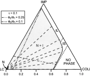
An example of phase diagram is plotted in Fig.2for ⌫ = 0.8,␭₂= 1,␹= 1,␶= 0.1,⌫R= 0.006, and␭3= 1.35. The last

two values have been chosen in order that there exists a two-phase coexistence region共gray region in the phase dia-gram兲 between a rich-in-colloid isotropic phase and a nem-atic phase in which the colloid concentration practically can-cels. This is typically what is observed experimentally with colloidal particles of diameter in the range of a few tens of nanometers. We recall that the colloids are expelled from the nematic phase because they distort the director field, which is unfavorable energetically. We shall note that points repre-senting the nematic phase are located in the lower part of the left side of the triangle 共corresponding to ⌽₃⬇0兲. We shall also emphasize that in the isotropic phase, the hard-sphere colloid is in the liquid state below the coexistence boundary ⌽3iso⬍0.52 and in the solid state at higher concentration

0.52⬍⌽3iso⬍⌽c= 0.637, where ⌽c is the random

close-packing fraction. Finally, for ⌽3iso⬎0.637, no phase is

de-fined by the model.

From this phase diagram, we can describe two comple-mentary situations which could be test experimentally. First, we can add impurities to a given mixture of liquid crystal and colloids of constant ratio ⌽3/⌽1, for instance ⌽3/⌽1

= 0.10. This is what happens in the experiments performed with PMMA colloids where the remnant alkane slowly dif-fuses in the mixture or is directly added.12,14,15The followed path in this case corresponds to the dashed–double dotted

FIG. 1. Phase diagram for nematic–non-nematic binary mixture for⌫=0.8, ␭2= 1, and␹= 1.

FIG. 2. Phase diagram calculated for a three-component system consisting of liquid crystal, impurities, and colloids. The solid curve refers to the bin-odal. Inside the gray region, there is phase separation. The dashed lines give the volume fractions of each species in the two phases at their intersections with the bimodal. Along the dashed-dotted line共the dotted line兲, ⌽2/⌽1

= 0.25共⌽3/⌽1= 0.10兲. In the isotropic phase, the hard-sphere colloid is in

the liquid state共IL兲 below the coexistence boundary ⌽3iso⬍0.52, whereas it

is in the isotropic solid state共IS兲 at higher concentration 0.52⬍⌽3iso⬍⌽c

line in the ternary phase diagram. Starting from the bottom of phase diagram, we immediately see that adding impurities to the mixture tends to simultaneously increase the impurity concentration and decrease the colloid concentration in the isotropic phase, whereas the liquid crystal remains almost pure in the nematic phase. As a result, the colloid, which initially forms a solid phase, melts to give a disordered sus-pension when the impurity concentration is sufficiently large 共in this example, when ⌽2⬎0.09兲.

Second, we can add colloids to a well-defined mixture of liquid crystal and impurities 共imposing, for instance, ⌽2/⌽1= 0.25兲. In this case, we follow the dashed-dotted line

in the ternary phase diagram. Starting from the left of the phase diagram, we immediately note that when⌽3increases,

the impurity concentration strongly decreases in the isotropic liquid, whereas the liquid crystal remains almost pure in the nematic phase as in the previous case. As for the colloidal particles, they first form a disordered suspension in the iso-tropic liquid to finally solidify when⌽₃exceeds 0.52.

In the next section, we show that changing the concen-trations of the different species along a given path leads to large variations of the nematic-isotropic surface tension.

IV. INTERFACIAL TENSION

We consider a planar nematic-isotropic interface of unit surface area in equilibrium and take the z axis perpendicular to the interface. We choose the origin z = 0 such that the nematic phase共S=Snem兲 lies in the region z⬍0 and the

iso-tropic phase共S=0兲 in the region z⬎0. The free energy func-tional共3兲 can be expressed as共by using real variables兲

F =

冕

−⬁ ⬁ dz

冋

f +1 2K⌽2共dz⌽2兲 2₊1 2K⌽3共dz⌽3兲 2 +1 2KS共dzS兲 2

册

_{. 共13兲}

The interfacial tension␥is defined as the difference, per unit area of the interface, between the actual free energy of the system and that of the two phases if each were uniform and isolated. It is thus given by

␥= f₀

冕

−⬁ ⬁ dz

冋

⌬g +1 2l⌽2 2 _共d z⌽2兲2+ 1 2l⌽3 2 _共d z⌽3兲2 +1 2lS 2_共d zS兲2

册

, 共14兲

where⌬g=g共S共z兲,⌽2共z兲,⌽3nem兲−g共0,⌽2iso,⌽3iso兲 is the

di-mensionless energy difference calculated from Eq.共11兲and S the order parameter normalized to its value in the pure liquid crystal 共S⬅S/Snem 0兲. The three correlation lengths are

de-fined to be lS=共KSSnem 02 / f0兲1/2, l⌽2=共K⌽2/ f0兲

1/2_{, and l} ⌽3

=共K_⌽

3/ f0兲

1/2_{. As we shall see later, they give the typical}

widths of the profiles in S,⌽2, and⌽3, respectively.

Minimizing the functional in Eq. 共14兲 with respect to ⌽2共z兲, ⌽3共z兲, and S共z兲, we obtain the corresponding

Euler-Lagrange equations for the equilibrium profiles of the order parameter and of the impurity and colloid compositions,

l_⌽ 2 2 _d z 2_⌽ 2= ⳵⌬g ⳵⌽2 , 共15兲 l_⌽ 3 3 _d z 2_⌽ 3= ⳵⌬g ⳵⌽3 , 共16兲 lS 2 dz 2 S =⳵⌬g ⳵S , 共17兲

with the following boundary conditions共i=2,3兲: 共⌽i,S兲 =

再

共⌽inem,Snem兲 as z → − ⬁

共⌽iiso,0兲 as z→ ⬁,

冎

共18兲 and dz⌽i共±⬁兲=dzS共±⬁兲=0.

Multiplying Eq.共15兲by dz⌽2, Eq.共16兲by dz⌽3, and Eq.

共17兲by dzS, adding the resulting equations, and then

integrat-ing once with respect to z, we obtain ⌬g =1 2l⌽₂ 2 _共d z⌽2兲2+ 1 2l⌽₃ 2 _共d z⌽3兲2+ 1 2lS 2_共d zS兲2. 共19兲

Using this expression to eliminate⌬g term from Eq.共14兲, the interfacial tension becomes

␥= f0

冕

−⬁ ⬁ 关l_⌽ 2 2 _共d z⌽2兲2+ l_⌽2₃共dz⌽3兲2+ lS2共dzS兲2兴dz. 共20兲

To calculate ␥ we need the values of KS and K⌽_i 共i

= 2 , 3兲. For the former, we use the experimental value of KS= 2.1⫻10−12N given for 5CB in Ref.25, from which we

calculate lS= 1.7⫻10−8m by taking the previous values of

Snem 0 and f0. The stiffness coefficient K⌽₂ is unknown

ex-perimentally for a 5CB-alkane mixture. For this reason, we propose to take K_⌽

2/ KS= 40, as in Ref. 27, which gives

ex-plicitly K_⌽ 2= 3.8⫻10 −10_{N and l} ⌽2= 2.6⫻10 −7 _{m. As for} K_⌽

3, it must be very small in comparison with KS and K⌽2

because of the “large” size of the particles, so we shall take K_⌽

3= 0. In the following, we set K⌽2⬅K⌽ 共l⌽2⬅l⌽兲.

With this particular choice, the length scales are well separated because l_⌽ⰇlS. A direct consequence is that the

differential equations关共15兲–共17兲兴 are decoupled since on the distance over which each variable changes significantly, the others may be considered as constant. In practice, that means that in the right-hand side of each equation, Eqs.共15兲–共17兲, the partial derivative can be replaced by a total derivative. As a result the typical distances over which S and⌽ change are given, respectively, by lS and l␾˜. More precisely, it can be

checked numerically that the real profiles are very close to hyperbolic tangent profiles of the forms

⌽2共z兲 =

1

2

冉

⌽2nem+⌽2iso+共⌽2iso−⌽2nem兲tanh z

冑

2l_⌽

冊

, 共21兲 S共z兲 =Snem 2

冉

1 − tanh z

冑

2lS

冊

.

From these profiles and Eq.共20兲, we can immediately calcu-late the interfacial tension,

␥/␥S= Snem2 +共⌽2iso−⌽2nem兲2

冉

l_⌽ lS

冊

, 共22兲

where ␥S is the surface tension of the pure liquid crystal:

␥S=共

冑

2 / 6兲f0lS 关knowing that in this limiting case, the S共z兲

profile given in Eq.共21兲is exact兴. Note that in Eq.共22兲, Snem

is calculated from Eq. 共12兲, while ⌽2iso and ⌽2nem are the

concentrations calculated from the ternary phase diagram. We emphasize that all these quantities depend on the colloid concentration ⌽3. As a consequence, the surface tension

must change in the presence of the colloids, which is not obvious at the first sight from Eq.共22兲.

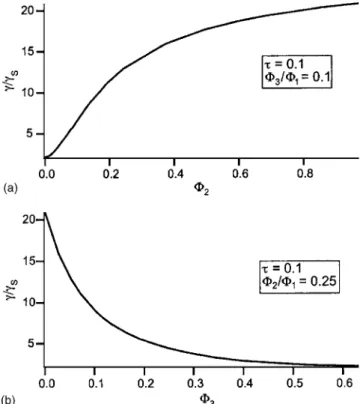
To illustrate this important point, let us return to the two experimental situations described at the end of the previous section. More precisely, let us discuss how the surface ten-sion changes when impurities 共colloids兲 are added to a colloid–liquid crystal mixture of a given composition⌽₃/⌽₁ 共to an impurity–liquid crystal mixture of a given composition ⌽2/⌽1兲. All calculations were performed at reduced

tem-perature␶= 0.1, by taking as reference surface tension ␥S of

value of 2.2⫻10−5_{N / m.}

In the first case 共corresponding to the dashed–double dotted line of equation⌽3/⌽1= 0.10 in Fig. 2兲, the reduced

surface tension ␥/␥S strongly increases when ⌽2 increases

关Fig.3共a兲兴. In the second case 共corresponding to the dashed-dotted line of equation⌽2/⌽1= 0.25 in Fig.2兲,␥/␥Sstrongly

decreases when ⌽3 increases关Fig.3共b兲兴. These large

varia-tions can be easily explained by considering that the term proportional to S_nem2 in Eq. 共22兲 is practically constant, whereas the second term, proportional to共⌽2iso−⌽2nem兲2

共al-ways very close to⌽_2iso2 as the nonmesogenic impurities are expelled from the nematic phase兲 strongly increases 共strongly decreases兲 when one adds impurities 共colloids兲 to the mixture. This can be seen immediately from the phase diagram by moving along the dashed–double dotted line共the dashed-dotted line兲.

We can expect that these large variations of the surface tension play an important role in experiments. Indeed, our calculations show that adding a small amount of impurity can strongly increase the nematic-isotropic surface tension 关Fig. 3共a兲兴. In contrast, adding colloids to an impure liquid crystal leads to an opposite effect 关Fig. 3共b兲兴. This second effect could explain qualitatively why the mesh size of the observed cellular superstructure decreases when the concen-tration of colloids is increased.14 The elastic modulus G

⬘

should also depend on the impurity concentration. Such ef-fects were indeed reported recently in experiments18but they are not yet well documented.

Another question that arises is how to measure the sur-face tension. This could be performed by using the sessile共or pendant兲 drop method,8,28provided that the colloid can flow in order that the drop equilibrates in the gravity field. Ac-cording to our calculations, this condition is fulfilled for small concentrations of colloids or large concentrations of impurities. In practice, it will also be necessary to break the cellular structure which spontaneously forms during the phase transition in order to separate the nematic phase from the isotropic one. This could be done by centrifugation, the colloid being generally more dense than the nematic phase, but one must be careful to not separate the colloids from the rest of the mixture, which is an experimental challenge. An alternative method to estimate the surface tension would be to look at the damping rate of the capillary waves at the flat nematic-isotropic interface, for instance, by using new devel-oped microscopy techniques which are more local than usual scattering techniques. This question, which represents in it-self another experimental challenge, is analyzed in detail in the next section from a theoretical point of view.

V. CAPILLARY WAVES A. Equations of motion

We assume that the heat diffusion is sufficiently rapid in order that the system remains at thermal equilibrium. We therefore ignore the equation for energy conservation and assume an isothermal system at a specified temperature. We further assume that the fluid is incompressible. Within these approximations, the equations of motion for the velocity and the nematic order parameter become29–31

⳵␣v␣= 0, 共23兲 ␳dv␣ dt =⳵␤共− p␦␣␤+␴␣␤ d +␴_␣␤v 兲 + ␦F ␦⌽2 ⳵␤⌽2␦␣␤, 共24兲 0 = h_␣␤+ h_␣␤v −␭␦_␣␤−⑀_␣␤␥␭_␥, 共25兲 where␳is the density and p the pressure, while␭ and ␭_␥are the Lagrange multipliers associated with conditions Tr Q = 0 and Q_␣␤= Q_␤␣, respectively. In this expression,␣,␤, and␥

FIG. 3.共a兲 Nematic-isotropic reduced interfacial tension␥/␥Sas a function

of impurity volume fraction⌽2for␶= 0.1 and⌽3/⌽1= 0.1.共b兲 The same

quantity as a function of colloid volume fraction⌽3for␶= 0.1 and⌽2/⌽1

= 0.25. ␥S is the nematic-isotropic interfacial tension for the pure liquid

run from 1 to 3, summation over repeated indices is implied,

⑀␣␤␥ is the Levi-Civita symbol, and d / dt is the total time

derivative⳵/⳵t + v ·ⵜ. The distortion stress␴d_{关which results}

from molecular displacement keeping the orientation fixed:

r→r+u共r兲 and Q_␣␤共r兲→Q_␣␤

⬘

共r

⬘

兲=Q_␣␤共r兲兴 and the elastic

molecular field h关which results directly from the virtual ori-entational distortion: Q_␣␤共r兲→Q_␣␤

⬘

共r兲兴 are obtained in the standard manner and read

␴␣␤d = − ⳵

F

⳵共⳵␣Q␥␳兲⳵␤Q␥␳, 共26兲

h_␣␤= −␦F/␦Q_␣␤. 共27兲

The viscous stress tensor␴v _{and the viscous molecular field}

hv _{are introduced through the consideration of entropy}

pro-duction in a dissipative flowing nematic. Within a tensorial description of the Ericksen-Leslie theory,31–33they are given by ␴␣␤v =␤1Q␣␤Q␮␯A␮␯+␤4A␣␤+␤5Q␣␮A␮␤+␤6Q␤␮A␮␣ +1₂␮2N␣␤−␮1Q␣␮N␮␤+␮1Q␤␮N␮␣, 共28兲 − h_␣␤v = −1₂␮2A␣␤+␮1N␣␤, 共29兲 where N_␣␤=dQ␣␤ dt + Q␣␮W␮␤− W␣␮Q␮␤ 共30兲

is the time rate of change of the order parameter with respect to the background fluid angular velocity, also known as the corotational time derivative. The quantities ␤1, ␤4, ␤5, ␤6,

␮1, and ␮2=␤6−␤5 are viscous coefficients which can be

expressed in terms of the Leslie coefficients 共␣i兲 and the

value of the order parameter S,31 while A_␣␤=1₂共⳵_␣v_␤+⳵_␤v_␣兲 and W_␣␤=1₂共⳵_␣v_␤−⳵_␤v_␣兲 are, respectively, the symmetric and antisymmetric parts of the velocity gradient tensor.

The impurity composition equation of motion takes the Cahn-Hilliard form34 d⌽₂ dt =⌫⌽ⵜ 2

冉

␦F ␦⌽2

冊

, 共31兲

where the transport coefficient⌫_⌽is assumed to be constant. The complete dynamics is described by Eqs. 共23兲–共25兲 and

共31兲.

We consider a two-dimensional flow with horizontal and vertical velocity components u and w in the x and z direc-tions, respectively, and we simplify the expressions共28兲and

共29兲by assuming that

␤1=␤5=␤6= 0, ␤4= 2␤, 共32兲

which give ␮2= 0.31 In terms of Leslie coefficients␣i, these

relations are equivalent to

␣1=␣5=␣6= 0, −␣2=␣3=␣= 9S2␮1/4,

共33兲

␣4=␤4= 2␤.

Within these approximations, the coefficient␤describes the dissipation due to shear flow 共shear viscosity兲, while ␮1 is

associated with the standard rotational viscosity ␥1=␣3−␣2

= 2␣= 9S2_␮ 1/ 2.

Using these hypotheses, the basic Eqs. 共23兲–共25兲 and

共31兲take the following forms:

0 =⳵xu +⳵zw, 共34兲 ␳du dt = −⳵xp +␩ⵜ 2_{u − K} Sⵜ2S⳵xS +

冉

⳵f ⳵⌽2 − K_⌽ⵜ2⌽2

冊

⳵x⌽2, 共35兲 ␳dw dt = −⳵zp +␩ⵜ 2_{w − K} Sⵜ2S⳵xS +

冉

⳵f ⳵⌽2 − K_⌽ⵜ2⌽₂

冊

⳵z⌽2, 共36兲 ␮1 dS dt = − ⳵f ⳵S+ KSⵜ 2_{S, 共37兲} d⌽2 dt =⌫⌽ⵜ 2

冉

⳵f ⳵⌽2 − K_⌽ⵜ2⌽2

冊

, 共38兲

where␩=␩iso=␤in the isotropic phase共when ⌽3= 0兲, while

␩=␩nem=共␣+ 2␤兲/2 in the nematic phase 关note that this

vis-cosity corresponds to the second Miesowicz visvis-cosity ␩b

共Ref.8兲 measured when the nematic phase is sheared parallel

to the director兴.

In what follows, we shall suppose that the stationary planar nematic-isotropic interface 共i.e., the base state of the system兲 is situated at z=0, such that the nematic lies in the region z⬍0 and the isotropic phase in the region z⬎0. The x axis is taken in the direction of the wave vector k of the perturbation along the interface. This is possible without loss of generality if the system is isotropic in x and y directions, which implicitly assumes that the director anchoring on the interface is homeotropic and the biaxiality of the nematic phase is negligible. In this way, the wave number k repre-sents the modulus of the two-dimensional wave vector in the plane of the interface. Due to thermal fluctuations, small am-plitude monochromatic waves of the form ⬀ exp共ikx−⍀t兲 develop at the interface. In our notation, k is the wave vector 共real number兲 and ⍀ is the angular frequency. The latter quantity is generally a complex number whose the real part gives the relaxation time 1 /R共⍀兲 of the wave and the imagi-nary part, the phase velocityI共⍀兲/k.

B. Dispersion relation

To obtain the dispersion relation we use the method of matched asymptotic expansions.35 The results obtained for similar systems using this method were extensively pre-sented previously.19,36–38 The method consists of matching the solution obtained in an outer region, where z is of the order of l_␩=␩2_{/␳␥⯝1⫻10}−2_{m, to that calculated in an}

in-ner region in which z is of the order of lS=共KSSnem 02 / f0兲1/2

⯝1.7⫻10−8 _{m. There are two outer regions共one, deep into}

the nematic phase, z→−⬁, and the other deep into the

tropic phase, z→ +⬁兲 in which the dominant physics is hy-drodynamics, i.e., the dissipation due to the shear flow. In contrast, the variations of the nonconserved order parameter S and of the conserved parameter⌽2 are the dominant

pro-cesses in the inner region.19

The corresponding dispersion relation is given by38

⍀共⍀ − ⍀S_⌽兲 = ⍀_␩2. 共39兲

The angular frequency ⍀S_⌽ 共corresponding to the inner

re-gion of size lS兲 fixes the angular frequency in the limit k

→⬁. It expresses in the form19 ⍀S⌽=

␥k2

␮1␥S/KS+共⌽2iso−⌽2nem兲2/2k⌫⌽

. 共40兲

The difference共⌽2iso−⌽2nem兲 is calculated for a colloid

com-position ⌽3 different from 0 accordingly with the ternary

phase diagram shown in Fig. 2.

As for⍀_␩, it gives the angular frequency in the opposite limit k→0 共corresponding to the outer region of dimension l_␩兲. It is identical to the classical capillary-wave dispersion relation for a sharp interface. It reads39,40

⍀_␩2

=

冋

1 + k共knem

2

+ k_iso2 兲 − 2k3 共knem+ kiso兲共k2− knemkiso兲

册

⍀0 2

, 共41兲

where⍀₀2= −␥k3_{/ 2␳ is the capillary-wave dispersion relation}

for ideal 共inviscid兲 fluids, k_nem= k共1−␳⍀_␩/␩_nemk2_兲1/2_{, and}

k_iso= k共1−␳⍀_␩/␩_isok2_兲1/2_{. The latter expression is exact if the}

viscosities of the two phases are constant. It turns out that in our case, ␩iso corresponds to the viscosity of a disordered

colloidal hard-sphere dispersion. As a consequence␩_isois not constant but depends on the angular frequency given here by R共⍀兲. According to de Kruif et al.,41

the viscosity of a dis-ordered suspension can be written as

␩iso=

␩0−␩⬁

1 + Pe +␩⬁, 共42兲

where ␩_⬁ and ␩₀ are the high- and low-frequency limiting viscosities, of expressions ␩⬁=␤

冉

1 −⌽3iso 0.63

冊

−2 , 共43兲 ␩0=␤

冉

1 − ⌽3iso 0.71

冊

−2 .

In Eq.共42兲, Pe is the Peclet number or the dimensionless angular frequency. This number measures the importance of hydrodynamic effects with respect to thermal ones. It is de-fined to be

Pe =6␲␤R

3_R共⍀兲

kBT

. 共44兲

In the following, we shall assume that Eq. 共41兲still applies on condition to use expression共42兲 for the viscosity of the isotropic liquid.

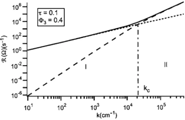
The real part of the solution of Eq. 共39兲 and its asymptotic limits given by Eqs. 共40兲and共41兲 are drawn in Fig.4for ␶= 0.1,⌽3= 0.4, and a radius of the colloidal

par-ticles R = 100 nm. To perform numerical calculations, we have taken the typical experimental values given in the lit-erature for 5CB:␣=␤= 0.01 Pa s and␳= 103_{kg/ m}3_.8

For the transport coefficient ⌫_⌽ introduced in Eq. 共31兲, we have taken ⌫_⌽= 4.5⫻10−13_m3_{s / kg. This value has been}

esti-mated by assuming that the typical molecular velocities vS

= lS/ tS and v⌽= l⌽/ t⌽ are equal. Note that here lS

=共KSSnem 02 / f0兲1/2, tS= 3␮1Snem2 / 2f0, l⌽=共K⌽/ f0兲1/2, and t⌽

= K_⌽/⌫_⌽f₀2.

Two regions can be clearly distinguished. In the short wavelength limit共region II兲, the interface is diffuse and the relaxation of the two order parameters is the dominant pro-cess. The dispersion relation is given by Eq. 共40兲 共dashed curve in Fig. 4兲. In the long wavelength limit, the viscous

damping process in the outer region dominates and the cor-responding dispersion relation is given by Eq. 共41兲 共dotted curve in Fig.4兲.

The transition between these two regions takes place whenR共⍀_␩兲=R共⍀S⌽兲. That gives the critical wave number

kc⯝2.1⫻104cm−1 corresponding to the critical wavelength

␭c⯝3⫻10−4 cm. In Fig.4, the influence of colloids on the

dispersion relation is not clearly visible. For this reason, we superposed in Fig. 5 the curves representing the dispersion relations of a ternary and a binary mixture. More precisely, in Fig. 5, the solid line refers to the previous ternary mixture with⌽₃= 0.4 and⌽₂/⌽₁= 0.25, whereas the dashed line has been calculated for a binary mixture with⌽2/⌽1= 0.25共and

⌽3= 0兲.

We observe that the presence of colloids tends to de-crease the damping rate mainly in the hydrodynamic regime. The effect increases when the wavelength increases. This can be explained by considering the influence of two factors. First, the colloids decrease the nematic-isotropic interfacial tension 共see Fig.2兲. In the case of the ternary mixture with

⌽3= 0.4, the interfacial tension has the value␥/␥S⬇4, while

for the binary mixture without colloids, ␥/␥S⬇21. This

ef-fect tends clearly to decrease the damping rate. Second, the colloids increase the viscosity of the isotropic phase 关see

FIG. 4. The damping rateR共⍀兲 as a function of k for the colloid compo-sition ⌽3= 0.4, reduced temperature ␶= 0.1, and the fixed ratio ⌽2/⌽1

= 0.25. The general dispersion relation关Eq. 共39兲兴 共continuous curve兲, the inner region dispersion relation关Eq. 共40兲兴 共dashed curve兲, and the outer region dispersion relation关Eq.共41兲兴 共dotted curve兲. It must be noted that in the whole range of wave vectors shown in this graph,⍀ is a real number so thatR共⍀兲=⍀ 共waves are overdamped兲.

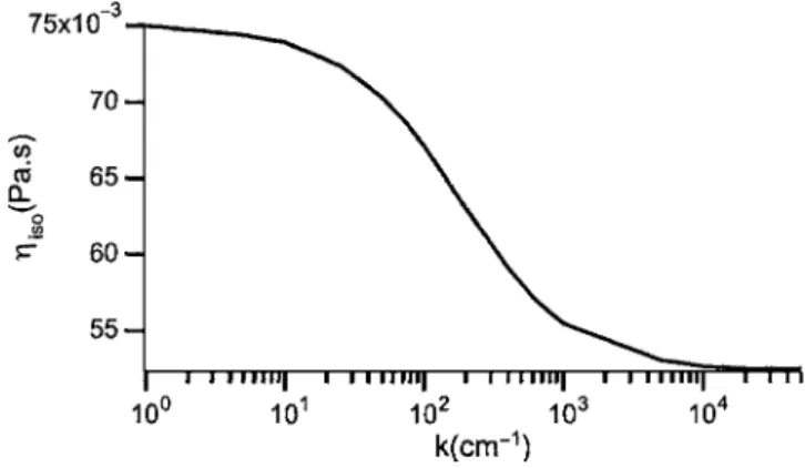
Eqs. 共42兲 and 共43兲兴. This effect also tends to decrease the damping rate. As can be seen from Fig.6where the viscosity of the isotropic phase 关given by Eq. 共42兲兴 is plotted as a function of the wave vector for ⌽₃= 0.4 and ⌽₂/⌽₁= 0.25, this effect is stronger below a typical wave vector of about 2⫻103cm−1. More precisely, this curve shows that the col-loids increase the viscosity by a factor of 7.5共with respect to the value without colloids兲 below this limit and by a factor of 5.3 above. The sum of these two effects explains the increase by one order of magnitude of the damping rate observed at large wavelength共Fig.5兲.

Coming back to Fig.5, we shall note in addition that the value of kc that defines the “transition” between

hydrody-namic and relaxation of the order parameter regimes differ in the two cases. Without colloids kc= kc2⬇4.3⫻104cm−1,

while kc= kc1⬇1.3⫻104cm−1 in the presence of colloids.

This result is expected inasmuch as the colloids tend to de-crease the damping rate mainly in the hydrodynamic regime. Finally, we shall note that our analysis only makes sense if the wavelength of the perturbation is larger than the mean distance between the colloidal particles. For colloidal par-ticles of radius R = 100 nm and a concentration⌽3= 0.4, this

condition is satisfied as long as k艋共3⌽3/ 4␲兲1/3共2␲/ R兲

⬇3⫻105_cm−1_{, which is the case in all our calculations.}

VI. CONCLUSIONS

In this paper we have examined a few properties of a three-component system composed of a liquid crystal, a non-nematogenic fluid共impurities兲, and colloids. This theoretical study was motivated by recent experimental observations showing that during the preparation of mixtures of a liquid crystal with PMMA spheres, a third component, alkane, slowly liberates from the particles and diffuses into the sus-pension. This phenomenon was shown to influence the mesh size of the cellular structure formed after the nematic-isotropic phase separation, as well as its rheological proper-ties.

In this context we have more explicitly studied the phase diagram and the static and dynamical properties of the nematic-isotropic interface. Our main results can be summa-rized as follows.

共1兲 If one adds colloids to a liquid crystal–impurity mixture of a given composition⌽2/⌽1, the colloids go into the

isotropic phase 共there are expelled from the nematic phase兲. In this case, we have shown that the impurity concentration decreases in the isotropic liquid so that the nematic-isotropic surface tension also decreases. 共2兲 Inversely, if one adds impurities to a liquid crystal–

colloid mixture of fixed composition⌽₁/⌽₃, they con-centrate into the rich-in-colloid isotropic liquid and the nematic-isotropic surface tension increases.

共3兲 Finally, capillary waves are strongly influenced by im-purities and colloids. This comes from the fact that their dispersion relation strongly depends both on the viscosity of the two phases and on the surface tension. In particular, we have shown that adding colloids to a liquid crystal–impurity mixture of a given composition ⌽2/⌽1tends to decrease the damping rate of the waves

because the surface tension decreases and the viscosity of the isotropic liquid increases.

We must nevertheless mention that our calculations are simplified as they neglect the coupling between the nematic director and the hydrodynamic flow, as well as the anchoring effect of the director at the interface. In addition, we did not use the complete set of Leslie viscosities and we assumed that the viscosity of the isotropic phase共without the colloids兲 is independent of the impurity concentration. In spite of these simplifications, we hope that our model retains the es-sential physics and will be helpful to better understand the microstructure and the rheological properties of the cellular networks formed in the coexistence region.

Finally, note that our calculations could be generalized in order to take into account the coupling between the interface oscillations, the director field, and the velocity. One could also include density effects, in particular, to study interfaces in lyotropic liquid crystals.

FIG. 5. The damping rateR共⍀兲 as a function of k for␶= 0.1 without col-loids 共dotted curve兲 and for a colloid concentration ⌽3= 0.4 共continuous

curve兲. In both cases, ⌽₂/⌽₁= 0.25. Without colloids, waves are over-damped above k⬇33.6 cm−1_{and start to propagate below. The arrow}

indi-cates the limit between these two regimes. In contrast, waves are over-damped in the case of⌽3= 0.4 in the whole range of wave vectors shown in

the figure共they would start to propagate below k⬇1.5 cm−1_兲.

FIG. 6. The viscosity of the isotropic phase as a function of k for␶= 0.1, for colloid concentration⌽3= 0.4, and the ratio⌽2/⌽1= 0.25.

ACKNOWLEDGMENTS

One of the authors 共V.P.-N.兲 thanks Ecole Normale Supérieure de Lyon for scientific hospitality and acknowl-edges support from CEEX-05-D11-76 共SIDISANIZ兲 Re-search Program.

1_{E. M. Terentjev, Phys. Rev. E 51, 1330共1995兲.}

2_{V. A. Raghunathan, P. Richetti, and D. Roux, Langmuir 12, 3789共1996兲.} 3_{O. V. Kuksenok, R. W. Ruhwandl, S. V. Shiyanovskii, and E. M.}

Ter-entjev, Phys. Rev. E 54, 5198共1996兲.

4_{R. W. Ruhwandl and E. M. Terentjev, Phys. Rev. E 55, 2958共1997兲; 56,}

5561共1997兲.

5_{T. C. Lubensky, D. Pettey, N. Currier, and H. Stark, Phys. Rev. E 57, 610}

共1998兲.

6_{H. Stark, Phys. Rep. 351, 387共2001兲.}

7_{P. G. de Gennes and J. Prost, The Physics of Liquid Crystals, 2nd ed.}

共Oxford University Press, New York, 1993兲.

8_{P. Oswald and P. Pieranski, Nematic and Cholesteric Liquid Crystals:}

Concepts and Physical Properties Illustrated by Experiments, Liquid

Crystals Book Series 共Taylor & Francis, London/CRC, Boca Raton, 2005兲.

9_{P. Poulin, V. A. Raghunathan, P. Richetti, and D. J. Roux, J. Phys. III 4,}

1557共1994兲.

10_{P. Poulin, H. Stark, T. C. Lubenski, and D. A. Weitz, Science 275, 1770}

共1997兲; P. Poulin and D. A. Weitz, Phys. Rev. E 57, 626 共1998兲.

11_{J.-C. Loudet, P. Barois, and P. Poulin, Nature共London兲 407, 611 共2000兲.} 12_{S. P. Meeker, W. C. K. Poon, J. Crain, and E. M. Terentjev, Phys. Rev. E}

61, R6083共2000兲.

13_{J. Yamamoto and H. Tanaka, Nature共London兲 409, 321 共2001兲.} 14_{V. J. Anderson, E. M. Terentjev, S. P. Meeker, J. Crain, and W. C. K.}

Poon, Eur. Phys. J. E 4, 11共2001兲.

15_{V. J. Anderson and E. M. Terentjev, Eur. Phys. J. E 4, 21共2001兲.} 16_{J. Cleaver and W. C. K. Poon, J. Phys.: Condens. Matter 16, S1901}

共2004兲.

17_{D. Vollmer, G. Hinze, W. C. K. Poon, J. Cleaver, and M. E. Cates, J.}

Phys.: Condens. Matter 16, L227共2004兲.

18_{D. Vollmer, G. Hinze, B. Ullrich, W. C. K. Poon, M. E. Cates, and A. B.}

Schofield, Langmuir 21, 4921共2005兲.

19_{V. Popa-Nita, T. J. Sluckin, and S. Kralj, Phys. Rev. E 71, 061706}

共2005兲.

20_{P. Ziherl, A. Šarlah, and S. Žumer, Phys. Rev. E 58, 602共1998兲; A.}

Šarlah and S. Žumer, ibid. 60, 1821共1999兲.

21_{P. van der Schoot, J. Phys. Chem. B 103, 8804共1999兲.}

22_{P. J. Flory, Principles of Polymer Chemistry共Cornell University Press,}

Ithaca, 1953兲.

23_{N. F. Carnahan and K. E. Starling, J. Chem. Phys. 51, 635共1969兲.} 24_{W. B. Russel, D. A. Saville, and W. R. Schowalter, Colloidal Dispersions}

共Cambridge University Press, Cambridge, 1989兲.

25_{S. Faetti and V. Palleschi, J. Chem. Phys. 81, 6254共1984兲; Phys. Rev. A}

30, 3241共1984兲; J. Phys. 共France兲 Lett. 45, L313 共1984兲.

26_{K. Denolf, B. Van Roie, C. Glorieux, and J. Thoen, Phys. Rev. Lett. 97,}

107801共2006兲.

27_{A. Matsuyama, R. M. L. Evans, and M. E. Cates, Eur. Phys. J. E 9, 79}

共2002兲; Z. Lin, H. Zhang, and Y. Yang, Phys. Rev. E 58, 5867 共1998兲.

28_{R. Williams, Mol. Cryst. Liq. Cryst. 35, 349共1976兲.} 29_{S. Hess, Z. Naturforsch. A 31A, 1507共1976兲.}

30_{P. D. Olmsted and P. Goldbart, Phys. Rev. A 41, 4578共1990兲; 46, 4966}

共1992兲; P. D. Olmsted and C.-Y. D. Lu, Phys. Rev. E 60, 4397 共1999兲.

31_{T. Qian and P. Sheng, Phys. Rev. E 58, 7475共1998兲.} 32_{J. L. Ericksen, Arch. Ration. Mech. Anal. 4, 231共1960兲.}

33_{F. M. Leslie, Q. J. Mech. Appl. Math. 19, 357 共1966兲; Arch. Ration.}

Mech. Anal. 28, 265共1968兲.

34_{J. W. Cahn, Trans. Metall. Soc. AIME 242, 166共1968兲.}

35_{M. H. Holmes, Introduction to Perturbation Methods共Springer-Verlag,}

New York, 1995兲.

36_{V. Popa-Nita and T. J. Sluckin, Phys. Rev. E 66, 041703共2002兲.} 37_{V. Popa-Nita and P. Oswald, Phys. Rev. E 68, 061707共2003兲.} 38_{V. Popa-Nita, P. Oswald, and T. J. Sluckin, Mol. Cryst. Liq. Cryst. 435,}

215共2005兲.

39_{L. D. Landau and E. M. Lifshitz, Fluid Mechanics共Pergamon, Oxford,}

1959兲.

40_{V. G. Levich, Physicochemical Hydrodynamics 共Prentice-Hall,}

Engle-wood Cliffs, NJ, 1962兲.

41_{C. G. de Kruif, E. M. F. van Iersel, and A. Vrij, J. Chem. Phys. 83, 4717}