Networks beyond pairwise interactions: structure and dynamics

HAL Id: hal-03094211

https://hal.archives-ouvertes.fr/hal-03094211

Submitted on 4 Jan 2021

HAL is a multi-disciplinary open access

archive for the deposit and dissemination of

sci-entific research documents, whether they are

pub-lished or not. The documents may come from

teaching and research institutions in France or

abroad, or from public or private research centers.

L’archive ouverte pluridisciplinaire HAL, est

destinée au dépôt et à la diffusion de documents

scientifiques de niveau recherche, publiés ou non,

émanant des établissements d’enseignement et de

recherche français ou étrangers, des laboratoires

publics ou privés.

dynamics

Federico Battiston, Giulia Cencetti, Iacopo Iacopini, Vito Latora, Maxime

Lucas, Alice Patania, Jean-Gabriel Young, Giovanni Petri

To cite this version:

Federico Battiston, Giulia Cencetti, Iacopo Iacopini, Vito Latora, Maxime Lucas, et al.. Networks

beyond pairwise interactions: structure and dynamics. Physics Reports, Elsevier, 2020, 874, pp.1-92.

�10.1016/j.physrep.2020.05.004�. �hal-03094211�

Federico Battiston∗

Department of Network and Data Science, Central European University, Budapest 1051, Hungary

Giulia Cencetti

Mobs Lab, Fondazione Bruno Kessler, Via Sommarive 18, 38123, Povo, TN, Italy

Iacopo Iacopini

School of Mathematical Sciences, Queen Mary University of London, London E1 4NS, United Kingdom and Centre for Advanced Spatial Analysis, University College London, London, W1T 4TJ, United Kingdom

Vito Latora†

School of Mathematical Sciences, Queen Mary University of London, London E1 4NS, United Kingdom Dipartimento di Fisica ed Astronomia, Universit`a di Catania and INFN, I-95123 Catania, Italy

The Alan Turing Institute, The British Library, London NW1 2DB, United Kingdom and Complexity Science Hub Vienna (CSHV), Vienna, Austria

Maxime Lucas

Aix Marseille Univ, CNRS, CPT, Turing Center for Living Systems, Marseille, France Aix Marseille Univ, CNRS, IBDM, Turing Center for Living Systems, Marseille, France and

Aix Marseille Univ, CNRS, Centrale Marseille, I2M, Turing Center for Living Systems, Marseille, France

Alice Patania

Network Science Institute, Indiana University, Bloomington, IN, USA

Jean-Gabriel Young

Center for the Study of Complex Systems, University of Michigan, Ann Arbor, MI, USA, 48109

Giovanni Petri‡

ISI Foundation, via Chisola 5, 10126 Turin, Italy and

ISI Global Science Foundation, 33 W 42nd St, 10036 New York NY, USA (Dated: June 3, 2020)

The complexity of many biological, social and technological systems stems from the richness of the interactions among their units. Over the past decades, a great variety of complex systems has been successfully described as networks whose interacting pairs of nodes are connected by links. Yet, in face-to-face human communication, chemical reactions and ecological systems, interactions can occur in groups of three or more nodes and cannot be simply described just in terms of simple dyads. Until recently, little attention has been devoted to the higher-order architecture of real complex systems. However, a mounting body of evidence is showing that taking the higher-order structure of these systems into account can greatly enhance our modeling capacities and help us to understand and predict their emerging dynamical behaviors. Here, we present a complete overview of the emerging field of networks beyond pairwise interactions. We first discuss the methods to represent higher-order interactions and give a unified presentation of the different frameworks used to describe higher-order systems, highlighting the links between the existing concepts and representations. We review both the measures designed to characterize the structure of these systems, and the models proposed in the literature to generate synthetic structures, such as random and growing simplicial complexes, bipartite graphs and hypergraphs. We then introduce and discuss the rapidly growing research on higher-order dynamical systems and on dynamical topology. We focus on novel emergent phenomena characterizing landmark dynamical processes, such as diffusion, spreading, synchronization and games, when extended beyond pairwise interactions. We elucidate the relations between higher-order topology and dynamical properties, and conclude with a summary of empirical applications, providing an outlook on current modeling and conceptual frontiers.

∗ _{[email protected]} †_{[email protected]} ‡_{[email protected]}

CONTENTS

I. Introduction 3

II. Higher-order representations of networks 5

A. Elementary representations of higher-order interactions 5

1. Low- versus high-order representations 5

2. Graph-based representations 5

3. Explicit higher-order representations 7

B. Relations and links between representations 8

III. Measures 9

A. Matrix representations of higher-order systems 10

1. Incidence matrix 10

2. Adjacency matrix 10

B. Walks, paths and centrality measures 11

1. Degree centralities 11

2. Paths and path-based centralities 13

3. Eigenvector centralities 14

C. Triadic closure and clustering coefficient 15

D. Simplicial homology 16

1. Boundary operators and homology groups 16

2. Evolving simplicial complexes 16

3. Other measures of shape in simplicial complexes 17

E. Higher-order Laplacian operators 17

1. Hypergraph Laplacians 18 2. Combinatorial Laplacians 18 IV. Models 20 A. Equilibrium models 21 1. Bipartite models 21 2. Motifs models 24

3. Stochastic set models 25

4. Hypergraphs models 27

5. Simplicial complexes models 29

B. Out-of-equilibrium models 31

1. Bipartite models 32

2. Stochastic set models 33

3. Hypergraphs models 33

4. Simplicial complexes models 34

V. Diffusion 36

A. Higher-order diffusion 37

1. Edge-flows 38

B. Higher-order random walks 39

1. Random walks on simplicial complexes 39

2. Random walks on hypergraphs 40

VI. Synchronization 43

A. Phase oscillators 43

1. Higher-order Kuramoto model 43

2. Higher-order interactions from phase reduction 50

B. Nonlinear oscillators 52

1. Chaotic oscillators 52

2. Neuron models 53

C. Inference of nonpairwise interactions in coupled oscillators 55

VII. Spreading and social dynamics 57

1. Spreading on simplicial complexes 58

2. Spreading on hypergraphs 59

B. Opinion and cultural dynamics beyond pairwise interactions 61

1. Voter model 61

2. Majority models 63

3. Continuous models of opinion dynamics 64

4. Cultural dynamics 65

VIII. Evolutionary games 65

A. Multiplayer games on networks 67

1. Public goods game 67

2. Other multiplayer games 69

B. Games with higher-order interactions 69

1. Public goods game on bipartite networks 69

2. Public goods game on hypergraphs 70

IX. Applications 71

A. Social systems 72

B. Neuroscience and brain networks 75

C. Ecology 78

D. Other biological systems 83

X. Outlook and conclusions 85

Acknowledgments 87

References 88

I. INTRODUCTION

Any significant understanding of a complex system must rely on system level descriptions. Consider the following exercise: take an ecosystem, and break it into its pieces. No matter how good or accurate our knowledge at the level of the individual species is, chances are that our understanding of population dynamics (e.g. how the abundances of the different species change in time) will be slim at best. The same holds true when we attempt to explain epileptic seizures starting from the individual neurons of the human brain; or viral rumors spreading across societies from individual human psychology. All these approaches fail because they are missing a fundamental ingredient of any complex system, that is the rich pattern of nonlinear interactions between the system components. After many years of reductionism, science has abandoned the idea that the collective behaviors of a complex system can be simply understood and predicted by considering the units of the system in isolation [1], and now more than ever is embracing the idea of complexity as one of the principles governing the world we live in.

Within this paradigm, networks have emerged as a reference modeling tool for complex systems [2]. Networks are the maps that define the physical or virtual space where interactions take place. Add competitive and cooperative relationships to an ecosystem, synaptic connections to the human brain, and human interactions to rumor spreading, and readily the self-organizing patterns and the collective behavior we observe in nature begin to unravel and look less obscure. Building on earlier work in mathematics, social network analysis and ecology, a handful of breakthrough papers at the turn of the millennium has attracted the interest of the scientific community, triggering thousands of contributions over the last twenty years and leading to the formation of the new multidisciplinary field of Network Science. This new research community has developed an unusual mixture of graph theory and statistical mechanics into a flourishing discipline, with applications spanning the full range of science, from fundamental physics all the way to the social sciences. The boundaries and potential applications are yet to be fully realized [2]. Still, the richness in scope and tools has already made the field of networks an independent discipline, often referred to as a science of its own. The growth of network science was also strengthened by the progressively wider availability of large datasets with detailed information on social, technological and biological interactions, which provided the raw material for the empirical validation of network models and predictions. We refer the reader interested in a first approach to network science to the several early review papers [3–6] and textbooks [7–10] on the subject.

As exploration of real-world systems deepens, network scientists are realizing the need to further characterize and enrich the relationships captured by a network description. This, however, creates problem: networks have originally

been understood as a collection of nodes, representing the elementary units of the system, and edges, describing the existence of interactions between pairs of such units. Applications to real-world systems, however, require the possibility to describe more details of an interaction [11], like for example: directed edges to describe the origin and destination of a message; edge weights, to highlight the intensity of an interaction; and even signs on the edges to distinguish whether a link encodes a productive or detrimental interaction among two units. In more recent years, a large effort has been devoted to formalize and develop the mathematical tools to analyze temporal networks, where interactions are not static but unfold in the temporal dimension [12]. Similarly, many works have recently considered the case of interacting systems where units can be connected by links of different nature, and which can be effectively represented in terms of multiplex networks or multilayer networks [13].

All these aspects have contributed in many cases to a better network representation, but are networks themselves enough to provide a complete description of a complex system?

The fundamental limit of networks is that they capture pairwise interactions only, while many systems display group interactions. Indeed, in social systems, ecology and biology among other examples, many connections and relationships do not take place between pairs of nodes, but rather are collective actions at the level of groups of nodes. For instance, three or more species routinely compete for food and territory in complex ecosystems [14]. In other cases, the presence of a third species influences the interaction between other two, affecting directly the interaction (the link) rather than the species involved (the nodes). Similarly, social mechanisms, such as peer-pressure, inherently go beyond the idea of dyadic connections. Collective interactions are not an entirely new idea, and to some degree have appeared in early research on networks. Think for instance to the majority-rule model for the dynamics of opinion formation, or the public goods game in evolutionary game theory. In addition to these examples, one of the most successful streams of research in network science in recent years, complex contagion, naturally accounts for multiple simultaneous interactions [15]. However, in all cases these applications tried to leverage the language of pairwise networks to describe interactions of higher order, for example by using bipartite graphs [16]. Can we instead find mathematical frameworks that can explicitly and naturally describes group interactions?

Simplicial complexes and hypergraphs are the natural candidates to provide such descriptions. And indeed, over the last few years, a wave of enthusiasm for these representations has revolutionized our vision of and ability to tackle real-world systems characterized by more than simple dyadic connections. The importance of high-order interactions had been recognized already a long time ago [17–19], but this rejuvenated interest has brought a new, and much deeper understanding of higher-order representations. There are no doubts now that moving beyond dyadic interactions is fundamental to explain and predict collective behaviors that could not be described before.

The aim of this report is to provide a review of the state-of-the-art on the structure and dynamics of complex networks beyond pairwise interactions, as well as a reference and perspective on crucial open questions in the field. Together with this introduction, the report is organized as follows:

• The first part (SectionsIItoIV) focuses on the structure of systems with higher-order interactions. In particular, Section II provides an introduction to the mathematical frameworks underlying higher-order representations. Section III describes the most common measures and properties currently used to describe the structure of systems with many-body interactions. Finally, Section IVreviews random models of higher-order systems and how they are used to make statistical inferences.

• The second part (Sections V to VIII) focuses on the dynamics of systems with higher-order interactions. In more detail, Section V discusses models of higher-order diffusion. Section VI describes the generalization of oscillator models and synchronization. SectionVIIintroduces recent models of spreading in social systems with group structure. SectionVIIIreports on models of competition and cooperation among multiple agents. • Finally, SectionIXis an overview of real-world applications to systems with higher-order interactions. Our final

conclusions and outlook are presented in SectionX.

We conclude this preamble with a final remark. The idea to include higher-order interactions in network analysis is very simple. To this end, going beyond pairwise interactions might not look harder than attaching weights or signs to the edges of a graph. Yet, in practice, moving from pairs to a more complicated interaction structure is a difficult issue, and it requires a great deal of sophistication and novel mathematical tools. This explains why the analysis of this aspect of complex system has been heavily delayed compared to its weighted and signed, and even temporal and multilayer counterparts. After all, classical physics already knew this: while a closed-form solution is available for the two-body problem, solving for the trajectories of n interacting bodies given their positions and momenta is still an open problem!

II. HIGHER-ORDER REPRESENTATIONS OF NETWORKS

A. Elementary representations of higher-order interactions

1. Low- versus high-order representations

We begin by first defining more precisely what we consider as interactions and, as a consequence, as higher-order interactions. We define an interaction as a set I = [p0, p1, . . . , pk−1] containing an arbitrary number k of basic elements of the system under study, which we indicate as nodes or vertices. Such interactions can then describe different situations in real systems, e.g. the coauthors of a scientific paper, a set of genes required to perform a certain function, the coactivation of a group neurons during a specific task, etc. In a slightly counterintuive way, we will denote the order (or dimension) of an interaction involving k nodes to be k − 1: a node interacting with itself only is a 0-order interaction, an interaction between two nodes has order 1, one among three nodes has order 2, and so on. Furthermore, we consider higher-order interactions to be k-interactions with k ≥ 2. Conversely, low order interactions are those characterized by k ≤ 1. In plain terms, low order systems are those in which only self-or pair-wise interactions take place (like edges in a graph), while higher-self-order systems (HOrSs, from now on) display interactions in groups of more than two elements.

The distinction between low- and high-order interactions is needed for two reasons. First, it highlights the differ-ences between the graph-theoretic descriptions, that shaped the study of complex systems in recent decades, and the more recently (re)proposed descriptions based on genuine group interactions. Secondly, it allows us to clearly frame the connections between such descriptions, their various overlaps and reciprocal mappings. Finally, our definition explicitly leaves out other types of higher-order dependencies between the components of a system, as for example those defined by multiple link types in multilayer networks [13,20–23], or by non-Markovian paths in time-stamped interaction data [12,24]. While these are out of the scope of this review, the interested reader can find an extensive discussion of these topics in the references mentioned above.

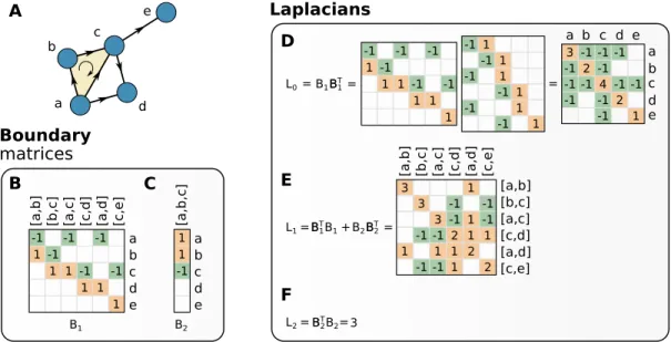
We define an interacting system (V, I) as the family of interactions I = {I0, . . . In} taking place on a node set V . To aid the intuition, let us make a specific example. Consider the node set V = [a, b, c, d, e] and the set of interactions I = {[a, b, c], [a, d], [d, c], [c, e]} (Fig.1A). I contains three 1-interactions and one 2-interaction. While the complete information about the systems is included in the list above, the study of most interesting properties of the system requires the choice of a representation. For example, measuring the collective effects of the interactions on a specific node requires the capacity to map interactions of different orders in a way that makes them comparable to each other; asking how dense the system is, or whether one node is reachable from another, again requires being able to compare in a controlled way interactions of different order and composition.

2. Graph-based representations

Graphs are the most common way to represent families of interactions (Fig.1C). A graph G = (V, E) is defined by a nodeset V with n elements, and an edgeset E whose m elements are pairs of nodes. A graph is then a collection of edges connecting pairs of nodes. In other words, the building blocks of graph representations are 1-interactions, i.e. interactions of the type I = [i, j]. The most natural choice is then to unfold each higher-order interaction in I in terms of 1-interactions built from pairs of nodes in I. Under this assumption, our example I = {[a, b, c], [a, d], [d, c], [c, e]} maps to IG= {[a, b], [b, c], [c, a], [a, d], [d, c], [c, e]} (Fig. 1B). This mapping makes systems amenable to be studied using tools developed in both graph theory [25] and network science [7]. Indeed, graph representations enabled the growth, depth and breadth of results on real-world complex networks in the last two decades [8–10], with applications spanning biology [26, 27], ecology [28, 29], social science [30, 31], engineering [32, 33], neuroscience [34–36], all the way to cosmology [37].

Despite the power of graph representations to capture many properties of complex interacting systems, their limits are easily identified: it is impossible to explicitly describe group interactions, or in other terms there is no direct relationship between I and IGnor any way to recover the former from the latter. For example, going back to our toy example, at the description level provided by IG, it is impossible to tell (and hence to describe) whether the original interaction set contained [a, c, d] or not. Naturally, in some cases networks can provide information on higher-order interactions, but these are always inferences based on the low order interactions, obtained for example by looking for very dense subsets of nodes using community [38], clique [39] or block detection [40] techniques. However, such

DATA about interactions: [a,b,c],[a,d],[d,c],[c,e]

link

Building blocks: GRAPH

a

b c

e

d

a b c d e

The top layer BIPARTITE GRAPH

>

describes groups NETWORK MOTIFS

>

Special type of motifs CLIQUES > a b c e d [a,b,c] [a,d] [c,d] [c,e] [c,d] [c,e] [a,d]

Simplices allow to differentiate

They require all subfaces:

Relaxing this condition

VS [a,b,c] [a,b] [b,c] [a,c] SIMPLICIAL COMPLEX HYPERGRAPH a b c e d [a,b,c] [a,b] [b,c] [a,c] [a] [b] [c] > > [a,b,c] Building blocks:

1-simplex 2-simplex 3-simplex 1-hyperlink 2-hyperlink 3-hyperlink

PAIRWISE REPRESENTATION

HIGHER ORDER REPRESENTATION A B G D E F C H L I J K

FIG. 1. Representations of higher-order interactions. A set of interactions of heterogeneous order (A) can be represented using only pairwise interactions (B). Using only low order blocks, the set of interactions can be described in th simplest way by using a graph (C). Alternatively, interactions can be encoded as nodes in one layer of a bipartite graph, where the other layer contains the interaction vertices (D). Other examples of high-order coordinated patterns can be encoded using motifs, small subgraphs with specific connectivity structures (E). Among motifs, cliques are especially popular as they represent the densest subgraphs, aking to higher order bricks (F). All these representations discard information that was present in the original interaction data (A). A solution is to consider explicitly higher order building blocks, in the form of simplices and hyperedges (G). Collection of simplices form simplicial complexes (H), which allow to discriminate between genuine higher order interactions and -even complex- sums of low order ones (I). Unfortunately, simplicial complexes, given a simplex, require the presence of all possible subsimplices (J), which can be too strong an assumption in some systems. Relaxing this condition effectively implies moving from simplices to hyperedges (K), which are the most general—and less constrained—representation of higher-order interactions (L).

reconstructions are often incomplete and rife with problems [41–43].

Bipartite graph representations effectively describe group interactions. Solidly within the realms of low-order interactions, bipartite graphs are graphs defined by two nodesets (U, W ) and edgeset E containing only edges (u, w) such that u ∈ U and w ∈ W . To represent higher-order interactions, one chooses U to coincide with the original nodeset V , i.e. U = V , and W to coincide with the set of interactions I [44, 45]. The links in the bipartite graph connect a node (in V ) to the interactions (of arbitrary order) in which it takes part (Fig. 1D). This representation emerges naturally in many fields: it is used for example in social sciences, where it provides a way to encode the membership of individuals to groups of different dimensions [46,47]; or to describe the collaboration of actors (nodes) in movies (interactions) [48]; it is also used in ecological bipartite graphs, where species linked to a common prey represent competition for resources among more than two species [29]; in recommendation systems [49] they describe the relations between customers and purchased products, and so on.

It is easy to see that the entire information in our toy model is preserved when interactions are described as a bipartite graph. In fact, this representation is very general and can indeed well mimic most interaction structures. However, at difference with other multilayer graph formulations [13,20], in a bipartite graph the nodes of the original system do not interact directly with each other anymore. Rather, their relation is always mediated by the interaction layer, which is of a different nature from the node layer itself. This implies that any measure or dynamic process define on the bipartite representation needs to take into account this additional complexity. The usual workaround to this problem is to consider the unipartite networks obtained by projecting the bipartite on one of the two layers.

Each interaction becomes then a fully connected subgraph among the nodes belonging to the interaction, losing the group structure in the same way as in the simple graph case. In addition, it is usually impossible to translate the information contained in the standard graph operators (e.g. Laplacian) defined on a bipartite graph into the ones corresponding to the unipartite projections [50,51]

Motifs allows to extract additional information on the properties of an interaction. They are the—usually small— recurrent subgraphs of a given network, or of a class of networks of similar origin [52]. Motifs are defined as specific patterns of edges (1-interactions) between vertices that appear to be statistically significant in the network (Fig.1E). They are considered structural signatures of the function of a network. That is, different motifs can correspond and reflect different functions or different optimization solutions to the same function [53]. Typically, the statistically validated frequencies (z-scores) with which the various motifs are observed in a network are collected into a motif profile, which can then be used for example to discriminate between different networks [54], e.g. between brain functional networks in different states [55, 56] or between differently evolved biological networks [27, 53, 57]. Motifs also found widespread application in the study of social [58] and temporal [59,60] systems.

Motifs constitute a refinement of the bipartite representation of a system, since, in addition to a division in groups akin to that of bipartite graphs, they allow to specify the interaction pattern in which a node is involved. The drawback to this is that the number of possible motifs to investigate grows exponentially with the number of nodes involved. This unfortunately makes them quite unwieldy as a descriptive tool for large graphs and/or motifs. As an example, generative models aimed to quantify randomness in networks via motif-based constraints [61] were shown to become very hard to manage, or even sample, for interactions above order 2 [62].

Because of the exponential growth in the number of motifs, a large part of the work on analyzing subgraphs focuses on a special type of motifs: cliques (Fig.1F). A clique of size k is defined as a fully connected subgraph of k nodes. Here, we use size for cliques to avoid confusion, since a k-clique usually encodes an interaction of order k − 1. The interest in cliques is justified also by the fact that they represent the most obvious definition of group from a network point of view, because they are the densest and most uniform motif [63]. Also, they directly encode the idea that every member of the clique interacts with every other [64,65]. Due to these properties, cliques are privileged building blocks of a network and its communities [39]. However, we can incur into problems if we want to use cliques to characterize higher-order interactions. In fact, going back to our toy example, we see that both sets a, b, c and a, d, c form 3-cliques. Conversely, in IG we only had a true 2-interaction, namely [a, b, c], while the fictitious interaction [a, d, c] is emerging as a byproduct of the union of the 1-interactions [a, d] and [d, c] with the [a, c] edge induced by [a, b, c]. We can see then that, by considering all cliques present at the graph level, we would “fill” a 2-interaction that was not included in the original interaction set. This is somewhat opposite to what happened when we considered the edges alone. In that case, we lost completely the notion of group. In the case of cliques instead, we risk “filling” too much and thus creating high-order interactions that were not there to begin with.

3. Explicit higher-order representations

To properly describe higher-order interactions, we need to encode them explicitly. Why not encoding interactions exactly as they are in fact? Simplices are the simplest mathematical objects to accomplishes this. The formal definition of simplices mimicks very closely the one we gave of higher-order interactions. In fact, a k-simplex σ is, in its most general form, just a set of k + 1 nodes σ = [p0, p1, . . . , pk] (Fig. 1G). This notation is the standard one borrowed from the literature in algebraic topology [66], where nodes are often points in a topological space. In applications where the interactions are purely combinatorial, one might want to draw attention to the interactions rather than to the underlying space. Thus, in these cases, nodes are often denominated as v0, v1, . . . to highlight that they are vertices of interactions, without any reference to an underlying space. The definition of dimension of a simplex coincides then with the definition of order of an interaction we gave earlier. Based on this parallel between the definitions of interactions and simplices, it is easy to see that we do not incur anymore in the problems described above. However, it is not clear how we can handle interactions of potentially different dimensions together and which are the advantages of such representations. Just like graphs are collections of edges, simplicial complexes are collections of simplices (Fig. 1H). At difference with graphs, they require further properties to be considered valid complexes: a collection of n simplices K = {σ0, σ1. . . σn} is a valid simplicial complex if, for every k-simplex σ = [p0, p1, . . . , pk] ∈K, all its subfaces of any dimensions belong to K too. For example, if the triangle [a, b, c] ∈ K, then we also require [a], [b], [c], [a, b], [a, c], [b, c] to belong to K. Note that if we were to extract cliques from a graph and consider them as simplices (which is the operative definition of a clique complex ), it would be impossible to distinguish the two cases in which respectively the triangle was present or not. Using a simplicial formalism instead

this distinction is immediate, as we only need to check whether the 2-interaction [a, b, c] is included in K (Fig.1I). Simplicial descriptions are very powerful because they come equipped with many nice mathematical gadgets. It is in fact straight-forward to define Laplacian operators for any dimension on simplicial complexes [67, 68], they can approximate both regular manifolds and highly irregular structures [69, 70], and they come naturally equipped with boundary operators stringing together simplices with different dimensions. Crucially, these operators describe the topology and shape of simplicial complexes in terms of their cycles, cavities and higher-order topological holes [71] and are naturally related to the combinatorial Laplacians [68]. In the following sections, we will describe many of these properties in greater detail, because they represent some the most powerful tools currently available and are the foundation of recent advances in topological data analysis [72–74].

Although simplicial complexes overcome some of the problems encountered by other lower dimensional representations, they are still quite limited by the requirement on the existence of all subfaces. In some cases, this constraint is too restrictive. For instance, when studying social systems, it is important to be able to describe interactions in groups. In this case we can use simplicial complexes as it is rather safe to assume that a group interaction also implies the underlying pairwise interactions (Fig.1J). The relative importance of pairwise versus group interactions can then be encoded in weights over the simplices.

However, in other cases, the inclusion constraint can be less easily justified: suppose for example that we are studying collaborations in scientific papers, and we observe a paper by three authors and none by the corresponding pairs of authors; or gene pathways were exactly three genes are needed to perform a function, but the subgroups are not responsible for any function on their own. Clearly, it would be useful to be able to describe also these situations (Fig.1K).

Hypergraphs provide the most general and unconstrained description of higher-order interactions. Formally, a hypergraph is defined by a nodeset V and a set of hyper-edges H that specify which nodes participate in which way within an interaction. Each hyper-edge is a non-empty subset of V . It is easy to see that hypergraphs are the most appropriate description of interacting systems (V, I) that we gave at the beginning of the section (Fig. 1L). Notice that a hypergraph can include the 2-interaction [a, b, c] without any requirement on the existence of 1-interactions [a, b], [a, c] and [b, c]. In fact, hypergraphs are so unconstrained that it is also possible to define hyperedges that include other hyperedges, e.g. given v, w, z ∈ V and γ = [v, w] ∈ H, it is possible to define a new hyperedge γ′_{= [z, w, v; γ] ∈ H.} Such extreme flexibility comes, as expected, with an additional complexity in treating them. For example, while many graph-theoretic concepts can be extended to the case of hypergraphs, such an endevour is often fraught with complications [75], to the point that a proper definition of Laplacian operators [76] on hypergraphs and of their properties, e.g. the spectral diameter, has only emerged in the few last years [77, 78] and—to the best of our knowledge—has found few real world applications, e.g. degree-generating models [79] and hypergraph modularity [80,81].

B. Relations and links between representations

Naturally, many questions emerge when discussing different representations of the same interacting system: how much overlap is there among two different representations? Is it possible to map one onto another in a canonical way? What kind of information is preserved (and lost) when moving between representations? For example, it seems obvious that a simplicial complex composed only by 1-dimensional simplices (edges) should be the same thing as a graph, right?

Well, it depends. Let us illustrate the links between representations starting from simplicial complexes (Fig. 2A). There are many ways of writing down a simplicial complex, but we focus here only on two descriptions, that are equally valid yet carry very different meanings: the Hasse diagram and the facet representation.

The Hasse diagram of a simplicial complex K is the directed acyclic graph HD(K) = (VHD, EHD), whose nodeset VHD contains a node for each simplex in K (VHD = {σ}∀σ ∈ K), while the edgeset EHD contains an edge for each inclusion between simplices that differ in dimension by 1 . In other terms, for two simplices σ, τ ∈ K there exist an edge (σ, τ ) ∈ EHD iff σ ⊂ τ and dim(τ ) = dim(σ) + 1. In Fig. 2B we provide an example of a Hasse Diagram for a toy simplicial complex (Fig.2A) . It is easy to see that the Hasse Diagram unfolds all the structure in the simplicial complex, by making explicit the hierarchy of simplices in the complex via its multipartite structure (one layer per dimension), and thus providing information about its internal organization. Importantly, it also gives an explicit way to walk on a simplicial complex: starting from a node (simplex), a walker can follow the links in the Hasse Diagram and explore the whole complex. It turns out that the structure of the Hasse Diagram directly relates to the generalization of the graph Laplacian to simplicial complexes and to random walks on complexes. We will describe this in detail in SectionsIIIandV, but, even without the full theory, it is already possible to understand some of the

a b c e d HASSE DIAGRAM (multipartite representation) a b c d e FACET representation [a,b,c] a b c d e

[a,b] [b,c] [a,c] [c,d] [a,d] [c,e]

SIMPLICIAL COMPLEX

A

C

B

[a,b,c] [a,d] [c,d] [c,e]

FIG. 2. Relations among representations. A simplicial complex (A) is defined by the list of simplices that compose it. The structure of the natural inclusions between simplices can be described as a graph (B), where nodes correspond to simplices and edges the inclusions (in the figure, when two simplices are linked the top one contains the bottom one). Following the chain of inclusions upward, one reaches the maximal simplices, facets, that are not included in any larger simplex. These facets can be used to define a bipartite (or hypergraph) representation of the simplicial complex, identifying the facets with the hyperedges (C).

peculiarities of diffusion on simplicial complexes. The operators that link simplices that differ by ±1 in dimension, akin to the links in the Hasse Diagram, are (co)boundary operators. For example, given a triangle (2-simplex), the boundary returns a combination of the three edges that form the perimeter of the triangle. Taking its boundary again, however, gives zero, because a boundary has no boundary itself (just like in standard differential geometry). It is easy to see now that any operator built on top of such boundary operators, like the combinatorial Laplacian, will only be able to describe diffusion between adjacent simplices with co-dimension 1. Similarly, it is easy to imagine that operators defined on different representations are not necessarily equivalent, as for example shown recently by Schaub and Segarra [51], that found that the Laplacian built on a graph, on its line graph and on the corresponding 1-dimensional complex are not mutually exchangeable.

On the other extreme, the facet representation of a simplicial complex is the most parsimonious in terms of number of stored simplices. A facet for complex K is a simplex that is not contained in any other simplex in K. In the Hasse Diagram, facets correspond to nodes that are not included in any other. In Fig.2B they are indicated as the simplices with an orange contour. In this sense, facets are akin to maximal cliques in graphs, and, just like maximal cliques, the list of facets of a complex uniquely identifies it. It is also a compressed description because it implies the existence of all the subsimplices without explicitly listing them. In truth, the facet representation is a directed bipartite graph under disguise, where facets constitute one layer, vertices the other, and directed edges represent inclusion of a node in a facet. It can also be recovered easily from the Hasse diagram, by keeping only the vertex layer and the simplices that have zero outdegree (i.e. without anything above themselves) . This bipartite graph associated to the facet representation can then also be studied as a hypergraph, where facet membership defines the hyperedges (Fig.2C). Note that the converse is generally false: a bipartite graph (or hypergraph) gives rise to a simplicial complex in the facet representation only if no set of vertex nodes linked to a facet node (hyperedge) is a subset another set of nodes linked to another facet node (hyperedge); in short, the incident node sets of facets need to respect the non-inclusion properties of facets, or equivalently, no hyperedge can be included in another hyperedge.

III. MEASURES

In the previous section we have discussed the various ways and levels at which high-order interactions can be described and represented. In this section we will focus on observables and measures that can be used to characterize and quantify the structural properties of high-order interacting systems, at each level of their description. In particular, in the case of cliques, hyperedges, sets, or simplices, many common notions developed for ordinary graphs have been generalized to their higher-order counterparts. We will start by discussing how to describe interactions in terms of matrices or tensors. We will then show how standard graph-based measures have been generalized and what are the insights that can be extracted using them.

A. Matrix representations of higher-order systems

1. Incidence matrix

In mathematics, the incidence matrix is the classical way to describe the relationships between two classes of objects. First introduced by Kirchkoff in 1847 for applications to electrical circuits, the incidence matrix of a graph G = (V, E) is a n × m matrix I = {Iiα}, where n is the number of nodes and m is the number of edges. The entry Iiα in row i and column α is 1 if node i and edge α are incident, and zero otherwise. The definition can be easily extended to the case of higher-order interactions, in which case α labels the most general type of interaction HOrS (Fig.3A). For example, in the case of hypergraphs, n is the total number of nodes while m is the number of hyperedges [18,82]. In particular, for hypergraphs allowing for a node to be represented more than once in each hyperedge, it can be useful to weight the entries of the incidence matrix. In this case then the nonzero entries of the incidence matrix would represent the number of times the vertex i is present in the relative hyperedge [83]. Notice that the incidence matrix can also be seen as the adjacency matrix of a bipartite graph with two node sets one of size n and one of size m (see Sec.II). In the case of simplicial complexes, the incidence matrix between nodes and simplices can be defined in the same way (Fig.3B). In the following, we will use the language of hypergraphs whenever the definitions apply to simplicial complexes as well.

Incidence matrices come in handy when it comes to characterize the various properties of HOrSs. For instance, the degree of a node i in either a graph or a HOrS can be defined as the sum of the elements of the ith-row of the incidence matrix. In a (simple) graph the column of an incidence matrix always sums to 2 as the relationships described are always between two nodes of the graph. In a hypergraph (simplicial complex), however, the rows of the matrix can have more than two non-zero elements as each hyperedge (simplex) can describe interactions among more than two vertices. The sum of the elements of the columns of the incidence matrix define the size sequence of the hyperedges (simplices) of the system. These two local measures, the degree of the nodes and the size of the hyperedges, are the first measures one can use to study the properties of HOrSs.

2. Adjacency matrix

From the incidence matrix of a graph we can also construct another matrix that fully encodes the connectivity of the graph, the adjacency matrix A. Since the matrix product I ⋅ IT is a n × n matrix whose i, j element is the number of columns of the incidence matrix I that contain both vertices i and j, while i, i gives the degree of node i, the adjacency matrix of a simple graph can be defined as:

A = IIT−D (1)

where D is the diagonal matrix whose diagonal entries are the nodes degrees. The adjacency matrix A is 0 along the diagonal, while for i ≠ j the entry aij =1 iff nodes i and j are adjacent, that is, there exists an edge connecting them. We can generalize the notion of adjacency matrix to the case of HOrSs by using the same expression in Eq.1

and considering as D the diagonal matrix whose diagonal entries are the number of hyperedges a vertex belongs to. While for simple graphs there can be at most one edge connecting a pair of nodes i and j, for HOrSs there can be more than one hyperedge α containing the two nodes. The adjacency matrix of a HOrS is then a n × n matrix whose elements aij are the number of hyperedges that contain both i and j (Figs.3I,J for hypergraphs and simplicial complexes respectively). When the hyperedges are weighted, the adjacency matrix of a hypergraph can be written as A = IW IT

−D, where I is the incidence matrix, W is the diagonal matrix with the weights of the hyperedges along the diagonal, and D is a diagonal matrix with the degrees of the nodes along the diagonal [84].

From the incidence matrix, one can also define the intersection profile of a HOrS as

P = ITI, (2)

which is an m × m matrix, whose elements Pαβ count the number of vertices in common between two hyperedges α and β and m is the number of hyperedges (Fig.3E). The intersection profile is useful in the statistical study of edge intersections in hypergraphs [85]. The same construction also applies to simplicial complexes (Fig.3F).

The adjacency between two vertices can be defined directly, without any dependence on the definition of an incidence matrix. This approach is often used when the higher-order structures cannot be uniquely identified only by the set of nodes involved, or when there is a theoretical need for a more restrictive notion of adjacency between two hyperedges than just that they intersect in at least two vertices. For example, when studying motifs in a network, for each motif M one can construct a n × n adjacency matrix AM, where n is again the number of nodes, and whose entries aij are

the number of times i and j both belong to an instance of motif M [54]. Such adjacency matrix can also be seen as that of a weighted network built only of the instances of M . It can be useful to notice that when M is a d-clique, then AM =Ad is the adjacency matrix built from the incidence matrix containing only d-dimensional hyperedges. This same approach can be used to build incidence matrices representing the relationship between the nodes and HOrS (Figs.3C,D).

The adjacency matrices {A2, A3, ⋯, Ad, ⋯} for each d-dimensional hyperedge in the HOrS represent the weighted networks underlying the HOrS, and can be collected in a natural way in an adjacency tensor of dimension d, indexed by the node labels (Figs.3G,H). Further insights into the structure of the hypergraphs themselves [86] and into the processes taking place over them [87, 88] can be obtained from studying the Laplacians of these networks and their spectra, which will be introduced in Sec.III E.

Another reason for building an adjacency tensor without relying on the incidence matrix is practicality. For example, simplicial complexes require to explicitly list all 2k _{simplices included in each k-simplex and this can become very} impractical. This is due to the constraint on the existence of all subsimplices of any given simplex, which in turn is fundamental for the correct construction of the useful algebraic structures that come with a simplicial complex (e.g. walks and homology, see sectionsIII BandIII D 1). To avoid listing all the simplices in a simplicial complex, one could only list the maximal simplices [89], as mentioned in sectionII. However, while this method effectively compresses the global structure of a simplicial complex, it does not encode the relationships between the k-simplices in the complex and the k + 1 and k − 1-simplices, which are exactly the crucial ones to make the simplicial complex representation so useful and unique among the other HOrSs.

In order to avoid this problem, one can define two mk×mk adjacency matrices for each dimension k describing respectively an upper adjacency AU and a lower adjacency AL for all k-simplices. Here, mk is the number of k-simplices. Following standard notation [90–93], two k-simplices are lower adjacent if they intersect in a k − 1-simplex, they are upper adjacent if they are both faces of the same k + 1-simplex. Then (Ak_L)αβ=1 only if the k-simplices α and β are lower adjacent, while (Ak_U)αβ=1 only if the k-simplices α and β are upper adjacent [94]. Another way of defining adjacency is to construct a single adjacency matrix Ak that isolates lower adjacent interactions that are not involved in upper ones, that is, Ak_αβ=1 only if the k-simplices α and β are lower adjacent but not upper adjacent [68,94]. Both these definitions of adjacency will be instrumental in the study of node shortest path centrality defined on paths on k-dimensional simplices (Sec.III B).

It is also possible to define an adjacency matrix which generalizes the standard one used in simple graphs, that is that an element aij =1 when the edge {i, j} is present in the graph. To generalize this idea to higher-order interactions, one needs to consider a combinatorial object A indexed by all possible permutations of α. Then, for each order d, one defines an

d ³¹¹¹¹¹¹¹¹¹¹¹¹¹¹¹¹¹¹¹¹¹¹¹¹¹¹¹¹¹¹¹¹¹·¹¹¹¹¹¹¹¹¹¹¹¹¹¹¹¹¹¹¹¹¹¹¹¹¹¹¹¹¹¹¹¹¹µ

n × n × ⋅ ⋅ ⋅ × n adjacency tensor Ad so that an entry ai1,...,id=aα represents d-dimensional set of nodes participating in the higher-order interaction α = {i1, . . . , id}. This means that aα =1 if the set α is present, while aα=0 otherwise. This definition was originally introduced in [95] in the context of ensembles of simplicial complexes (Fig.3L). However, it can be easily extended to hypergraphs and other set-based HOrS (Fig.3K).

B. Walks, paths and centrality measures

Network centralities are node-related measures that quantify how “central” a node is in a network. There are many ways in which a node can be considered so: for example, it can be central if it is connected to many other nodes (degree centrality), or relatively to its connectivity to the rest of the network (path based centralities, eigenvector centrality). In the following, we review some of the most common centralities and their possible generalizations to higher orders.

1. Degree centralities

The simplest centrality measure is the degree of a vertex, which counts how many other vertices are incident to it. The degree can easily be defined from any of the adjacency matrices defined in Sec.III Bas

deg(i) = n ∑ j=1

aij. (3)

Via the adjacency tensor introduced in [95], one can define a comprehensive generalized degree which incorporates not only the dependecies of nodes to their higher-order counterparts, but also for any intermediate δ < d-dimension.

a b c e d Hypergraph a b c _e d a b c d e [a,b,c] [a,d] [c,d] [c,e] [b,c] [a,b,c ] [a,d] [c,d] [c,e] [b,c] a b c d e [a,b,c] [a,d] [c,d] [c,e] [b,c] [a,c] [a,b] [a,b,c ] [a,d] [c,d] [c,e] [b,c] [a,c] [a,b] a b c d e [a,b,c ] [a,d] [c,d] [c,e] [b,c] a b c d e [a,b,c ] [a,d] [c,d] [c,e] [b,c] [a,c] [a,b] A3(a : :) A3(b : : ) A3(c : :) A3(d : :) A3(e : :) a b c d e [a,b,c ] [a,d] [c,d] [c,e] [b,c] [a,d] [c,d] [c,e] [b,c] [a,d] [c,d] [c,e] [b,c] a b c d e a b c d e Incidence matrix Adjacency matrix (edges) (nodes) Adjacency matrix/tensor Simplicial

complex Hypergraph Simplicialcomplex

a b c d e [a,b,c ] [a,d] [c,d] [c,e] [b,c] [a,c] [a,b] a b c d e a b c d e a b c d e A a b c e d a b c _e d AGGREGATED C I G B D H F E J K L [a,d] [c,d] [c,e] [b,c] [a,c] [a,b] [a,d] [c,d] [c,e] [b,c] [a,c] [a,b] a b c d e a b c d e a b c d e SEPARATED BY DIMENSION

FIG. 3. Matricial and tensorial descriptions of HOrSs: Visualization of incidence matrices and adjacency matrices that can be used to represent the structure of HOrSs. There are three types of matrices: (A-D) incidence matrices relating nodes and edges, (E-H) adjacency matrices representing the connectivity of edges to edges via the nodes they share in common, and (I-L) adjacency matrices relating nodes to nodes via edges. Furthermore, one can consider edges aggregated by dimensions (left panels) or only subsets of edges of the same dimension, obtaining a collection of matrices, one for each of the different sizes of hyperedges present in the HOrS (right panels).

In terms of the adjacency tensor, the generalized degree is defined as kd,δ(α) = ∑

α a′

α (4)

and indicates the number of d-dimensional simplices α′ _{that are incident on the δ-dimensional simplex α. For δ = 0} the generalized degree reduces to the standard node degree centrality relative to d-simplices. Finally, a coarser way to quantify node degree centrality in simplicial complexes is to just count the number of maximal simplices (or facets) incident on a vertex [96].

When working with weighted hypergraphs, it is slightly trickier to properly define a degree. For example, Kapoor et al. [97] illustrate how a node’s degree centrality can be defined it terms of either its incident hyperedges or its adjacent nodes, where two nodes are considered adjacent if they belong to the same hyperedge. The degree centrality of a node in a hypergraph becomes then defined as the number of nodes adjacent to it, and the weighted degree centrality as the sum of weights of the ties of the node with the other nodes in the hypergraph.

How to define the weight of a tie is going to be important to identify the meaning of centrality. The weight can be in the tie between two nodes as the number of hyperedges they both belong to, or on the hyperedge itself attached as a function of its multiplicity. Kapoor et al. [97] compare degree centralities relative to five different definition of hyperedge weight: constant, frequency based, Newman’s strength for collaboration networks, Gao’s weights for the email dataset, the probability of a contact between the two nodes over ` interactions in a group of size k.

1-walk a b d f c e g a b d f c e a b d f c e g h 2-walk 2-walk A B C

FIG. 4. Example of k-walks on hyperedges. The simplest walk, a 1-walk, is the one where hyperedges share only one vertex (A) similarly to how walks are defined on graphs. Such walks can be generalised to larger intersections (k-walks), for example 2-walks (B and C). Note that the size of the intersection poses no upper bound on the size of hyperedges along the walk, for example B and C and composed hyperedges of different size while still being 2-walks. Figures adapted from Ref. [100].

Degrees in HOrSs can also be defined on hyperedges or simplices. In fact, for each hyperedge or simplex α we can define the deg(α) as the number of hyperedges that are adjacent to α in some of the ways introduced earlier. In particular, we can define a lower and upper adjacency degree in simplicial complexes [94, 98] as the number of simplices that are either lower or upper adjacent to α, or the number of simplicies that are lower adjacent but not upper adjacent to α. Moreover, these adjacency definitions can be combined as done by Serrano and G´omez in [93], where they introduce the maximal simplicial degree deg(α) = deg_A(α) + deg_U(α), that counts the number of upper adjacent simplices to α and the number of lower adjacent simplices that are not upper adjacent. Degree based centralities can be defined building on any of the above definitions and generalizing on the graph based formulas. The interested reader can find an exhaustive review of centrality measures for HOrSs in [94,99].

2. Paths and path-based centralities

To define a centrality relative to the entire network, we need to define an acceptable way in which one can traverse a HOrS by defining walks along its connections. A walk in a simple graph is a sequence of vertices [v1, v2, ⋯, v`]such that two consecutive vertices are vi, vi+1 are adjacent to each other. A walk where a vertex is present only once is called a path.

After having introduced the concept of walks on HOrSs, then centralities can be defined using the classical definitions as either the number of paths that go through node i (betweeness centrality), or the average length of shortest path between a vertex and all vertices in the graph (closeness centrality), the number of closed walks of different lengths starting and ending at the same vertex (subgraph centrality). In the case of HOrSs, when defining paths, it is easier to consider walks connecting two hyperedges (simplices) than walks connecting two vertices. This is because any pair of nodes present in the two extremal hyperedges (simplices) of the path will be connected by exactly the same walk. The easiest way to define a walk in a hypergraph is as a sequence of hyperedges with at least 1 vertex in common [84, 100]. This definition follows from the notion of adjacency induced by the incidence matrix. Then, the sub-hypergraph centrality of vertex v is the number of closed walks of different lengths in the network starting and ending at vertex v [82, 101], which can be expressed as

Csh(vi) = ∑ vj

u2_ijeλj

where uij is the ith component of the jth eigenvector of the adjacency matrix.

This definition can be generalized to k-walks between hyperedges as a sequence of hyperedges such that each pair of successive hyperedges are adjacent and they intersect in at least k vertices [91,102]. This in turn requires that all hyperedges in the walk have dimension s at least s = k + 1, but poses no constraints on their maximum dimension s. Examples of two simple walks for regular hypergraphs, one 1-walk and two different 2-walks, are shown in Fig. 4. The corresponding closeness centrality is then the reciprocal of the average length of the shortest path between the node and all other nodes in the HOrS [102].

The hypergraph definition of a k-walk also applies to simplicial complexes [99] and can be used to define other measures of betweeness and closeness centrality. However, in simplicial complexes, it is more appropriate to define a k-walk only comprised of k-simplices that are lower adjacent i.e. have in common k vertices (remember, a k simplex contains (k + 1)vertices) [94]. Just as before, the simplicial closeness of a k-simplex is then the reciprocal of the sum of its k-shortest path distance to all other k-simplices. The simplicial harmonic closeness centrality of a k-simplex is instead the sum of reciprocal s-shortest path distance to all other k-simplices.

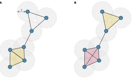
In Fig.5we provide examples of how different configurations on k and s can yield different connectivity structures for the same HOrS. If we allow any hyperedge or simplex dimension (s > 1) and any size of the intersection between

a b d c e h j a k i g f Face size Intersection A B C D Path connectivity

FIG. 5. Walks in HOrSs. Visualization of the different definitions of walks on an toy example of higher-order network. From left to right, the definition of the walk gets more restrictive. For each restriction on the defining variable of a walk (what elements are allowed to be considered for a walk and how much do they need to overlap in order to be adjacent)–we color what parts of the HOrS are reachable by at least a walk of length greater than one, and in gray what parts do not allow any walk to pass through them. In (C,D), some parts of the HOrS are connected only if the HOrS is a simplicial complex, and we visualize those with a striped pattern. We can see how the less restrictive walk (A), which can pass through two edges that have at least one vertex in common, yields the same connectivity as its underlying graph. Restricting the intersection between two adjacent edges to have at least 2 vertices in common, example (B), already highlights different mesoscale connectivity patterns in the HOrS, which can be further studied introducing a further restriction on the size of the edges, examples (C) and (D).

them (k > 0), then we find that all paths are valid and the whole toy HOrS is connected. In fact, we recover the simple graph connectedness (Fig.5A).

If we instead require that interactions share at least two vertices (k > 1), some paths are not allowed. For exam-ple, the triangle [2, 10, 12] is not connected to any of the triangles in the tetrahedron [1, 2, 3, 4], because the only intersection is 2.

Note also at this point that whether the HOrS is a hypergraph or a simplicial complex can make a difference. In Fig.5C, if we consider the HOrS to be a simplicial complex, the presence of the tetrahedron [1, 2, 3, 4] implies also the presence of all the subfaces. Combining this with the requirement k = 1, this also implies that some paths will not be walkable, e.g. all the triangles inside the tetrahedron share an edge with each other. Hence one cannot walk from one triangle to the other (shown as the black edges). However, there exist other paths that make the HOrS connected, for example, [1, 2, 4] is connected to [3, 4, 5]. Similar considerations also apply to Fig. 5D, which shows an example of the simplicial k-walk described earlier in this section, that is, a walk limited to jumps between lower adjacent simplices.

3. Eigenvector centralities

In some applications, it is important to quantify the influence of a node on the entire network, rather than its centrality relative to possible paths. First introduced in a sociological context by Bonacich [103], the eigenvector centrality tries to capture this effect using an iterative definition. In fact, the eigenvector centrality a node depends on the centrality of its neighbours [104]. In the graph case, it can be written as

xv= 1 λ_t∼v∑xt=

1

λ_t∈G∑avtxt (5)

where xvis the eigen-centrality of node v and avtthe adjacency matrix of the graph. Note that again the generalization to higher order interactions relies only on the definition of connectivity and paths. This measure has become widely used in a variety of situations ranging from Google’s PageRank [105] to neuron’s firing rate [106]. Interestingly, Bonacich [103] also showed that, if association is defined in terms of walks, a family of centralities can be defined

based on the length of walk considered. Degree centrality counts walks of length one, while eigenvalue centrality counts walks of length infinity. Alternative definitions of association are also reasonable. Alpha centrality allows vertices to have an external source of influence, while Estrada’s subgraph centrality proposes only counting closed paths (triangles, squares, etc) [94,101].

Bonacich [107] generalized eigenvector centrality to the case of bipartite graphs using their adjacency matrix. A feature of this definition is that one can compute centrality score for the same eigenvalue for both node sets. Using the same technique, one can compute eigenvalue centrality scores from incidence matrices for both hypergraphs, which will give an eigencentrality score for both vertices and hyperedges. A two-mode analysis of an incidence matrix then enables to identify central hyperedges in addition to nodes [108].

For motifs, it is possible to use the spectral features of the weighted motif adjacency matrix AM defined inIII A. For example, the clique motif eigenvector centrality score of node i is given by the ith component of the largest real eigenvector of W [109].

To incorporate non-linearities, we can make it so that the contribution of the centralities of two nodes in a 3-node hyperedge is multiplicative for the third. To do so, one can define the centrality using the eigenvector of the tensor Ak, where k labels the considered dimensions. There are several other types of tensor eigenvectors [110], and for this reason Benson [109] use Z- and H-eigenvectors which are arguably the most well-understood and commonly used tensor eigenvectors. The Z-eigenvector centrality vector is then defined as any positive vector c satisfying

T cm−1=λcm ∥c∥1=1 (6)

for some eigenvalue λ > 0 of the adjacency tensor T = Ak, and respectively the H-eigenvector centrality vector as the positive real vector c satisfying

T cm−1=λcm (7)

.

As we have seen before, for hypergraphs and simplicial complexes, adjacency can be defined not only at the vertex level, but also between hyperedges. It is possible to introduce notions of centralities for simplices and hyperedges through the components of the principal eigenvector of Ak [94]. The simplicial eigenvector centrality of the k-simplex α is given by the α component of the principal eigenvector of Ak, and its simplicial Katz centrality as Kk,α= [∑p=0∞xmAm_k ]αwhere 0 < x <_λ 1

1(Ak).

C. Triadic closure and clustering coefficient

A key concept in network analysis for going beyond node-related measures is triadic closure. It is a concept that comes from sociology [111], which argues that a strong social tie between two persons can only occur if it is part of a triangle. In other terms, my closest friends are the ones I share friends with. In a graph structure, triadic closure is represented as 2-paths of length 2 that are closed by an third edge. The fraction of pairs of neighbouring nodes that are themselves linked by an edge defines the node’s clustering coefficient. The clustering coefficient is an important network measure, which informs on the density of a node’s neighborhood. This coefficient can also be computed globally as the total percentage of 2-paths that are closed by and edge, i.e. are part of triangles.

This concept does not generalize well to bipartite graphs, because triangles - as any other odd cycle - do not exist in bipartite graphs. The global clustering coefficient can however be defined through its one-mode projections, as the number of 4-paths in the bipartite graph that are part of a 6-cycle [112,113].

Other attempts to generalize the concept of clustering coefficient beyond pairwise relations focused on keeping its close relation to the notion of triadic closure. One possibility is to define a local clustering coefficient from the new definitions of neighborhood that a node can have in a HOrS [114]. For example, in a simplicial complex, a neighborhood can also be defined at the maximal simplex level, and can also be defined for higher order simplices, not only for nodes [99].

Another possibility is to redefine the notion of paths [82] as sequence of vertices (v1, . . . , v`)such that two adjacent vertices vi, vi+1 both belong to the same hyperedge ei. Then, the clustering coefficient follows from its pairwise definition as the ratio of 2-paths that are closed by an edge. In a HOrS, paths can also be defined as sequence of k-cliques, or k − 1-simplices (e1, . . . , e`) such that two adjacent cliques ei, ei+1 have k − 1 nodes in common, which we will call k-paths as they are formed of k-cliques. In this case too, the clustering coefficient is then defined as the fraction of k-paths of length k that are part of a k + 1-clique [115].

In simplicial complexes, we can distinguish between a closed k-path of length k + 1 and a k-simplex. Hence, the clustering coefficient can be defined as the ratio of closed k-paths of length k + 1 that are closed by a k-simplex. In particular, when considering triangles, this definition of the clustering coefficient can be used to verify the sociological

intuition behind the diadic triadic closure idea [96], that is, it is possible to count how many actual “full” triangles (2-simplices) among the possible “empty” triangles constructed from three edges (a closed path of three 1-simplices). Finally, this higher-order clustering coefficient can be further generalized to motifs in weighted or growing HOrS [116].

D. Simplicial homology

One of the main reasons to use simplicial complexes as representations for higher-order datasets is a new algebraic toolset that studies the topology of the HOrS in a unique way: simplicial homology. Homology is an algebraic topological concept that enables us to study the structure of a simplicial complex at different dimensional scales. Before we can introduce homology, we need to define an algebraic structure on our simplicial complex. This requires imposing an orientation for each simplex in the complex, formalized as the ordering of the vertices. The orientation can be arbitrarily chosen, just like the choice of node labels in a network, and it is only needed in order to coherently perform the computations. An orientations is an equivalence class on the vertex orderings, where two orderings are equivalent if they differ by an even permutation [66, 117]. The orientation issue does not exist in a 0-simplex, since the nodes are not oriented, and only arises when we deal with higher order graphs. For simplicity, and with no loss of generality, we choose the orientation induced by the ordering of the vertex labels.

1. Boundary operators and homology groups

We can combine these oriented simplices in k−dimensional chains c = r1σ1+r2σ2+ ⋯where σi are k-dimensional simplices and ri ∈ _{F are coefficients in a field F. The collection of all possible k-chains in X is the vector space} Ck= {r1σ1+r2σ2+...∣ri∈_{F, σ}i∈Xk} where Xk is the set of k-simplices in X.

We can also define the dual space of Ck, denoted as the co-chain space, Ck as the linear space of all alternating functions f ∶ Ck → R. Chain and co-chain space are just two sides of the same coin, as they encode the same information. For instance, C1 can be interpreted as the space of edge-flow vectors and each of its elements f assigns a scalar to an edge, representing the intensity of flow along that edge with a sign which represent the agreement or not with the chosen orientation of the edge.

We can relate the k-chain space Ck to the k − 1 using the boundary operator, which maps each k-simplex to its k − 1-dimensional faces ∂k∶Ck→Ck−1. When applied on a simplex α = [v0, ..., vk], it gives:

∂k([v0, ..., vk]) = k ∑ i=0

(−1)i[v0, ...vi−1, vi+1, ..., vk]. (8)

Basically, in each term of the linear combination, we remove a vertex from the original simplex. In this way, we obtain its boundary as an alternate sum of the k − 1-order simplices. In a triangle [v0, v1, v2], for instance, we get the alternate sum of the three edges ([v1, v2] − [v0, v2] + [v0, v1]). The image of the boundary map, im(∂k), coincides with the space of (k − 1)-boundaries. The kernel ker(∂k)is instead the space of k-cycles, as it is easy to prove that for every cyclic chain c whose starting point coincides with the ending point ∂kc = 0. Moreover, ∂k○∂k+1=0, which implies that im(∂k+1) ⊆ker(∂k). The elements of ker(∂k)which are not included in im(∂k+1)can be denoted with the quotient space

Hk≡

ker(∂k) im(∂k+1)

(9) which takes the name of k-th homology group. The elements of Hk correspond to the k-cycles that are not induced by a k-boundary, namely the k-dimensional holes of our complex [66,117].

The dimension of the homology group Hk is called the k-th Betti number and it represents a way to classify the k-dimensional topology of a HOrS. Specifically, the 0th Betti number represents the number of connected component in the simplicial complex, the 1st Betti number is the number of cycles, the 2nd the number of voids enclosed by 2-dimensional simplices, 3rd the number of 4-dimensional voids etc.

2. Evolving simplicial complexes

Homology is an century old concept in algebra and is one the key tools for the study and classification of shapes in mathematics [117]. Recently the concept has been extended to weighted and growing simplicial complexes [118].