HAL Id: hal-01427439
https://hal-univ-tln.archives-ouvertes.fr/hal-01427439
Submitted on 5 Jan 2017
HAL is a multi-disciplinary open access
archive for the deposit and dissemination of
sci-entific research documents, whether they are
pub-lished or not. The documents may come from
teaching and research institutions in France or
abroad, or from public or private research centers.
L’archive ouverte pluridisciplinaire HAL, est
destinée au dépôt et à la diffusion de documents
scientifiques de niveau recherche, publiés ou non,
émanant des établissements d’enseignement et de
recherche français ou étrangers, des laboratoires
publics ou privés.
Second-Order Blind Source Separation: A New
Expression of Instantaneous Separating Matrix for
Mixtures of Delayed Sources
Gilles Chabriel-, Jean Barrère
To cite this version:
Gilles Chabriel-, Jean Barrère. Second-Order Blind Source Separation: A New Expression of
In-stantaneous Separating Matrix for Mixtures of Delayed Sources.
2006 IEEE 7th Workshop on
Signal Processing Advances in Wireless Communications , Jul 2006, Cannes, France.
pp.1 - 5,
�10.1109/SPAWC.2006.346397�. �hal-01427439�
SECOND-ORDER BLIND SOURCE SEPARATION: A NEW EXPRESSION OF
INSTANTANEOUS SEPARATING MATRIX FOR MIXTURES OF DELAYED SOURCES
Gilles Chabriel - Jean Barrère
STIC-TOULON/GESSY
Université du Sud Toulon-Var
Av. de l’Université, BP 20132
83162 LA GARDE Cedex (FRANCE)
Fax: (33) 494 142 598
[email protected] - [email protected]
ABSTRACT
In this paper, we study the blind separation of mixtures of propagating waves (delayed sources) encountered for ex-ample in underwater telephone (UWT) systems . We suggest a new second-order statistics method using as many observa-tions as sources. First, we show that each of theN delayed
sources can be developed as a particular linear combination of the different temporal-derivatives of theN observations.
Under some assumptions, an instantaneous rectangular sepa-rating matrix is then identified by the joint diagonalization of a set of covariance matrices estimated from the observations and its derivatives.
The algorithm used takes into account the particular structure of the spectral mixing matrix encountered.
A numerical simulation is provided in a 3-sources/3- observa-tions case for propagating audio signals.
1. INTRODUCTION
Consider a set ofN propagating waves sj(t) in an echo-free
and noise-free medium. These are recorded on a set ofM
identical sensors. Let xj(t) denote the contribution of the
sourcesj(t) on a sensor arbitrary indexed by 1, i.e. xj(t) is
a filtered version of the sourcesj(t). Assuming that the set
of sensors is sufficiently compact, then the contribution of the sourcesj(t) recorded on a sensor i is the same one as that
recorded on the first sensor, except for an attenuation factor and a propagation delay. The observationyi(t) recorded on
the sensori, is a linear combination of the delayed
contribu-tionsxj(t): y1(t) = N X j=1 xj(t), yi(t) = N X j=1 cijxj(t − τij), i ∈ [2, . . . , M ], (1) wherecijis the relative attenuation coefficient of sourcej on
sensori, and τij a relative propagation delay of sourcej on
sensori.
The different contributions are assumed to be band-limited, differently colored, statistically independent and zero-mean. Thereafter in the paper, the contributions will be called sources. The problem is to provide an estimation of theN different
sourcesxj(t) from the observations yi(t).
A first way to solve the problem using truncated Taylor se-ries of each delayed sourcexj(t − τij) has been successfully
treated in [1]-[5]. It consists of the estimate of an instanta-neous square mixing matrix MM ×M between the
observa-tions and the different derivatives of the sources:
[y1, y2, . . .]T = M [x1, x2, . . . , ˙x1, ˙x2, . . .]T.
For low delays, second-order statistics are sufficient to extract the different contributions from the observations (see [2], [4], [6]). For higher delays, a combination of two-order and high-order statistics methods is proposed in [3] to achieve the sep-aration.
The main limitation of these methods is the high necessary number of observations (up to several times the number of sources).
We propose here aN −sources N −sensors original approach
separating matrix S between the different derivatives of the observations and filtered sources:
£xh 1, x h 2, . . . x h N, ¤T
= S [y1, ˙y1, . . . , y2, ˙y2, . . . , yN, ˙yN, . . .] T
,
wherexh
j is the sourcexjfiltered by an invertible known filter
h.
It is important to note that the two approaches are not equiva-lent: the matrix M is not a simple pseudoinverse of S. The paper is organized as follows: in the next section we ex-plain how to construct the separating matrix S from the prop-agation model described by the system of equations (1). Then the third section explains the second-order statistics method implemented to estimate this separating matrix. The estima-tion uses a new version of the joint-diagonalizaestima-tion algorithm proposed by S.Dégerine in [7]. A description of this algo-rithm has to appear in english, a preprint can already be read in [8]. A numerical simulation in the last section illustrates the effectiveness of our approach.
2. EXPRESSION OF THE SEPARATING MATRIX
In the frequency domain, the system (1) becomes
Y1(ν) = N X j=1 Xj(ν), Yi(ν) = N X j=1 cije−2πντijXj(ν), i ∈ [2, . . . , N ]. (2)
Xj(ν) and Yi(ν) are respectively the Fourier Transforms (FT)
of thejthsource and of theithobservation.
The system (2) can be rewritten in matrix notation as:
Y(ν) = Mf(ν)X(ν), (3)
where
Y(ν) = [Y1(ν), . . . , YN(ν)]T, X(ν) = [X1(ν), . . . , XN(ν)]T.
TheN × N spectral mixing matrix Mf(ν) is defined as:
Mf(ν) = 1 . . . 1 c21e−2πντ21 . . . c2Ne−2πντ2N .. . . .. ... cn1e−2πντN 1 . . . cN Ne−2πντN N . (4)
We assume that Mf(ν) is regular for any frequency.
The inverse matrix of Mf(ν) is
Mf(ν)−1= 1
det Mf(ν)(adj M f(ν))T,
where adj Mf(ν) and det Mf(ν) are respectively is the
ad-joint matrix and the determinant of the matrix Mf(ν).
From equation (3), one has:
det Mf(ν) X(ν) = (adj Mf(ν))TY(ν). (5)
According to the particular structure of the spectral mixing matrix Mf(ν), its determinant (denoted by Hd(ν)) is a sum
of weighted complex exponentials:
Hd(ν) = det Mf(ν) =
X
i
βiexp(−2πντdi),
where the weightsβi are particular products of coefficients
cij, andτdi are particular sums of delaysτij.
Let H(ν) denote the transposed adjoint of M(ν). Each
en-triesHkl(ν) of H(ν) can also be expressed as a sum of weighted
exponentials:
Hkl(ν) = (adj Mf(ν))Tkl=
X
i
αkliexp(−2πντkli),
where the weightsαkliare also particular products of
coeffi-cientscij, andτkliare particular sums of delaysτij.
Back to the temporal representation, the system (5) becomes:
{hd∗ xk}(t) = N X l=1 {hkl∗ yl}(t), wherehkl(t) = FT−1(Hkl(ν)), hd(t) = FT−1(Hd(ν)) and
where{h.∗ x.}(t) =R h.(t − τ )x.(τ )dτ denotes the
convo-lution ofh.(t) and x.(t).
Each filtered source{hd∗ xk}(t) is then a finite sum of
de-layed observations:
{hd∗ xk}(t) =
X
l,i
αkliyl(t − τkli). (6)
Assuming that theτkliare “small” for all indices, yl(t − τkli)
can be approximated by its truncated up to P-order Taylor se-ries expansion. Each filtered source can be then approximated by a linear combination of the observations and its deriva-tives: {hd∗ xk}(t) ≈ X l,i αkli P X p=0 (−τkli)p p! y (p) l (t).
Fork = 1, . . . , N the system is rewritten as:
xh(t) ≈ S˜y(t), (7) where xh(t) = [xh
1(t), . . . , xhN(t)]
T is the filtered sources
vector, withxh
˜
y(t) = [y1, ˙y1, . . . , y1(P ), y2, . . . , y(P )2 , . . . , y (P ) N ]
T is the
ob-servations and their derivatives vector. S is theN × (N P + N ) separating matrix.
The analytical expression of each entry of S with respect to the parameterscijandτijis heavy but does not present
theo-retical difficulties. This expression is detailed in the Appendix A for the 2-sources/2-sensors case.
The joint estimation of the parameterscij,τijand of the
sepa-rating matrix S forms the basis of the iterative algorithm pro-posed in the following section.
3. PRESENTATION OF THE ALGORITHM
From (7) and because the sourcesxh
k(t) are mutually
uncorre-lated, it follows that S has to diagonalize the set of covariance matrices obtained at different lags Ry˜˜y(τk) =E{˜y(t)˜y
T(t +
τk)}:
SR˜y˜y(τk)ST = Λ(τk), ∀τk
Λ(τk) =E{xh(t)xhT(t+τk)} being a diagonal matrix
what-ever the lagτk.
S. Dégerine propose in [7],[8] a new algorithm (called Least Square on B or LSB) for approximate non-orthogonal joint diagonalization of a set of matrices. In its original form, this algorithm iteratively searches an optimal joint diagonalizer ˜S
of a set ofK matrices to the mean square sense. The
second-order criterion to be optimized is then
C(˜S) =X
k
Off(˜SR˜y˜y(τk)˜ST), (8)
where Off(.) is the sum of the square non diagonal elements
of the considered matrix. To perform the mean square opti-mization, S. Dégerine uses a relaxation on the lines of ˜S
con-ducting to solveN eigenvalue problems for each iteration.
Here, the expected diagonalizer S being non square, the opti-mization (8) does not conduct to an unique solution for ˜S. The
main idea is then to force the algorithm to hold the theoreti-cal structure of the separation matrix at each iteration. This theoretical expression depends on the parameterscij andτij.
At each step of relaxation, we estimate the parameterscijand
τijfrom their formal expression wrt the entries of the current
estimated ˜S. The next step is processed using an new ˜S built
on these estimated parameters.
An illustration of such theoretical expressions can be found in Appendices for the 2-sources case. For theN -sources case,
we implemented formal calculus subroutine in order to pro-vide automatically the formal expressions we need.
The final algorithm is summed up as follows:
Numerical Algorithm
1) From the observations y(t), build the observation
vectory(t) at the order P .˜
2) ComputeK covariance matrix Ry˜˜y(τk).
3) Intitialize ˜S(0) with arbitrary values.
4) Proceed to an iterationk with LSB algorithm.
5) From ˜S(k) obtained at step 4), estimate the attenuation
coefficientsck
ijand the propagation delaysτ k ij.
6) Fromck
ijandτijk, compute a new matrix ˜S(k + 1).
7) Repeat steps 4), 5) and 6) until the evolution of the estimated matrix ˜S becomes sufficiently weak.
4. RESULTS
We present now a numerical simulation in the 3-sources/3-observations case. The sources are 24s long music extracts. The sampling frequency isFs= 22.05kHz.
The matrix C of relative attenuations is:
C= 1.0000 1.0000 1.0000 2.0000 1.3000 1.2000 3.0000 1.6000 2.2000 .
The matrix D of relative propagation delays is:
D= 0 0 0 30.00µs 18.00µs 5.00µs 25.00µs 12.50µs 10.00µs .
For the 3 observations, we take a Taylor series expansion up to 3-order (P = 3). 151 covariance matrices Ry˜˜y(τk) are
used (K = 151), with τk = k/F s, k ∈ {−75, 75}.
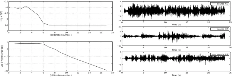
Fig. 1 (a) shows the evolution of the optimization criterion
C(˜S) at each iteration number i and part (b) presents the
0 2 4 6 8 10 12 14 16 18 −3 −2.5 −2 −1.5 −1 −0.5
(a) Iteration number i
Log of C(S) 0 2 4 6 8 10 12 14 16 18 −20 −15 −10 −5 0 (b) Iteration number i Log of Norm(S(i+1)−S(i)) Fig. 1. Convergence
After convergence (8 iteration steps), we obtain the fol-lowing estimations for the relative attenuations and for the relative propagation delays:
˜ C= 1.0000 1.0000 1.0000 1.9995 1.3047 1.1967 2.9998 1.6053 2.1929 , ˜ D= 0 0 0 31.64µs 18.87µs 5.03µs 26.56µs 13.13µs 9.81µs .
Taking the matrices ˜C and ˜D into account, the filterHd(ν)
can be identified and its effect reversed after separation. We obtain the following source estimations (Fig. 2) that have to be compared to the original ones (Fig. 3).
0 5 10 15 20 25 −4 −2 0 2 4 Time (s) estimated source #1 0 5 10 15 20 25 −10 −5 0 5 10 Time (s) estimated source #2 0 5 10 15 20 25 −10 −5 0 5 Time (s) estimated source #3
Fig. 2. Estimated sources
0 5 10 15 20 25 −4 −2 0 2 4 Time (s) source #1 0 5 10 15 20 25 −10 −5 0 5 10 Time (s) source #2 0 5 10 15 20 25 −10 −5 0 5 Time (s) source #3
Fig. 3. Original sources
The mean square errors (MSE) between the estimated sources and the original ones and the corresponding Signal to Interfer-ence Ratio (SIR) are presented in the Table 1.
source #1 source #2 source #3
MSE 0.0141 0.0155 0.0164
SIR 41 dB 44 dB 36 dB
Table 1. Performances
5. CONCLUSION
This paper present a novel iterative method for blind source separation from delayed mixtures. The delayed mixtures are approached by instantaneous mixtures of the observation deriva-tives. This approach uses only second-order statistics and needs no more mixtures than sources. The algorithm is based on the joint diagonalization of a set of spatial covariance ma-trices but the non square separating matrix is constrained to hold a theoretical structure at each iteration. A numerical sim-ulation shows the efficiency of the approach.
APPENDIXA
FROMMf(ν)TOSIN THE2-OBSERVATIONS CASE.
Now, we have the following spectral mixing matrix
Mf(ν) = · 1 1 c21e−2πντ21 c22e−2πντ22 ¸ . (9)
In this case (6) leads to the 2 following filtered sources:
xh 1(t) = c22y1(t − τ22) − y2(t), xh 2(t) = −c21y1(t − τ21) + y2(t), wherexh k(t) = xk(t − τ22) − xk(t − τ21), k ∈ [1, 2].
With xh(t) = [xh
1, xh2]T, andy˜(t) = [y1, ˙y1, ¨y1, . . . , y(P )1 , y2]T,
the(2 × P + 2) unmixing matrix of equation (7) becomes:
S= " c22 −c22τ22 . . . c22(−τ22) P P! −1 −c21 c22τ21 . . . −c21(−τ21) P P! 1 # . APPENDIXB
FROMSTOcij, τij IN THE2-OBSERVATIONS CASE.
Here, we have the following separating matrix
S= · s11 s12 . . . s1P s1P +1 s21 s22 . . . s2P s2P +1 ¸ ,
one has the(2 × 2) spectral separating matrix
Sf(ν) = · sf11(ν) s f 12(ν) sf21(ν) s f 22(ν) ¸ ,
where the entries of Sf(ν) are polynomials in ν:
sf11(ν) = PP k=1(2jπν) ks 1k, sf12(ν) = s1P +1, sf21(ν) = PP k=1(2jπν)ks2k, sf22(ν) = s2P +1.
The inverse matrix of Sf(ν) is also a matrix of polynomials: £Sf(ν)¤−1 = 1 det Sf(ν) · p11(ν) p12(ν) p21(ν) p22(ν) ¸ .
An approximation of the spectral mixing matrix Mf(ν) is
obtained normalizing each column of the previous matrix by
p1k(ν) Mf(ν) ≈ · 1 1 p21(ν)/p11(ν) p22(ν)/p12(ν) ¸ .
The entries of the second line of this matrix can be developed in power series expansion inν:
p21(ν)/p11(ν) = q0+ q1ν + O2(ν),
p22(ν)/p12(ν) = r0+ r1ν + O2(ν).
Identifying these expansions with the Taylor-series expansion of the entries of Mf(ν) (see 9) we find:
c21 = q0, τ21 = − 1 j2π q1 q0 , c22 = r0, τ22 = − 1 j2π r1 r0 . 6. REFERENCES
[1] G. Chabriel and J.Barrère, Blind Identification of Slightly
Delayed Mixtures, in Proc. of the Tenth IEEE Workshop
on Statistical Signal and Array Processing, pp. 319-323, August 14-16, 2000.
[2] J. Barrère and G. Chabriel, A Compact Sensor Array for
Blind Separation of Sources, IEEE Trans. on Circuits and
Systems, Part I, Vol. 49, No 5, pp. 565-574, May 2002. [3] G. Chabriel and J. Barrère, An Instantaneous Formulation
of Mixtures for Blind Separation of Propagating Waves,
IEEE Trans. on Signal Processing, Vol. 54, No. 1, pp.49-58 Jan. 2006.
[4] G. Cauwenberghs, M. Stanacevic and G. Zweig, Blind
Broadband Source Localization and Separation in Minia-ture Sensor Arrays in Proc. of IEEE Int. Symp. Circuits
and Systems (ISCAS’2001), Vol. 3, pp. 193-196, Sydney, Australia, 2001.
[5] A. Yeredor, Blind Source Separation with Pure Delay
Mixtures, in Proc.2ndInternational Symposium on
In-dependent Component Analysis and Blind Signal Separa-tion (ICA’2001), pp. 691-696, December 2001, San diego - California, USA.
[6] M. Stanacevic and G. Cauwenberghs, Micropower
Gra-dient Flow VLSI Acoustic Localizer in IEEE Transactions
on Circuits and Systems I : Regular Papers, to appear, 2005.
[7] S. Dégerine, Sur la diagonalisation conjointe approchée
par un critère des moindres carrés, in Proc. of the18e
Colloque GRETSI sur le traitement du signal et des im-ages, pp. 311-314, Toulouse 2001.
[8] Serge Dégerine and Elimane Kane, A new non-orthogonal approximate joint diag-onalization algorithm for blind source sep-aration, in http://www-lmc.imag.fr/lmc-sms/Serge.Degerine/Publications/LSBr.pdf