Supplemental Information Altering the Temporal Regulation of One Transcription Factor Drives Evolutionary Trade-Offs between Head Sensory Organs

(1)

Developmental Cell, Volume50

Supplemental Information

Altering the Temporal Regulation of One

Transcription Factor Drives Evolutionary

Trade-Offs between Head Sensory Organs

Ariane Ramaekers, Annelies Claeys, Martin Kapun, Emmanuèle Mouchel-Vielh, Delphine Potier, Simon Weinberger, Nicola Grillenzoni, Delphine Dardalhon-Cuménal, Jiekun Yan, Reinhard Wolf, Thomas Flatt, Erich Buchner, and Bassem A. Hassan

(2)

Supplemental Information

Altering the temporal regulation of one transcription factor drives

evolutionary trade-offs between head sensory organs

Ariane Ramaekers, Annelies Claeys, Martin Kapun, Emmanuèle Mouchel-Vielh, Delphine Potier, Simon Weinberger, Nicola Grillenzoni, Delphine Dardalhon-Cuménal, Jiekun Jan, Reinhard Wolf, Thomas Flatt,Erich Buchner, Bassem A. Hassan

Figure S1, Related to Figure 1

Figure S2, Related to Figures 1, 4, 6

Figure S4, Related to Figures 3, 4

Figure S6, Related to Figures 4, 6, S5

Table S1, Related to Figures 1, S1

Table S2, Related to Figure 4

Tables S3 and S4, Related to Figure 5

(3)

Figure S1. Natural variation in eye size in Drosophila, Related to Figure 1

(A to C’) Eye size comparison between females from five Drosophila species: D. melanogaster (D. mel.), D. yakuba (D. yak.), D. ananassae (D.ana.), D. pseudoobscura (D. pse.), D. virilis (D. vir.). Different numbers indicate different strains (see Methods). Boxes indicate interquartile ranges, lines medians and whiskers data ranges.

(A) Phylogenic relationship between the five species (tree branches are not scaled). (B) Eye: Face ratio measured from SEM images.

(C) Ommatidia number counted on SEM images. Ordinary one-way ANOVA **** p<0.0001 followed by Dunnett’s multiple comparisons. See also Table S1.

(D) Ommatidia width. Ordinary one-way ANOVA **** p<0.0001 followed by Dunnett’s multiple comparisons. See also Table S1

(4)

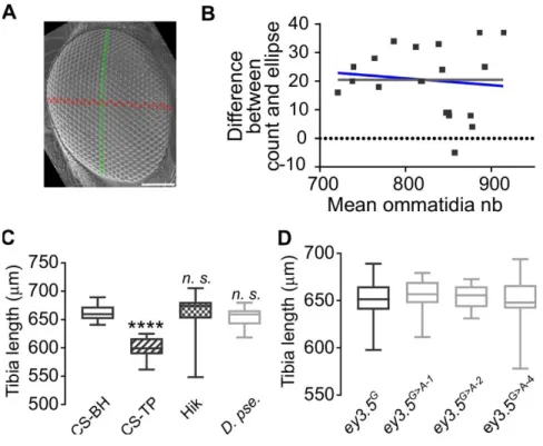
Figure S2. Ommatidia number variation: scaling and methods, Related to Figures 1, 4 and 6

(A) SEM image of a D. mel. Hikone-AS eye. Green: dorso-ventral axis; Red: anterior-posterior axis. Scale bar: 100 m.

(B) Bland-Altman chart plotting the difference in ommatidia number measured by two methods (ellipse-based estimation vs direct counting) over their mean (Bland and Altman, 1986). Comparison of fits indicates that the difference between the two measurements is independent of the mean (null hypothesis, grey line: slope= 0.0; alternative hypothesis blue line: slope unconstrained = -0.02372; p=0.6212).

(C) Mesothoracic tibia (T2) length in three wild-type D. mel. stocks (Canton-SBH_{, Canton-S}TP_{, Hikone-AS)}

and D. pse..

Sample sizes from left to right (n=21, n=23, n=29, n=21). Kruskal Wallis test **** p<0.0001 followed by Dunn’s multiple comparisons: **** p<0.0001; n.s. p>0.9999.

(D) Mesothoracic tibia (T2) length in CRISPR/Cas9 engineered and control lines. Sample sizes (n=20). Ordinary One way ANOVA n.s. p=0.7600.

(5)

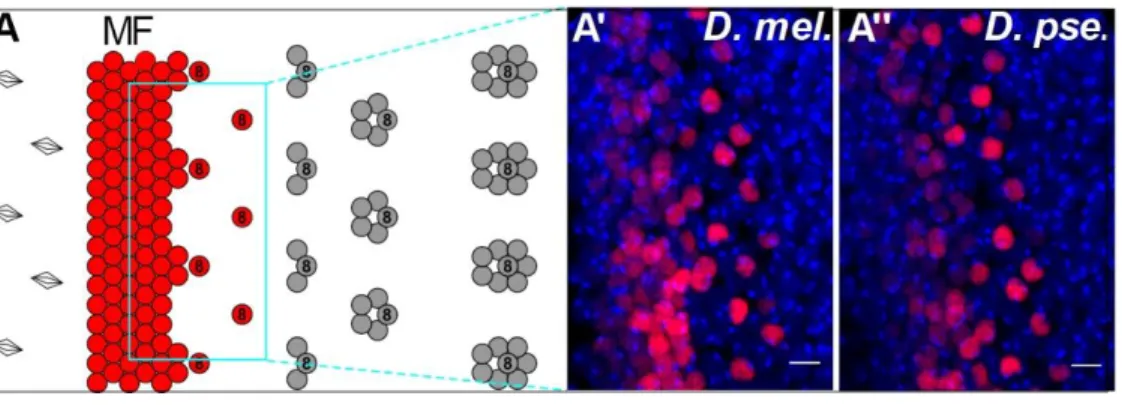
Figure S3. Developmental origin of eye size variation in D. mel. and D. pse., Related to Figure 2

(A) Schematics of the first steps of retinal differentiation showing the singling-out of committed Ato-expressing R8 ommatidia progenitor cells and subsequent steps of ommatidia assembly. (A’ and A’’) The density of Ato-expressing R8 progenitors (in red in A’ and A’’) is similar in the two species. Red: anti-Ato immunostaining; blue: DAPI. Anterior is at the left. Scale bars: 5 m.

(6)

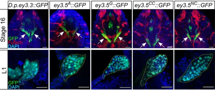
Figure S4. Eyeless enhancer activity in early EADs. Related to Figure 3 and Figure 4.

The D. pse. and the four D. mel. alleles of the ey eye enhancer drive GFP expression in the entire EAD in stage 16 embryos (arrows in upper panel) and in 1st instar larvae (L1; yellow dashed line in lower panel). Green: GFP; Blue: DAPI; Red: anti-Futsch (22C10). Scale bars: 20 m.

(7)

(8)

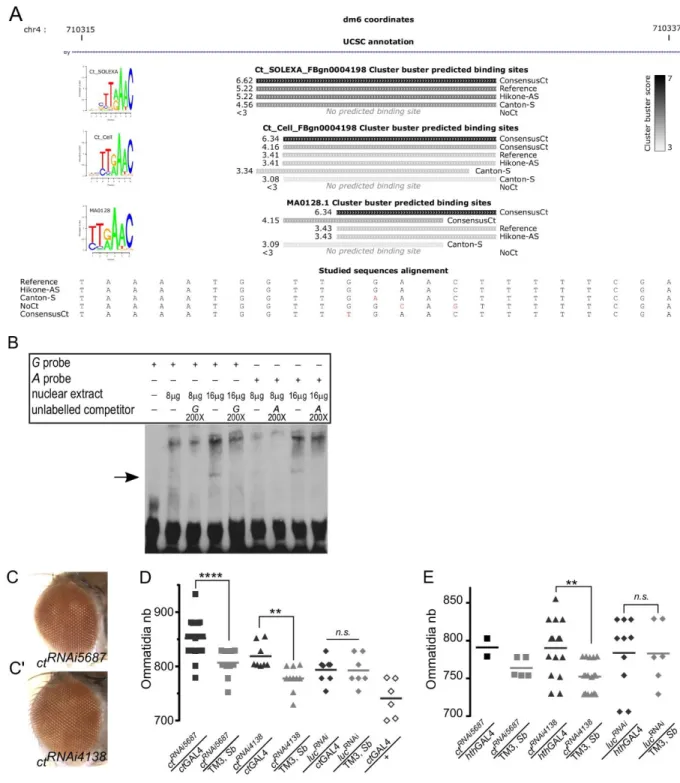
(A) Visualization of Cluster-Buster Ct predicted binding sites for natural and synthetic ey enhancer alleles at the SNP location. Scores are represented by a grey scale. PWMs corresponding sequence logos plotted by seqLogo (https://rdrr.io/bioc/seqLogo/) are shown on the left.

(B) Electrophoretic mobility shift assay. The Cut-FLAG nuclear extract induces a band shift (black arrow) with oligonucleotide probes corresponding to both G and A-enhancer alleles. Both shifts are eliminated when corresponding non-labeled competitors are added.

(C and C’) RNAi-mediated KD of ct using two distinct RNAi constructs does not induce gross morphology defects in the compound eye. Gal4 driver: ctGal4.

(D) Overexpression of two UAS-ctRNAi and one UAS-luciferaseRNAi constructs under the control of ctGAL4. Sample sizes from left to right (n=23, n=13, n=8, n=10, n=8, n=7, n=6). Ordinary one-way ANOVA **** p<0.0001 followed by Sidak’s multiple comparisons: ctRNAi5687/ctGal4 vs ctRNAi5687/ TM3, Sb **** p<0.0001; ctRNAi5687/ctGal4 vs ctGAL4/ + **** p<0.0001; ctRNAi4138_{/ctGal4 vs ct}RNAi4138_{/TM3, Sb * p=0.0126; ct}RNAi4138_{/ctGal4 vs ctGAL4/ + **** p<0.0001;}

lucRNAi /ctGal4 vs lucRNAi / TM3, Sb n. s. p>0.9999; lucRNAi /ctGal4 vs ctGAL4/ + ** p=0.0036. (E) Overexpression of two UAS-ctRNAi and one UAS-luciferaseRNAi constructs under the control of hthGAL4. Sample sizes, from left to right (n=2, n=5, n=15, n=17, n=10, n=7). Sample size for ctRNAi5687/hthGAL4 was low due to the lethality or gross morphological defects caused by this allelic combination. Ordinary one-way ANOVA ** p=0.0089 followed by Sidak’s multiple comparisons: ctRNAi4138/hthGal4 vs ctRNAi4138/TM3, Sb ** p=0.0047; lucRNAi /hthGal4 vs lucRNAi / TM3, Sb n. s. p=0.2152.

(9)

(10)

Figure S6. Eye: Face ratio, absolute A3 width and absolute face width. Related to Figure 4, Figure 6 and Figure S5.

Boxes indicate interquartile ranges, lines medians and whiskers data ranges.

(A) Sample sizes (n=12, n=14, n=10). Ordinary one-way ANOVA **** p<0.0001 followed by Tukey’s multiple comparisons: **** adjusted p<0.0001.

(A’) Sample sizes (n=11, n=11, n=13). Ordinary one-way ANOVA ** p=0.0035 followed by Tukey’s multiple comparisons: ** adjusted p=0.0043; * adjusted p = 0.0184; n.s adjusted p=0.7600.

(A’’) Sample sizes (n=12, n=14, n=10). Ordinary one-way ANOVA **** p<0.0001 followed by Tukey’s multiple comparisons: **** adjusted p<0.0001.

(B) Sample sizes (n=19, n=19, n=12, n=12). Unpaired t-tests: **** p<0.0001; n.s. p=0.37831. (B’) Sample size (n=12). Unpaired t-tests: * p=0.0288; * p=0.0444.

(B’’) Sample sizes (n=13, n=13, n=12, n=12). Unpaired t-tests: ** p=0.0042; * p=0.0163. (C) Sample size (n=42). Unpaired t-tests: ** p=0.0060.

(C’) Sample sizes (n=16, n=14). Unpaired t-tests: n.s. p=0.0553. (C’’) Sample size (n=42). Unpaired t-tests: n.s. p=0.5831. (D) Sample sizes (n=9; n=16). Unpaired t-tests: n.s. p=0.2625. (D’) Sample sizes (n=9; n=16). Unpaired t-tests: n.s. p=0.2220. (D’’) Sample sizes (n=9; n=16). Unpaired t-tests: n.s. p=0.5353.

(E) Estimated ommatidia numbers in control G-carrying and the four CRISPR engineered A-carrying variants imaged by light microscopy. Sample sizes: from left to right (n=24, n=8, n=32, n=33, n=45); Ordinary one-way ANOVA *** p=0.0009 followed by Dunnet’s multiple comparisons between the control and the four CRISPR lines.

(11)

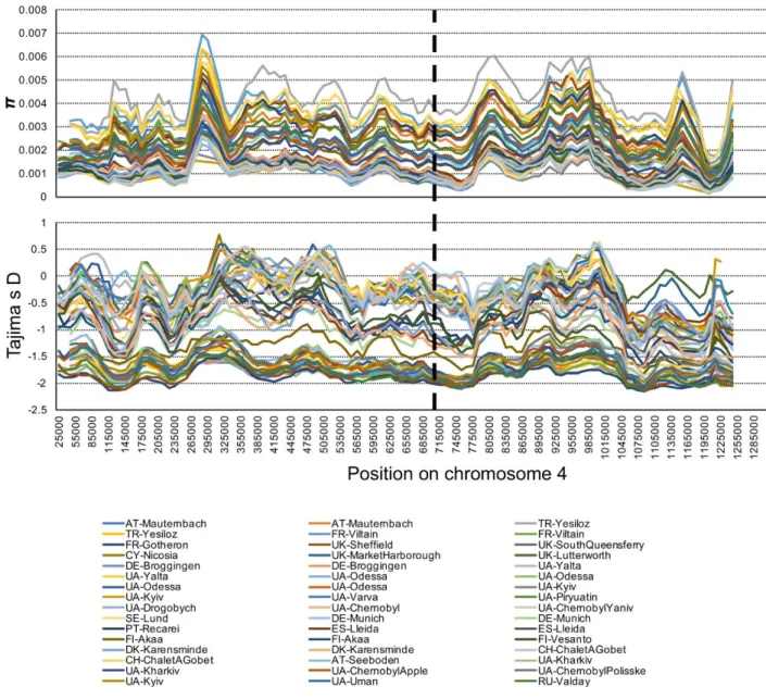
Figure S7. Genetic variation of the fourth chromosome in Europe, Related to Figure 5

The distribution of π (top panel) and Tajima’s D (bottom panel) in 50kb windows with 10kb step-size for 48 population samples from Europe. The vertical dashed black line indicates the approximate genomic position of the focal SNP at position Chr 4: 710326.

(12)

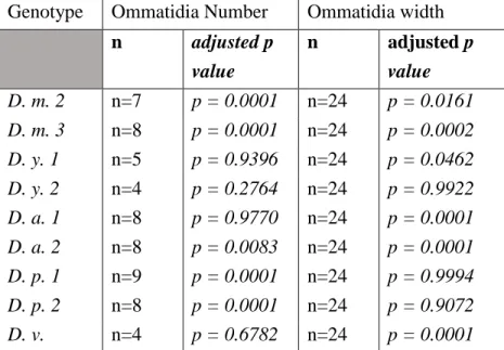
Table S1. Natural variation in Drosophila eye size, Related to Figures 1, S1.

Sample sizes and results of Dunnett’s multiple comparison tests following ordinary one-way ANOVA from Figure S1. Comparisons towards D. m. 1 (Canton-SBH_{; ommatidia number sample} size n=6; ommatidia width sample sizes n=24).

Genotype Ommatidia Number Ommatidia width

n adjusted p value n adjusted p value D. m. 2 n=7 p = 0.0001 n=24 p = 0.0161 D. m. 3 n=8 p = 0.0001 n=24 p = 0.0002 D. y. 1 n=5 p = 0.9396 n=24 p = 0.0462 D. y. 2 n=4 p = 0.2764 n=24 p = 0.9922 D. a. 1 n=8 p = 0.9770 n=24 p = 0.0001 D. a. 2 n=8 p = 0.0083 n=24 p = 0.0001 D. p. 1 n=9 p = 0.0001 n=24 p = 0.9994 D. p. 2 n=8 p = 0.0001 n=24 p = 0.9072 D. v. n=4 p = 0.6782 n=24 p = 0.0001

(13)

Table S2. Ct binding site predictions at the SNP location, Related to Figure 4

Data are presented in a separate Excel document.

Predictions of Ct binding sites in a 1 kb region surrounding the SNP at position Chr 4: 710326 (500 bp up and down) scored with Cluster-Buster (Frith et al., 2003).

(14)

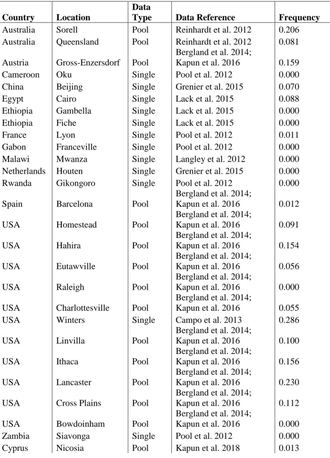
Table S3. Worldwide allele frequency patterns, Related to Figure 5

Country Location

Data

Type Data Reference Frequency

Australia Sorell Pool Reinhardt et al. 2012 0.206

Australia Queensland Pool Reinhardt et al. 2012 0.081 Austria Gross-Enzersdorf Pool

Bergland et al. 2014;

Kapun et al. 2016 0.159

Cameroon Oku Single Pool et al. 2012 0.000

China Beijing Single Grenier et al. 2015 0.070

Egypt Cairo Single Lack et al. 2015 0.088

Ethiopia Gambella Single Lack et al. 2015 0.000

Ethiopia Fiche Single Lack et al. 2015 0.000

France Lyon Single Pool et al. 2012 0.011

Gabon Franceville Single Pool et al. 2012 0.000

Malawi Mwanza Single Langley et al. 2012 0.000

Netherlands Houten Single Grenier et al. 2015 0.000

Rwanda Gikongoro Single Pool et al. 2012 0.000

Spain Barcelona Pool

Kapun et al. 2016 0.012

USA Homestead Pool

Kapun et al. 2016 0.091

USA Hahira Pool

Kapun et al. 2016 0.154

USA Eutawville Pool

Kapun et al. 2016 0.056

USA Raleigh Pool

Kapun et al. 2016 0.000

USA Charlottesville Pool

Kapun et al. 2016 0.055

USA Winters Single Campo et al. 2013 0.286

USA Linvilla Pool

Kapun et al. 2016 0.100

USA Ithaca Pool

Kapun et al. 2016 0.156

USA Lancaster Pool

Kapun et al. 2016 0.230

USA Cross Plains Pool

Kapun et al. 2016 0.112

USA Bowdoinham Pool

(15)

Turkey Yesiloz Pool Kapun et al. 2018 0.000

Turkey Yesiloz Pool Kapun et al. 2018 0.019

Portugal Recarei Pool Kapun et al. 2018 0.034

Spain Lleida Pool Kapun et al. 2018 0.000

Spain Lleida Pool Kapun et al. 2018 0.029

Ukraine Yalta Pool Kapun et al. 2018 0.000

France Gotheron Pool Kapun et al. 2018 0.128

Ukraine Odessa Pool Kapun et al. 2018 0.000

Switzerland ChaletAGobet Pool Kapun et al. 2018 0.096 Switzerland ChaletAGobet Pool Kapun et al. 2018 0.081

Austria Seeboden Pool Kapun et al. 2018 0.055

Germany Munich Pool Kapun et al. 2018 0.045

Germany Munich Pool Kapun et al. 2018 0.021

Germany Broggingen Pool Kapun et al. 2018 0.052

Germany Broggingen Pool Kapun et al. 2018 0.090

Austria Mauternbach Pool Kapun et al. 2018 0.053

Austria Mauternbach Pool Kapun et al. 2018 0.029

Ukraine Uman Pool Kapun et al. 2018 0.000

France Viltain Pool Kapun et al. 2018 0.029

France Viltain Pool Kapun et al. 2018 0.131

Ukraine Drogobych Pool Kapun et al. 2018 0.000

Ukraine Kharkiv Pool Kapun et al. 2018 0.000

Ukraine Piryuatin Pool Kapun et al. 2018 0.000

Ukraine Kyiv Pool Kapun et al. 2018 0.000

Ukraine Varva Pool Kapun et al. 2018 0.000

Ukraine ChernobylApple Pool Kapun et al. 2018 0.020

Ukraine

ChernobylPolissk

e Pool Kapun et al. 2018 0.015

Ukraine Chernobyl Pool Kapun et al. 2018 0.000

Ukraine ChernobylYaniv Pool Kapun et al. 2018 0.036

UK Lutterworth Pool Kapun et al. 2018 0.078

UK

MarketHarboroug

h Pool Kapun et al. 2018 0.072

(16)

Sweden Lund Pool Kapun et al. 2018 0.121

Denmark Karensminde Pool Kapun et al. 2018 0.019

Denmark Karensminde Pool Kapun et al. 2018 0.000

UK SouthQueensferry Pool Kapun et al. 2018 0.173

Russia Valday Pool Kapun et al. 2018 0.000

Finland Akaa Pool Kapun et al. 2018 0.048

Finland Akaa Pool Kapun et al. 2018 0.018

Finland Vesanto Pool Kapun et al. 2018 0.000

Origin, data type, data source and allele frequencies of the A-variant of the focal SNP at position Chr 4: 710326 of world-wide populations with sample sizes ≥ 10 individuals.

(17)

Table S4. Isofemale line genotypes, Related to Figure 5

Data are presented in a separate Excel document.

(18)

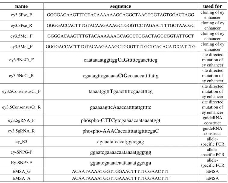
Table S5. List of oligonucleotides, Related to Star Methods

name sequence used for

ey3.3Pse_F GGGGACAAGTTTGTACAAAAAAGCAGGCTAAGTGGTAGTGGACTAGG cloning of ey

enhancer

ey3.3Pse_R GGGGACCACTTTGTACAAGAAAGCTGGGTCCTAGAATTTTGCTAACGC cloning of ey

enhancer

ey3.5Mel_F GGGGACAAGTTTGTACAAAAAAGCAGGCTGGACTAGGCGGTATTGCT cloning of ey

enhancer

ey3.5Mel_F GGGGACCACTTTGTACAAGAAAGCTGGGTTTTGCTCACACATCCATTTG cloning of ey

enhancer ey3.5NoCt_F caataaaatggttggCaGtttttcgaactttcg site directed mutation of ey enhancer ey3.5NoCt_R cgaaagttcgaaaaaCtGccaaccattttattg site directed mutation of ey enhancer ey3.5ConsensusCt_F taaaatggttTgaactttttcgaactttcg site directed mutation of ey enhancer ey3.5ConsensusCt_R gaaaaagttcAaaccattttattgttttc site directed mutation of ey enhancer

ey3.5gRNA_F phospho-CTTCgtcgaaaacaataaaatggt guideRNA _construct

ey3.5gRNA_R phospho-AAACaccattttattgttttcgaC guideRNA _construct

ey_R3 agaaatatcacatggccgag _{specific PCR}

allele-ey-SNPG-F ggaatcgaaaacaataaaatggctgg _{specific PCR}

allele-Ey-SNPA_-F _{ggaatcgaaaacaataaaatggctga}

allele-specific PCR

EMSA_G ACAATAAAATGGTTGGAACTTTTTCGAACTTT EMSA