HAL Id: tel-01274065
https://hal.archives-ouvertes.fr/tel-01274065
Submitted on 15 Feb 2016HAL is a multi-disciplinary open access archive for the deposit and dissemination of sci-entific research documents, whether they are pub-lished or not. The documents may come from teaching and research institutions in France or abroad, or from public or private research centers.
L’archive ouverte pluridisciplinaire HAL, est destinée au dépôt et à la diffusion de documents scientifiques de niveau recherche, publiés ou non, émanant des établissements d’enseignement et de recherche français ou étrangers, des laboratoires publics ou privés.
Public Domain
Multidimensionnelles
Sofian Maabout
To cite this version:
Sofian Maabout. Contributions à l’Optimisation de Requêtes Multidimensionnelles. Databases [cs.DB]. Université de Bordeaux, 2014. �tel-01274065�
Habilitation à Diriger des Recherches
UNIVERSITÉ DE BORDEAUX
École doctorale de Mathématiques et Informatique de Bordeaux DOMAINE DE RECHERCHE : Informatique
Présentée par
Sofian Maabout
Contributions à l’Optimisation de Requêtes
Multidimensionnelles
Soutenue le 12 Décembre 2014
Devant le jury composé de
Mme. Christine Collet Professeur à l’INP de Grenoble Rapporteur
M. Nicolas Hanusse Directeur de Recherche au CNRS Examinateur
M. Yves Métivier Professeur à Bordeaux INP Examinateur
M. Jean-Marc Petit Professeur à l’INSA de Lyon Rapporteur
M. Pascal Poncelet Professeur à l’Université Montpellier 2 Rapporteur M. Philippe Pucheral Professeur à l’Université de Versailles Saint-Quentin Examinateur M. David J. Sherman Directeur de Recherche à INRIA Bordeaux Sud-Ouest Examinateur
1 Introduction Générale 1
2 Calcul Parallèle de Bordures et Applications 5
2.1 Introduction . . . 5
2.2 Basic Concepts Related to MFI’s . . . 6
2.3 Related Work w.r.t MFI’s Mining . . . 7
2.4 Basic Definitions . . . 9
2.4.1 Pure Depth Traversal . . . 10
2.5 MineWithRounds Algorithm . . . 11
2.6 Data Distribution . . . 15
2.7 MFI’s Mining Experiments . . . 16
2.7.1 OpenMP . . . 16
2.7.2 Machine . . . 16
2.7.3 Data sets. . . 16
2.7.4 Results Analysis . . . 18
2.7.5 MineWithRounds vs PADS . . . 20
2.8 Concluding Remarks on MFI’s Computation . . . 23
2.9 Parallel Mining of Dependencies . . . 23
2.10 Related Work w.r.t Mining Functional Dependencies . . . 24
2.11 Basic Definition w.r.t Dependencies . . . 25
2.11.1 Functional dependencies . . . 25
2.11.2 Keys . . . 26
2.11.3 Conditional Functional Dependencies . . . 26
2.11.4 Problems statement . . . 27
2.12 Mining Minimal Keys . . . 27
2.13 Mining Functional Dependencies . . . 30
2.13.1 Distinct Values Approximation . . . 31
2.14 Mining Conditional Functional Dependencies . . . 32
2.15 Dependencies Mining Experiments . . . 33
2.15.1 Exact FDs . . . 33
2.15.2 Approximating FDs . . . 36
Table des matières
3 Optimisation des requêtes dans les cubes de données 39
3.1 Preliminaries . . . 39
3.1.1 Problem Statement . . . 43
3.1.2 Related Work . . . 43
3.2 PickBorders . . . 44
3.3 Workload optimization . . . 46
3.3.1 View Selection as Minimal Weighted Vertex Cover . . . 46
3.3.2 Exact Solution . . . 47
3.3.3 Approximate Solution . . . 47
3.3.4 Reducing the Search Graph . . . 48
3.4 Dynamic Maintenance . . . 49
3.4.1 Stability . . . 49
3.5 Some Connections with Functional Dependencies . . . 50
3.6 Experiments . . . 51
3.6.1 Cost and memory . . . 51
3.6.2 Performance factor . . . 52
3.6.3 Stability Analysis . . . 56
3.7 Conclusion and Future Work . . . 57
4 Optimisation des requêtes skyline 59 4.1 Introduction . . . 59
4.2 Preliminaries . . . 61
4.3 Partial Materialization of Skycubes . . . 62
4.3.1 Properties of Subspace Skylines . . . 63
4.3.2 The Interplay Between FDs and Skylines . . . 65
4.3.3 Analysis of the number of closed subspaces . . . 66
4.3.4 Skyline size analysis . . . 67
4.3.5 Data Dynamics . . . 68
4.3.6 Computing the Closed Subspaces . . . 69
4.4 Query evaluation . . . 70
4.4.1 Full Materialization . . . 72
4.5 Related Work . . . 73
4.6 Experiments . . . 74
4.6.1 Full Skycube Materialization . . . 75
4.6.2 Storage Space Analysis . . . 78
4.6.3 Query Evaluation . . . 81
4.7 Conclusion and Future Work . . . 82
5 Conclusion générale 85
Introduction Générale
L’analyse mutidimensionnelle des données est un sujet vase qui va des statistiques avec des tech-niques telles que l’analyse en composantes principales au calcul haute performance en passant par l’extraction de connaissances via du clustering ou la classification, les bases de données, l’algorith-mique et les techniques d’approximation.
Nos contributions à l’analyse multidimensionnelle suivent la même démarche, à savoir : Nous considérons un type particulier d’analyse, dans la terminologie bases de données nous parlons de requête multidimensionnelle, et nous proposons des solutions d’optimisation. En général, il s’agit de minimiser le temps d’exécution de l’analyse. Mais pas seulement. En effet, certaines requêtes sont gourmandes en mémoire. Ainsi, un deuxième critère que nous tentons d’optimiser est la consomma-tion mémoire.
Notre démarche pour ce faire consiste à exploiter autant que faire se peut l’infrastructure ma-térielle à disposition notamment par la disponibilité de plusieurs unités de calcul. En effet, même les ordinateurs portables sont actuellement équipés de plusieurs processeurs. Ainsi, l’algorithmique parallèle n’est plus un luxe réservé à quelques centres de calcul de grands organismes de recherche. A titre d’exemple, en 2013 une machine avec 12 processeurs et une mémoire de 64 Go peut être achetée à moins de 5KE.
Certains problèmes sont théoriquement prouvés qu’ils sont difficiles. N’empêche qu’en pratique, la pire des situations est rarement atteinte et avec de bonnes heuristiques et des astuces de program-mation, l’on arrive a résoudre des instances de grandes tailles. L’exemple notoire est le problème SAT qui est en quelque sorte l’étalon des problèmes NP-Complets et qui malgré tout continue à susciter des avancées, théoriques et pratiques, qui permettent actuellement d’envisager de résoudre des instances à plusieurs millions de variables. Nos travaux tiennent compte de ce fait d’où le soucis d’accompagner à chaque fois l’analyse théorique d’expérimentations permettant si ce n’est de valider l’approche, du moins d’en donner un aperçu sur son potentiel.
Un troisième axe que nous considérons est celui ayant trait à l’algorithmique approché. En effet, dans plusieurs applications pratiques, un résultat approché (avec cependant une marge d’erreur maîtrisée) est largement suffisant du moment que ce dernier peut être obtenu avec une complexité acceptable. Ceci est d’autant plus vrai quand il s’agit de traiter de grandes quantités de données et où même un algorithme exact de complexité quadratique n’est pas viable.
Comme dit plus haut, nos derniers travaux ont porté sur quelques requêtes multidimensionnelles bien précises auxquelles nous avons tenté de répondre en utilisant autant que possible les trois axes d’optimisation.
Les requêtes que nous avons choisies de décrire dans ce manuscrit sont (i) le calcul des bordures, (ii) les requêtes d’agrégation telles qu’on les rencontre dans les cubes de données et (iii) les requêtes multidimensionnelles de préférence type Skyline.
1997 [70]. Ils ont montré la généricité de ce concept en le déclinant selon différentes applica-tions. Pour en donner une intuition sans une définition précise, considérons le cas d’un parent qui s’est fixé un certain budget pour acheter les cadeaux de Noël à ses enfants et qui dispose d’un catalogue du prix des jouets proposés dans un magasin. Comme le parent veut faire plaisir à ses enfants, il est intéressé par trouver les ensembles qui contiennent le maximum de jouets et dont la somme des prix ne dépasse pas son budget. Ces ensembles de jouets forme en quelque sorte une une frontière entre les ensembles qu’il peut acheter (le prix ne dépasse pas le budget) et ceux qui sont trop chers. Bien que le problème d’extraction de bordures fût montré NP-difficile, plusieurs algorithmes ont été proposés afin de le résoudre d’une manière efficace. Celle-ci étant le plus souvent étayé par des expérimentations. Notre contribution dans ce domaine est la proposition d’un algorithme parallèle imitant le meilleur algorithme séquen-tiel, dans le sens où il effectue exactement les mêmes calculs tout en exploitant au maximum la puissance de calcul disponible. Nous avons implémenté notre algorithme dans plusieurs contextes et avons comparé ses performances avec les approches de l’état de l’art. Il s’avère que plus le nombre de dimensions croît, plus notre approche devient performante vis à vis de la concurrence.
– Dans les applications OLAP (On Line Analytical Processing), on utilise souvent un modèle multidimensionnel pour appréhender les données. En effet, les décideurs fixe un sujet d’analyse. Par exemple les ventes dans une chaîne de magasins. L’analyse du sujet choisi se fait à travers des combinaisons de dimensions pouvant avoir un impact sur le sujet d’étude. Par exemple, le lieu de la vente, le produit vendu et le client qui a acheté représentent trois dimensions. L’organisation des données sous forme multidimensionnel et notamment le concept de cube de données, a été essentiellement introduite et formalisée dans l’article de Jim Gray et al. [40]. L’idée est d’offrir à l’utilisateur une interface lui permettant de naviguer à travers les différentes dimensions en sélectionnant à chaque fois celles qui l’intéressent. Chaque choix correspond en réalité à une requête d’agrégation. Nous sommes donc en présence de 2drequêtes possibles si d représente le nombre de dimensions. Les premiers travaux dans l’implémentation des cubes ont essentiellement porté sur l’optimisation de sa matérialisation totale. Plus précisément, il s’agit de précalculer le plus rapidement possible toutes les 2d requêtes et les stocker. Ainsi, lors de l’exploration du cube par les décideurs, les réponses aux requêtes sont immédiates. Cependant, on a rapidement pris conscience que le calcul d’un cube entier n’était pas faisable en pratique pour deux raisons : le temps d’exécution et l’espace de stockage qui sont tous deux prohibitifs. S’est alors posé le problème de la matérialisation partielle des cubes. Typiquement, les travaux de la littérature considèrent des contraintes matérielles (par exemple un espace de stockage fixé) et essayent de trouver la meilleure partie du cube à précalculer. Par “meilleure", on entend généralement celle qui réduit le temps d’exécution des requêtes. Notre contribution sur ce sujet consiste à poser le problème d’une manière différente : l’utilisateur fixe la performance avec laquelle il veut que les requêtes soient évaluées et tout le problème consiste à minimiser les ressources (exemple, espace mémoire) pour y parvenir. Nous pensons que voir l’optimisation des requêtes sous cet angle est plus proche de la réalité actuelle notamment avec la vision cloud computing : l’utilisateur est prêt à payer le prix quand les performances sont garanties. Nous proposons plusieurs algorithmes (exactes et approchés) pour résoudre ce problème. Il est remarquable néanmoins que la notion de bordure trouve aussi une application dans ce contexte.
– Les requêtes de préférences sont étudiées depuis plusieurs années, que ce soit par la commu-nauté bases de données ou bien les chercheurs en intelligence artificielle et recherche d’infor-mation. Globalement, il s’agit d’offrir à l’utilisateur de définir un ordre permettant de trier le résultat d’une requête standard. Cet ordre peut être obtenu par la combinaison des
va-leurs de plusieurs attributs. Ceci est d’autant plus important lorsque le résultat de la requête contient un grand nombre de tuples. Il s’agit alors de faire en sorte que les tuples les plus importants apparaissent en premier. C’est ce qui est par exemple étudié dans le cadre des requêtes Top-K où il s’agit de ne retourner que les K meilleurs tuples. Cette façon de procéder consiste essentiellement à associer à chaque tuple un poids, donc une valeur atomique, fruit de la combinaison de plusieurs valeurs, qui permet de classer les tuples selon un ordre total. Dans certains cas, il est difficile, voire impossible, d’avoir une composition d’attributs, qui ait un sens pour l’utilisateur. On se retrouve donc à devoir comparer les tuples selon plusieurs critères pris séparément. Ce problème a depuis longtemps été étudié en mathématiques et informatique sous le nom de vecteurs maximaux (voir par exemple [56]. En 2001, Kossmann et al dans [14] a introduit ce concept à la communauté “bases de données" sous le nom de skyline. L’exemple le plus souvent utilisé pour expliquer le concept est celui d’une table re-lationnelle qui contient une description de chambres d’hôtel par un attribut qui représente son prix par nuitée et la distance de l’hôtel où se trouve la chambre vis à vis de la plage. Les utilisateurs sont intéressés par réduire simultanément et le prix et la distance. Or, ces deux caractéristiques sont généralement antagonistes. Ce que l’on peut faire dans ce cas, c’est de retourner à l’utilisateur les chambres qui ne sont pas dominées par d’autres chambres, i.e., moins chères et plus proches de la plage. Notre contribution dans ce domaine consiste à consi-dérer la situation où l’utilisateur dispose d’un ensemble de dimensions parmi lesquelles, il peut choisir un sous-ensemble qui sera utilisé pour le calcul du skyline. Pour rester sur l’exemple des chambres d’hôtel, un Emir ne va peut être pas chercher à minimiser le prix de la chambre mais tiendra à maximiser sa superficie. A contrario, un étudiant tiendra plus particulièrement à minimiser le prix. On se retrouve donc avec une structure de cube de données particulière, appelée dans la littérature skycube. Nous proposons des solutions pour précalculer totalement et/ou partiellement les skycubes en se basant sur la notion de dépendances fonctionnelles elles même extraites via l’exploitation des bordures.
Organisation du manuscrit
Le présent manuscrit est composé, en plus de l’introduction et de la conclusion, de trois cha-pitres décrivant nos travaux sur les trois thématiques décrites ci-haut. Il est à noter que l’ordre de présentation ne respecte pas l’ordre chronologique avec lequel nous les avons abordés. En fait, c’est le problème de l’optimisation des requêtes dans les cubes qui nous a amené à traiter les bordures. A travers ces dernières, nous avons été amené à étudier entre autres, leur application pour l’extraction des dépendances fonctionnelles. Ces dernières se sont avérées utiles pour l’optimisation dans les skycubes. Les preuves des résultats sont omises afin d’alléger la lecture du présent document. Le lecteur intéressé peut les trouver dans les articles scientifiques s’y rapportant.
Calcul Parallèle de Bordures et Applications
The border concept has been introduced by Mannila and Toivonen in their seminal paper [70]. This concept finds many applications, e.g maximal frequent itemsets, minimal functional depen-dencies, emerging patterns between consecutive database instances and materialized view selection. For large transactions and relational databases defined on n items or attributes, the running time of any border computation is mainly dominated by the time T (for standard sequential algorithms) required to test the interestingness of candidates sets.
In this chapter we propose a general parallel algorithm for computing borders whatever the application is. We prove the efficiency of our algorithm by showing that : (i) it generates exactly the same number of candidates as the standard sequential algorithm and, (ii) if the interestingness test time of a candidate is bounded by ∆ then for a multi-processor shared memory machine with p processing units, we prove that the total interestingness checking time Tp satisfies Tp< T /p + 2∆n where n designates the dimensionality of the treated problem (e.g., n is the number of items, the number of attributes, . . .). We implemented our algorithm in various settings and our experiments confirm our theoretical performance guarantee.
2.1
Introduction
Let us first recall the definition of borders as it has been introduced in [70]. Let O be a set of objects, r be a database and q be a predicate evaluating the interestingness of O ⊆O over r. In other words, q(O, r) = T rue iff O is interesting. On the other hand, let v be a partial order between the subsets of O. The border of O with respect to r, q and v is the set of subsets O ⊆ O such that (i) q(O, r) = T rue and (ii) there is no O06= O such that O v O0 and q(O0, r) = T rue. We illustrate
this notion by the following examples :
– LetO be a set of items and r = {O1, . . . , Om} be a transactions database defined as a multi-set with Oj⊆O for 1 ≤ j ≤ m. The support of O ⊆ O is the number of transactions Oj∈ r such that O ⊆ Oj. Let σ be a support threshold. We define q(O, r) = T rue iff support(O, r) ≥ σ. By considering v as the set inclusion relationship, the border ofO in this context is actually the set of maximal frequent itemsets. The problem of extracting maximal frequent itemsets (MFI’s) has been studied for a long time (see e.g. [11, 16, 38, 39, 101]). The most efficient implementations follow a depth first strategy which we will explain later in Section 2.4.1. – Let r be relational table and letA be its set of attributes. Let A ∈ A and O = A\{A}. A set
of attributes O ⊆O is interesting (i.e q(O,r) = T rue)) iff r satisfies the functional dependency O → A. Finding the minimal subsets O ofO such that r |= O → A aims at finding the border of O by considering O v O0 iff O ⊇ O0. Hence, finding the minimal non trivial functional dependencies (FD’s) satisfied by a relation turns to be a border computation. Again, extracting the exact or approximate FD’s has attracted a real interest either for query optimization or
2.2. Basic Concepts Related to MFI’s
database reorganization (see e.g [52, 66, 75, 94]. [94] is among the most efficient algorithms designed for this purpose this why it has been adapted in [28] for mining conditional FD’s. One should notice that this algorithm also follows a depth first strategy.
– LetO be a set of items. If I ∈ O then I.price denotes the price of I. Let r be a table containing the price of each item I. O ⊆O is interesting (i.e q(O,r) = T rue)) iffP
I∈OI.price ≤ σ where σ is a budget threshold. If v denotes the set inclusion relationship, then the border with respect to q, r and v is the maximal subsets of O whose prices (the sum of their elements prices) do not exceed threshold. This problem has been studied in [83] in an e-commerce application where a customer searches for a product by providing his/her budget. The system returns not only the searched product but also suggests other related items while not exceeding the customer’s budget.
Other recent applications of borders can be found e.g. in [74] where it is used to characterize the emerging parts of a datacube between two consecutive states, in [46] for datacube partial materia-lization and in [72] for extracting the most interesting attributes w.r.t. a query log. Without trying to be exhaustive, we hope the reader is convinced that borders are found in several applications.
However, computing borders is a very time consuming task. Indeed, [41] shows that it is NP-Hard with respect to the number of dimensions. Therefore, either we rely on heuristics to optimize the computation (for example, the way we traverse the search space), try to approximate the result (for example, by using probability arguments) or exploit parallelism (data and/or task parallelism). [70] proposed a general level-wise algorithm for computing the borders when q is anti-monotone. Recall that q is anti-monotone iff whenever q(O, r) = F alse then q(O0, r) = F alse for each O0w O. In the three examples above, one may easily check that q is anti-monotone. The main parts of any border computations algorithms are the candidates management and the interestingness tests. Whatever is the underlying data structure (tables, FP-trees, . . . ), it turns out that for large datasets, the interestingness test is the most consuming task. The algorithm of [70], akin to A priori [6], turns to be inefficient in practice in that it tests much more candidates than the algorithms following a depth first strategy (DFS). The reason is that DFS exploits the anti-monotone property upward and downward to prune the candidates. In order to parallelize DFS algorithms, the immediate solution would be to partition the data and each time we have to check the interestingness of a candidate, we test it in parallel in every part then we combine the results, i.e., data parallelism. The problem here is that we have no guarantee that doing so, the time required is not more than that of a sequential algorithm, e.g. for MFI mining, prefix trees [44] are often used to summarize the data and it may happen that each tree corresponding to a part has the same size as the global one. Therefore, the performance of the parallel version is much worse than the sequential one. To sum up and to the best of our knowledge, no existing parallel algorithm for computing borders does provide a theoretical guarantee to run faster than a sequential execution.
In this chapter we propose a parallel algorithm, MineWithRounds, which guarantees a speed up over the standard sequential depth first algorithm. To simplify its description we consider two applications : mining maximal frequent itemsets and mining functional dependencies. This shows that with very little adaptation, the same algorithm can be used in various settings.
This chapter contains two main parts : the first one is devoted to MFI’s mining and the second one to dependencies extraction. We first start with MFI’s.
2.2
Basic Concepts Related to MFI’s
Let us first recall the basic concepts related to maximal frequent itemset (MFI) mining. Let I = {I1, . . . , In} be a set of items and T = {T1, . . . , Tm} be a transaction database where Tj⊆I for
1 ≤ j ≤ m. The support of I ⊆I, noted support(I), is the number of transactions Tj ∈ T such that I ⊆ Tj. Let σ be a support threshold. Then I is frequent iff support(I) ≥ σ and I is an MFI iff it is frequent and there is no J ⊃ I such that J is frequent.
Example 1. Let I = {A,B,C,D,E}, σ = 2 and the transaction database T described below : T Id T ransactions 1 ABC 2 AD 3 ABCD 4 ACDE 5 ABC
The itemset AB is frequent since support(AB) = 3 ≥ σ. However, it is not an MFI since, ABC is also frequent and contains AB. The MFI’s are {ABC, ACD}.
The problem of extracting maximal frequent itemsets has been studied for a long time (see e.g. [11,16,38,39,101]). The most efficient implementations follow a depth first strategy which we will explain later in Section2.4.1. Among the reasons of this interest, one can notice that the MFI’s is a good summary of frequent itemsets. Indeed, due to the monotonicity of the support, all frequent itemsets (FI’s) can be recovered from the maximal ones. Of course, this summary is lossy in that one cannot recover the actual support of the FI’s. This is a problem when we are interested in mining association rules. However, in many applications we just need the MFI’s. As an example, suppose that items represent the relational attributes used in queries conditions. Hence, each transaction is actually the set of attributes used in a query. Finding the maximal frequent attributes set is sufficient to obtain a set of index candidates that may help queries optimization, see e.g., [15].
2.3
Related Work w.r.t MFI’s Mining
MFI mining is an NP-Hard problem [41, 97]. Hence, to speed up its computation, one should either use heuristics, parallelism, approximation and/or clever traversal of the exponential search space. For this last item, there are essentially two strategies that have been followed so far : (i) the depth first strategy (DFS), e.g., Mafia [16], GenMax [38], DepthProject [4], FPmax* [39] and PADS [101], and (ii) the level wise or breadth first strategy (BFS), e.g., Pincer search [64] and MaxMiner [11]. DFS strategy provides better performance than BFS. This is essentially because the former does not exploit downward pruning : if an itemset is frequent then its subsets cannot be maximal so they can be pruned.
DFS algorithms organize the search space as a tree ; the so called lexicographic tree. Let us recall this structure by considering I = {A,B,C,D,E} as the set of items. DFS algorithms traverse the tree depicted in Figure2.1.
In order to compare DFS and BFS, suppose that the unique MFI is {ABCDE}. DFS climbs the left most branch of the tree until ABCDE and stops. Hence, it computes only n supports while BFS computes the support of all subsets of ABCDE thus 2n supports.
Suppose now the MFI’s are {ABCD, E}. DFS will compute the support of A, AB, ABC, ABCD and ABCDE (in this order) then all the supersets of E. Hence, for just 2 itemsets, DFS may compute O(2n) supports where n is the number of items. For the same set of MFI’s, BFS does not test all supersets of E but does test all subsets of ABCD. Finally, for this example, both algorithms make the same number of tests. This case is the worst case for both DFS and BFS.
2.3. Related Work w.r.t MFI’s Mining
∅
A B C D E
AB AC AD AE BC BD BE CD CE DE
ABC ABD ABE ACD ACE ADE BCD BCE BDE CDE
ABCD ABCE ABDE ACDE BCDE
ABCDE
Figure 2.1 – The lexicographic tree of {A, B, C, D, E}
These examples show (i) how the worst case complexity (O(2n)) can be attained by both DFS and BFS and why DFS can be much more efficient than BFS.
Most algorithms make use of heuristics in order to maximize the pruning opportunities. For example, the lexicographic order corresponds actually to items ordering with respect to their as-cending support ordering. The rational behind this is that the maximal frequent itemsets with less support should should the the roots of the largest subtrees. Since the MFI’s containing them should rather be short (in terms of the number of items they contain), hence one may hope to maximize upward pruning.
The most efficient implementations for MFI computation (FPMAX and PADS) use projection (or conditional transactions) in order to speed up support computation. The principle is as follows : when the support of A is computed, we keep track of those transactions that contain A. This set, denoted TA, is the projection of the original data onto the itemset A. Then, if we need to compute the support of AB, we just need to compute the support of B inTA. Doing so, we also obtainTAB. During tree traversal, each TI is kept in memory until the subtree rooted at I is completely mined. Even its effectiveness, this technique could be quite memory consuming when the projections are large. Moreover, in a parallel algorithm, this could be unpractical because we could have to keep too many projections.
Some algorithms use even dynamic ordering, e.g., in Figure2.1, when A is found frequent, instead of considering AB as the next candidate, the subtree rooted at A is reordered with regard to the individual supports of B, . . . , E in the projected transaction data base on A, i.e., the restriction of transactions to those containing A. Furthermore, the FP-tree data structure [43] is an efficient way to summarize the underlying data making the support computation fast.
Look ahead is another heuristics used by the algorithms. It consists simply to test each candidate together with the maximal itemset belonging to its subtree, e.g., B is tested processed together with BCDE. If the latter is frequent, then the whole subtree rooted at B can be pruned.
[72, 83] make use of an approximation technique based on randomization. The principle is as follows : first choose randomly an item then traverse the search space bottom-up until reaching an MFI. At each stage, the next candidate is also randomly selected. The process stops when all previously mined MFI’s have been found twice. It is proven that the result does contain all MFI’s with high probability. We note however that the worst case complexity of this technique is also
exponential. Therefore, even if the authors found it efficient from a practical point of view, no argument is provided for supporting this claim nor do they compare it with other solutions.
To the best of our knowledge, two parallel algorithms [21,27] have been proposed so far. Both of them use data parallelism. [21] partitions the data and parallelizes the support computation of each candidate by using MaxMiner [11]. Due to its BFS strategy, MaxMiner does compute the support of more candidates than DFS algorithms. [27] guesses a set of MFI’s candidates by considering all branches of the prefix tree summarizing the data. If a branch is frequent then it is potentially an MFI otherwise it is intersected with other non frequent candidates to generate new ones. Each node in of the network executes this procedure in its local data then sends the result to the master node. This later combines the partial results then it generates the next potential candidates which are to be tested by the slaves nodes.
[61] proposed FP-arrays, a data structure for representing FP-trees in an array fashion so that logically close nodes of the tree (parent-child) are effectively close to each other in the physical memory. This data structure reduces drastically cache misses. The authors proposed a lock free parallel algorithm for building this structure. However, the parallel mining process is again data oriented as it has been proposed in [19]. We should note that this proposal is for computing all frequent itemsets not only the maximal ones.
2.4
Basic Definitions
In this section we introduce the main definitions. I will denote the set of items present in the transaction database. Capital letters I, J, . . . denote itemsets and lowercase letters i, j, . . . denote items. We start by defining a total order among the items.
Definition 1 (Item Rank). Let / be a total order over the items of I. Then Rank(i) = r iff |{j | j / i}| = r − 1.
Example 2. LetI = {A,B,C,D} be the set of items. Suppose that / is the alphabetical order. Then Rank(A) = 1, Rank(B) = 2, . . . , Rank(D) = 4.
Without loss of generality, the order / is equivalent to the alphabetical order. We also consider only ordered itemsets i.e., if I = i1i2. . . ik is a k-itemset then j < l ⇔ ij/ il for 1 ≤ j, l ≤ k. For example, ACD is an ordered itemset while DAC is not. As usual, from the order / we can define the lexicographic order between itemsets as follows : Let I = i1i2. . . imand J = j1j2. . . j`two ordered itemsets. Then I ≺ J iff there exists p such that ik= jk for k < p and ip/ jp. For example ABD ≺ B. Moreover, we say that I is an ancestor of J iff I ⊇ J and I is a parent of J iff I is a J0s ancestor and |I| = |J | + 1. For example, ABC is an ancestor of B and it is a parent of AB. With respect to an itemset I and to the order ≺ we distinguish two kinds of ancestors (resp. parents) : those that precede I, called left ancestors, and those that follow it, called right ancestors. For example, AB and BC both are parents of B. Since AB ≺ B and B ≺ BC, then AB is a left parent of B while BC is a right parent of B. A set of itemsetsS covers I iff S contains an ancestor of I. We define the position of an itemset I, denoted P os(I), as the rank of I with respect to ≺ order. More precisely, Definition 2. Let (2I, ≺) be the ordered set of itemsets. P os(I) = |{J | J ≺ I}|.
For example, ifI = {A,B,C,D} then P os(A) = 1 (A follows ∅), P os(D) = 24− 1 and P os(AB) =
2. From these definitions, the structure of the lexicographic tree should be clear :T is the lexicogra-phic tree ofI iff for each itemset I ⊆ I all the right ancestors of I belong to the subtree of T rooted at I. The tree in Figure 2.1is the lexicographic tree of I = {A,B,C,D,E}.
2.4. Basic Definitions
Finally, let I = i1. . . im be an ordered itemset. The successor of I, denoted Successor(I), is the itemset J = i1. . . imik such that rank(ik) = rank(im) + 1. Not all itemsets have a successor. For example, if I = {A,B,C,D,E} then Successor(AC) = ACD while AE has no successor. Clearly, the successor of I is its first parent with respect to ≺.
2.4.1 Pure Depth Traversal
We start with a simple algorithm for extracting MFI’s. This DFS algorithm traverses the lexi-cographic tree. We assume that the itemsets are coded by a binary vector V (1 . . . n) where V [j] = 1 means that item ij is present and V [j] = 0 otherwise. We note the set of MFI’s as MFI where MFI stands for Border. Parameters n and σ are respectively the total number of items and the support threshold. Integer i is a position index in the vector V . The algorithm is called by initializing i to 1, MFI as empty and all positions of V set to 0.
Procedure DFS(integer i)
Input: integer i, s : MinSupport Output: MFI
1 if i ≤ n then 2 V [i] ← 1;
3 if MFI covers V then
4 // V is not maximal 5 DFS(i + 1); 6 else 7 if support(V ) ≥ s then 8 // V is potentially maximal 9 Add V to MFI;
10 Remove from MFI the subsets of V ;
11 DFS(i + 1); 12 V [i] ← 0;
13 DFS(i + 1);
To illustrate this algorithm, let us assume that I = {A,B,C,D,E} and the maximal frequent itemsets are {ABDE, BC}. Figure2.2shows the trace of DFS execution. Itemsets in a red area are upward pruned and those in green are are downward pruned. The support computation is performed for the rest of itemsets.
Despite the simplicity of this algorithm, most of the efficient solutions proposed so far use a variation of it in order to optimize the two critical operations it performs namely, the covering test (line 3) and the support test (line 7). The covering test may require the comparison of V to all elements of MFI. Several techniques have been proposed in order to reduce or optimize this test. For example, [38] maintains a local subset of MFI where the test is performed. Another variation consists in using a tail structure associated to each candidate [16, 38]. These structures are used when backtracking by avoiding to visit hopeless candidates, i.e., those that are surely covered. For example, when considering candidate AB in the example above, its tail is first set to {C, D, E}. If subsequently ABD is found frequent then D is removed from tail(AB) and when ABDE is tested, E is also removed from tail(AB). Hence, when the execution backtracks to AB it will not visit ABE since E is no more in tail(AB). The process backtracks immediately to AC. One should notice that these techniques do not reduce the number of support computations.
From the discussion above, we may conclude that when mining MFI’s with DFS, we are facing two bottlenecks : support and covering tests. When the number of MFI0s is much smaller than the data, which is the case when data is very large, the support tests dominate the overall computation
∅
A B C D E
AB AC AD AE BC BD BE CD CE DE
ABC ABD ABE ACD ACE ADE BCD BCE BDE CDE
ABCD ABCE ABDE ACDE BCDE
ABCDE
Figure 2.2 – Execution trace of DFS
time. This is the reason why in this chapter we rather focus on parallelizing the supports computation task.
2.5
MineWithRounds Algorithm
As we have seen in the previous section, DFS processes sequentially the set of itemsets following the lexicographic order ≺. From time to time, it makes jumps that correspond to upward pruning. In this section we propose a new algorithm which mimics DFS and whose rationale consists in triggering the processing of an itemset as soon as possible while still respecting the ≺ order, i.e., we have no chance to obtain new information about the status of this itemset if we postpone its treatment. More precisely, suppose that I has just been processed (its support has been checked) and let J be an itemset such that I ≺ J . We want to start the processing of J whenever none of the itemsets K lying between I and J , i.e., I ≺ K ≺ J , is able to provide any insight about J .
For example, consider the itemsets AB and B from Figure 2.2. Once AB is processed, we can start the processing of B. Indeed, either AB is frequent and in this case B is covered1 or AB is not frequent and in this case none of the itemsets whose position is between P os(AB) and P os(B) will provide an information telling that B is frequent nor B is not frequent. Figure 2.3 illustrates this. The shaded region contains the itemsets whose processing is useless for gaining any information about itemset B once AB is processed.
The second principle of the proposed algorithm consists in processing several itemsets in parallel. Roughly speaking, we partition the set of itemsets into rounds R1, . . . ,Rd such that an itemset is processed during the ithiteration if it belongs toRi. Let us first formalize our partitioning procedure. Definition 3 (Depth First Partitions). Let (R)i≥1be a partition of 2I.R is a Depth First Partition
(DFP) of 2I w.r.t. ≺ if and only if for each itemset I,
1. I ∈Rk and I has a successor ⇔ Successor(I) ∈R` where ` > k and 2. I ∈Rk⇔ ∀ left parent I0 of I, I0∈R
l where l < k.
2.5. MineWithRounds Algorithm
∅
A B C D E
AB AC AD AE BC BD BE CD CE DE
ABC ABD ABE ACD ACE ADE BCD BCE BDE CDE
ABCD ABCE ABDE ACDE BCDE
ABCDE
Figure 2.3 – Useless itemsets for B once AB is processed.
Informally, the above conditions impose that (1) each itemset should be processed before its successor and (2) each itemset should not be processed until all its left parents have been processed. These two conditions together insure that the processing respect the order ≺ followed by DFS. Clearly, there may be many DFP’s for the sameI. As an example, the partition R = {R1, . . . ,R2n−1}
where I ∈Rj⇔ P os(I) = j is a DFP partition.
Now we give a very naïve algorithm which, given a DFP, analyses its parts iteratively for finding the MFI’s. This algorithm is very inefficient because it assumes that the DFP is statically given which means that one should provide the 2n possible candidates beforehand. Still, it is interesting because it shows the fundamental role of DFP’s regarding a depth first search strategy. Indeed, we show that this algorithm performs exactly the same support tests as DFS.
Procedure Naïve(R) Input:R = {R1, . . . ,Rm} : a DFP, s : MinSupport Output: MFI 1 MFI = ∅; 2 for i = 1 . . . m do 3 foreach I ∈Ri do
4 if I is not covered by MFI then 5 if Support(I) ≥ s then
6 Remove from MFI the subsets of I;
7 Add I to MFI;
8 else
9 for j = i . . . m do
10 Remove fromRj the supersets of I;
11 Return MFI
Theorem 1. Let R be a DFP. Then Naïve and DFS perform exactly the same support tests. From task parallelism point of view, not all DFP’s are interesting, e.g., the partition R = {R1, . . . ,R2n−1} where we have as many parts as there are itemsets is not interesting since each
part contains only one candidate : thus we always have just one candidate to test.
merge as many itemsets as possible in each Ri while respecting DFP conditions. We actually show that there exists a unique minimal partition.
Definition 4. Let R and R0 be two DFP’s. Then, R is smaller than R0 iff |R| < |R0| where |R| denotes the number of parts in R.
Example 3. Let I = {A,B,C}. One can easily check that R = {{A}, {AB}, {B}, {ABC}, {AC, BC}, {C}} andR0= {{A}, {AB}, {B}, {ABC}, {AC}, {BC}, {C}} are both DFP’s. R is smaller than R0.
Definition 5 (Round of Itemsets). Let I = I1. . . Ik be an itemset such that rank(Ik) = r. Then
Round(I) = 2r − k = i
Example 4. If I = {A,B,C,D,E} then Round(ABD) = rank(D) − 3 = (2 × 4) − 3 = 5.
Theorem 2. Let R = {Rb 1, . . . ,Rm} be a partition of 2I such that I ∈Rj⇔ Round(I) = j. Then Rb
is the smallest DFP partition.
From here on, Round(I) denotes the round where I belongs to. As a consequence of the above theorem, we have the following property : the number of rounds (parts) |R| is 2n−1. The followingb
example illustrates the different notions we introduced.
Example 5. LetI = {A,B,C,D,E} be the set of items. Then, the round of each itemset is depicted in Figure 2.4. ABE AD A ABCD ABCDE ABDE
ABCE ACDE BCDE
CDE BDE BCE ADE ACE AE BE CE DE E D BD CD BCD ACD ABD AC BC ABC AB B C 1 2 3 4 5 6 7 8 9
Figure 2.4 – Rounds assignment
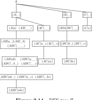
We now describe MineWithRounds which uses the partitioning defined before. Intuitively, it uses a loop which considers at each iteration the itemsets of the corresponding round. We use the following data structures : C is an array of sets of itemsets sets. C[i] is the set of candidates to be processed during round i and MFI is the set of MFI’s found so far. The right children of ABC are AC and BC (just do not consider its prefix). The right sibling of ABC is ABD (just replace the last item, here C, by its successor, here D). Note that if Round(I) = i and J is the right sibling of I then Round(J ) = i + 2. Intuitively, the algorithm proceeds as follows : If a candidate I ∈C[k] is found frequent, then its successor is a candidate for the next iteration k + 1. If I is infrequent then (i) its right children are potential candidates for the next iteration k + 1 and (ii) its sibling is a potential candidate for iteration k + 2. To explain the covering tests, suppose AC and BC are candidates tested during the same round. Suppose AC is frequent but not BC. Thus AC generates its parent ACD as a future candidate and BC generates both C (its right child) and BD (its sibling). Note that since C is covered by ACD, there is no need to consider it as a future candidate.
2.5. MineWithRounds Algorithm Algorithm 1: MineWithRounds 1 C[1] ← {I1}; 2 k ← 1; 3 while k ≤ 2n − 1 andC[k] 6= ∅ do 4 foreach I ∈C[k] do
5 // Loop executed in parallel
6 if support(I) ≥ σ then
7 Add I to MFI;
8 Remove the left child I0 of I from MFI; 9 Add the right parent I00 of I to C[k + 1]; 10 else
11 Add the right children of I to Children; 12 Add the right sibling of I to C[k + 2]; 13 foreach I ∈C[k + 1] do
14 // Loop executed in parallel
15 if I is covered by MFI then 16 Remove I fromC[k + 1]; 17 foreach I ∈ Children do
18 // Loop executed in parallel
19 if I is not covered by MFI then 20 Add I to C[k + 1];
21 k ← k + 1;
The reader should notice from the above algorithm description that the candidates are generated dynamically. Actually, at each stage, C[k] ⊆Rk. Rk is upward and downward pruned with respect to the previous computations.
In our implementation, the three Foreach loops in lines 4, 13 and 17 are executed in a parallel fashion. The first one essentially tests the support, the second checks the coverage of the sibling candidates that have been generated during iteration k − 1 and the last one tests the coverage of the children that have been generated during iteration k. It is worthwhile to note that there are barriers between these loops, i.e. the second loop cannot start before the first has finished.
The following theorem, which is our main result, compares the performance of the above algo-rithm with DF S.
Theorem 3. DFS and MineWithRounds perform exactly the same number of support compu-tations.
As a consequence, we can state the theoretical speed up with respect to the number of available processing units.
Corollary 1. Let T and Tp be respectively the computations times of DFS and MinWithRounds
when p processors are available. Then T
p ≤ Tp≤ T
p + (2n − 1)∆
Note that, since in general the number of candidates r is much larger than n, (2n − 1) ∗ ∆ can be neglected with regard to T /p. Hence, the speed up of MineWithRounds is almost perfect. The worst case is when ri mod p = 1, e.g. suppose p = 16 and ri= 33. Suppose that the 33rdtest takes 2sec and the others take 1sec. Then, the sequential algorithm requires 34sec. With p cores, the first 32 candidates are processed within 2sec while the last candidate requires 2sec by itself so a total of 4sec. Hence, the speed up is 34/4 = 8.5. Note that if we had 47 candidates and it is the 47th one which requires 2sec then the parallel total time is again 4sec and the speed up is this time equal to 48/4 = 12.
The following example illustrates the MFI’s computation with our algorithm.
Example 6. LetI = {A,B,C,D,E} and suppose that the maximal frequent itemsets are {ABDE,BC}. Figure 2.5 shows candidates generation. The arrows show candidates generation. For example, A is found frequent in round 1, therefore its parent AB is generated as a candidate. ABC is found infrequent during round 3, so its sibling ABD is generated together with its right children AC and BC. Candidates colored in red are those that are first generated then removed because they turn to be covered. For example, in round 4, AC is found infrequent so its right children C is generated as a candidate to be tested during round 5. But meanwhile, BC is found frequent. Hence, BC is added to the provisional set of MFI’s and its parent BCD is scheduled for round 5. Hence, when the execution of round 5 starts, we find C covered by BC. The same remark holds for the sibling AD of AC which is first generated for round 6 then removed because during round 5, ABD is found frequent. Note that in this small example just two iterations contain more than one candidate, namely iterations 4 and 5. Thus, with 2 processors just these rounds will benefit from parallelism. However, realistic data sets with much more items exhibit rounds with thousands of candidates.
A ABDE BCE CE CD BCD ABD AC BC ABC AB 1 2 3 4 5 6 7 8 9 C D E BD AD
Figure 2.5 – Rounds assignment and MineWithRounds computation
2.6
Data Distribution
In this section we show how to adapt our algorithm to the case when data is distributed. An obvious way to do so is to consider one distinguished node as the master and the others are slaves. The master is responsible of the candidates and the border management while the slaves compute the interestingness on their respective local data. At each iteration, (1) the master sends all candidates to all slaves, (2) each slave computes the local support of all candidates, (3) each slave sends its results to the master, (4) the master combines the partial results to find the global interesting candidates, (5) it updates the border and (6) it generates new candidates
In the MFI setting, the communication complexity is the total size of messages. Let ri be the the number of candidates processed during iteration i and p be the number of slaves. At each iteration i
2.7. MFI’s Mining Experiments
the master sends a message of size rito the slaves and each slave notifies the master with a message of length ri. Thus the total communication cost is 2pP2n−1i=1 ri. Of course, other implementations are possible, e.g., instead of computing the support of each candidate by every slave, we let the later to make this computation only if the already computed support is not sufficient to make the candidate frequent. This will reduce the overall computation time. As one can see, our proposal of candidates partitioning is orthogonal to the way data is distributed. In fact, it leads itself easily to Map-Reduce setting : it is essentially the same problem as computing the number of words occurrences.
2.7
MFI’s Mining Experiments
2.7.1 OpenMP
We implemented our algorithm using C++ and the STL library together with OpenMP [76] : a multi-shared programming API. OpenMP makes it very easy to exploit new multi-core architecture by just adding compilation directives. For example, the loop :
For (i=0; i<1000; i++) a[i]=f(i);
can be executed in parallel by adding just one line of code as follows
#pragma omp parallel for num_threads(4) schedule(dynamic) For (i=0; i<1000; i++)
a[i]=f(i);
The number of parallel threads that are launched in this case is fixed to 4. Moreover, OpenMP enables the user to choose how threads should be scheduled. In the example above, we have chosen a dynamic scheduling meaning that the fours parallel threads will execute respectively the instruc-tion a[i]=f[i], for i=1..4 then the first among them which terminates, will execute the same instruction by considering i=5, and so on. This type of scheduling is particularly interesting when the execution time of function f is variable depending on the i value. Our purpose here is not to explain the many facilities offered by OpenMP but rather to show how it is easy to parallelize source codes when using it.
We have checked the correctness of our implementation by comparing its results with other previous implementations (Mafia and PADS) as well as by considering the results reported in [31].
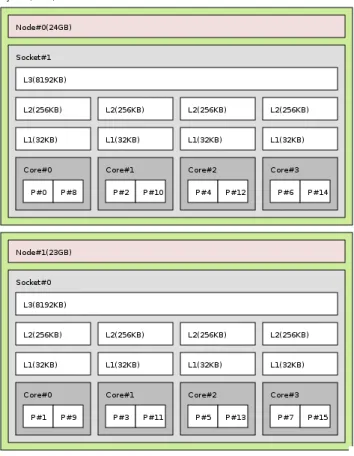
2.7.2 Machine
Our tests were conducted on a machine equipped with two quad-core Intel Xeon X5570 2.93GHz processors running under Redhat Linux enterprise release version 5.4. Thanks to their multi-threading ability, these processors can execute concurrently two threads per core. Therefore, we were able to launch up to 16 threads. Figure 2.6shows this internal structure. It shows for example that in node 1, core 0 contains two logical processing units p#0 and p#8 meaning that multi-threading is enabled.
2.7.3 Data sets.
We present the results we obtained with six well known datasets : Chess, Mushroom, T10I4D100K, T40I10D100K, Kosarak and Webdocs. Their respective characteristics are described in Table2.1.
Depending on the number of transactions, we categorized the samples into small, medium and large data sets. With each dataset, we varied the minimal support threshold σ and with every such value, we varied the number of parallel threads executed for every Foreach loop in the algorithm
Figure 2.6 – The internal structure of the machine used for our experiments.
Dataset # trans. # Items Avg. transact. Size length Chess 3196 75 37 Small Mushroom 8124 119 23 Small T10I4D100K 105 103 10 Medium T40I10D100K 105 103 40 Medium Kosarak ∼ 106 40348 8 Large Webdocs ∼ 1.7 ∗ 106 ∼ 5.3 ∗ 106 178 Large
2.7. MFI’s Mining Experiments
(the same number of threads for the three loops). This number varies from 1 to 16 as a power of 2. In order to gain load balancing, we used the dynamic scheduling of OpenMP.
2.7.4 Results Analysis
For each data set, we measured the time devoted to each of the three loops present in our algorithm (cf. Algorithm 1). The first loop essentially computes the support of a set of candidates while the two remaining loops make covering tests : One of them (line 17) tests the coverage of the candidates that have been generated as children of non frequent itemsets and the other (line 13) tests the candidates that have been generated as siblings. In our main theoretical result (Corollary
1), we claimed that when the time devoted to support computation is the dominating time, the speedup of our algorithm is almost perfect. The experiments not only confirm this result but also show that when this test is not very time consuming we still get interesting speed ups.
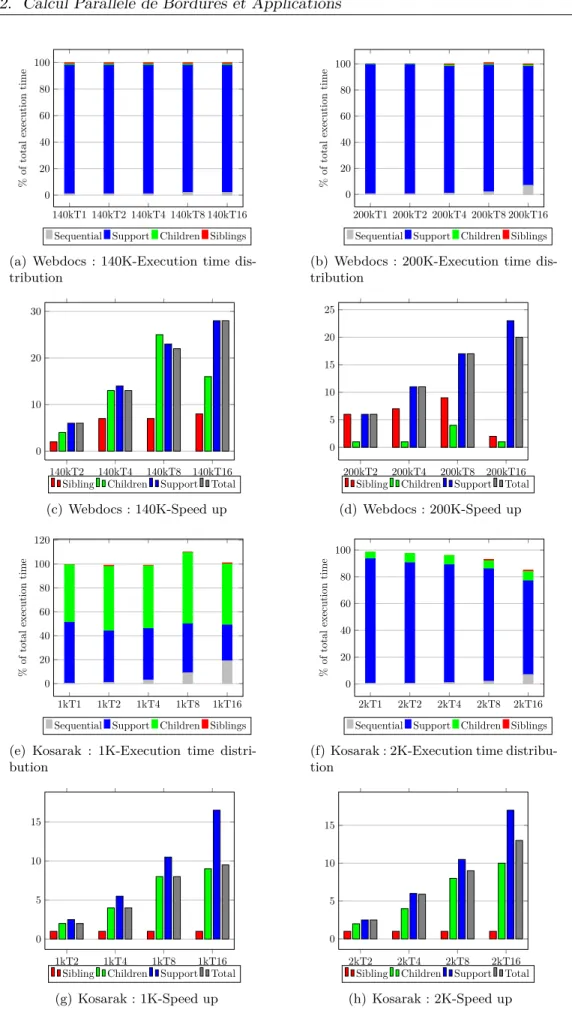
Figures 2.7, 2.8 and 2.9 show some of the obtained results. For each dataset, we consider two support thresholds and for each, there is one subfigure showing the proportion of time devoted to each of the three loops as well as the execution time of the sequential part of the algorithm. The second subfigure shows the speedup of each loop as well as the total speedup. The X_axis of each figure represents the minimal support value concatenated to the number of threads. For example, in subfigure2.7(a), 140K_T16 means that the minimal threshold is 140K and the number of threads is fixed to 16.
Large data
With Webdocs dataset, more than 90% of the time is consumed by the support computation (see Figures 2.7(a) and 2.7(b)). Hence, the speed up of the overall execution is almost equal to the support computation speed up. Note that Figure 2.7(c) shows a total speedup of 30 while the number of threads is just 16. Moreover, the number of physical processors is 8. This super-linear speed-up is explained by data locality. Indeed, when two threads access the same data, the system will first check the different levels of the cache before making an access to the memory. Recall from our partitioning technique that all the candidates with the same last item and the same total number of items are processed in parallel. For example, ACD, BCD and ABD. We use a prefix tree with a header to summarize the underlying data in the very same way as FP-trees do. Hence, for computing the support of ACD, we traverse the list of nodes associated to item D (the last one of the itemset). Each time we check whether the path from the root of the tree to the node contains ACD. It if is the case, the counter value of the node is added to the support of ACD. Note that the same list is traversed for BCD and ABD. Hence, if we have three different threads processing each of these three candidates, then we have good chances that one of them will bring the data (nodes of the prefix tree) from main memory to the different levels of the cache then to the register but the other threads could find it without accessing main memory making their computation much faster. To favor this optimization, we sorted the candidates wrt their last item. Moreover, we used an array structure to code the branches of the tree because dynamic node allocation does not guarantee space locality between successive nodes. We have been inspired by the data structures first proposed in [35] and further optimized in [61].
Even if the Kosarak data set is relatively large, we note that the proportion of time devoted to support computation is comparable to the time spent in covering tests when the minimal support σ is set to 1K (Figure2.7(e)). This is not the case when σ = 2k. We note however that the speedup for support computation is in both cases almost perfect(Figures 2.7(g)and 2.7(h)). Finally, we should notice that the average size of transactions is quite short (8 items). Thus, the maximal frequent
140kT1 140kT2 140kT4 140kT8 140kT16 0 20 40 60 80 100 % of total execution time
Sequential Support Children Siblings (a) Webdocs : 140K-Execution time dis-tribution 200kT1 200kT2 200kT4 200kT8 200kT16 0 20 40 60 80 100 % of total execution time
Sequential Support Children Siblings (b) Webdocs : 200K-Execution time dis-tribution 140kT2 140kT4 140kT8 140kT16 0 10 20 30
Sibling Children Support Total (c) Webdocs : 140K-Speed up 200kT2 200kT4 200kT8 200kT16 0 5 10 15 20 25
Sibling Children Support Total (d) Webdocs : 200K-Speed up 1kT1 1kT2 1kT4 1kT8 1kT16 0 20 40 60 80 100 120 % of total execution time
Sequential Support Children Siblings (e) Kosarak : 1K-Execution time distri-bution 2kT1 2kT2 2kT4 2kT8 2kT16 0 20 40 60 80 100 % of total execution time
Sequential Support Children Siblings (f) Kosarak : 2K-Execution time distribu-tion 1kT2 1kT4 1kT8 1kT16 0 5 10 15
Sibling Children Support Total (g) Kosarak : 1K-Speed up 2kT2 2kT4 2kT8 2kT16 0 5 10 15
Sibling Children Support Total (h) Kosarak : 2K-Speed up
2.7. MFI’s Mining Experiments
itemsets tend to be short as well. This reduces the impact of downward pruning exploited by DFS algorithms.
Medium Size Data
The dataset 40I10D100K of medium size is denser than T10I4D100K. Figures2.8(a)and2.8(b)
show that support computation time is important. Nevertheless, we do not reach the same speed ups as those with Webdocs. We note however that the total execution time is always divided by almost the number of threads.
The average length of the transactions in T10I4D100K data set is 10. Hence, maximal frequent itemsets are rapidly reached when DFS is used (note that in Kosarak, this average length is even lower). This makes support computation not very time consuming, even when the minimal support is set to 20 thanks to the summarization capacity of the FP-trees.
Small Data
Both these Chess and Mushroom data sets are small. Thus, it is not surprising to find that support computation is negligible w.r.t. candidates management (see Figure 2.9). With Chess, we note a bad speed up when σ = 800. These last two experiments tend to confirm that our proposed algorithm is rather tailored towards situations when support computation is the bottleneck of the execution time. Moreover, we note for Chess data set that the number of MFI’s grows rapidly even when the support threshold id high. For example, when σ = 800 (a minimal frequency of 25%) the number of MFI’s is more than 26000 (more than six times the number of original transactions). This makes coverage test harder than support computation. For Mushroom data set, we have to lower the support threshold to around 100 (frequency ∼ 1%) to make the number of MFI’s larger than the number of transactions. Nevertheless, it turns that coverage test takes much larger time than support test. The explanation for this is the "non uniform" behavior of the MFI’s length. For example, when σ is set to 10%, the longest MFI has 16 items while there is no MFI of length 13 or 14. This phenomenon has been noticed in [30].
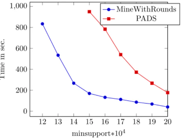
2.7.5 MineWithRounds vs PADS
As a final experiment, we present the execution time of PADS [101] which is, to our best knowledge, the most efficient implementation of a sequential MFI mining algorithm and compare it with that of MineWithRounds. PADS is not a pure DFS implementation in that it uses several heuristics to reduce computation time, e.g., each time a candidate is found frequent, all its right parents are evaluated and reordered w.r.t their increasing support. Hence, the ≺ order is dynamically and continuously modified. Figure 2.10 shows the execution times w.r.t. support thresholds. Both implementations have been executed on the same machine as before. The time needed to load the data and to construct the FP-trees is not taken into account. One should however notice that our execution time is measured when 16 threads are executed in parallel. It took about 2 minutes for both implementations to start the mining procedure. When the minimal support is less than or equal to 140000 PADS had a segmentation fault. To be complete, we should mention that our implementation is naive in that we used the C++ STL library which makes it very easy to program prototypes but if we want to fine tune the optimizations, as in PADS, one should program his/her own data structures2.
1kT1 1kT2 1kT4 1kT8 1kT16 0 20 40 60 80 100 % of total execution time
Sequential Support Children Siblings (a) T40 : 1K-Execution time distribution
2kT1 2kT2 2kT4 2kT8 2kT16 0 20 40 60 80 100 % of total execution time
Sequential Support Children Siblings (b) T40 : 2K-Execution time distribution
1kT2 1kT4 1kT8 1kT16 5
10
Sibling Children Support Total (c) T40 : 1K-Speed up 2kT2 2kT4 2kT8 2kT16 0 5 10 15
Sibling Children Support Total (d) T40 : 2K-Speed up 20T1 20T2 20T4 20T8 20T16 0 20 40 60 80 100 % of total execution time
Sequential Support Children Siblings (e) T10 : 20-Execution time distribution
100T1 100T2 100T4 100T8 100T16 0 20 40 60 80 100 % of total execution time
Sequential Support Children Siblings (f) T10 : 100-Execution time distribution
20T2 20T4 20T8 20T16 0
5 10 15
Sibling Children Support Total (g) T10 : 20-Speed up
100T2 100T4 100T8 100T16 0
5 10
Sibling Children Support Total (h) T10 : 100-Speed up
2.7. MFI’s Mining Experiments 100T1 100T2 100T4 100T8 100T16 0 20 40 60 80 100 % of total execution time
Sequential Support Children Siblings (a) Mushroom : 100-Execution time dis-tribution 200T1 200T2 200T4 200T8 200T16 0 20 40 60 80 100 % of total execution time
Sequential Support Children Siblings (b) Mushroom : 200-Execution time dis-tribution 100T2 100T4 100T8 100T16 2 4 6 8
Sibling Children Support Total (c) Mushroom : 100-Speed up 200T2 200T4 200T8 200T16 0 5 10 15
Sibling Children Support Total (d) Mushroom : 200-Speed up 800T1 800T2 800T4 800T8 800T16 0 20 40 60 80 100 % of total execution time
Sequential Support Children Siblings (e) Chess : 800-Execution time distribu-tion 1000T1 1000T2 1000T4 1000T8 1000T16 0 20 40 60 80 100 % of total execution time
Sequential Support Children Siblings (f) Chess : 1000-Execution time distribu-tion 800T2 800T4 800T8 800T16 0 5 10 15
Sibling Children Support Total (g) Chess : 800-Speed up
1000T2 1000T4 1000T8 1000T16 5
10
Sibling Children Support Total (h) Chess : 1000-Speed up
12 13 14 15 16 17 18 19 20 0 200 400 600 800 1,000 minsupport∗104 Time in sec. MineWithRounds PADS
Figure 2.10 – Execution times for PADS and MineWithRounds with Webdocs
2.8
Concluding Remarks on MFI’s Computation
We presented MineWithRounds, a parallel algorithm for computing maximal frequent item-sets. It mimics DFS in that it tests the support of exactly the same candidates. The theoretically proved speed up of our algorithm regarding the execution time devoted to supports computation is confirmed by the extensive experiments we conducted. With large datasets, this speed up is even better than what was expected thanks to cache management in modern machines.
With the generalization of multi-core CPU’s and their cache management, some proposals fine tuned the previous techniques so that data caching and pre-fetching become effective [35]. An efficient parallel algorithm for building the FP-trees has already been proposed by [61] but the mining process has been made data parallel not task parallel. Hence, no guarantee that the parallel process will be faster than the sequential version. With our present work, we make a step further in exploiting modern multi-core architectures. Our experiments show that without necessarily using very sophisticated optimization techniques, we are able to have execution times much better than state of the art implementations.
Parallelizing algorithms that extract other kinds of patterns e.g. sequences, trees or graphs is a natural extension of the present work, e.g. [96] use a canonical order for mining frequent graphs. By defining the parent/children/sibling relationships as analogously as we did for itemsets, then for extracting maximal frequent graphs, it suffices to use the fundamental idea behind our algorithm, i.e., start the evaluation of a subgraph as soon as all its left parents have been evaluated. We leave the development of this issue to future work.
Finally, we should mention that even if our implementation assumes a shared memory architec-ture, we showed in Section2.6 how it could be adapted to distributed data setting.
In the remaining part of this chapter, we shall turn our focus towards dependency mining.
2.9
Parallel Mining of Dependencies
The problem of extracting functional dependencies (FDs) from databases has a long history dating back to the 90’s. Still, efficient solutions taking into account both material evolution and the amount of data that are to be mined, are still needed. We propose a parallel algorithm which, upon small modifications, extracts (i) the minimal keys, (ii) the minimal exact FDs, (iii) the minimal approximate FDs and (iv) the Conditional functional dependencies (CFDs) holding in a relational table. Under some natural conditions, we prove a theoretical speed up of our solution with respect
2.10. Related Work w.r.t Mining Functional Dependencies
to a baseline algorithm which follows a depth first search strategy. Since mining most of these dependencies require a procedure for computing the number of distinct values (NDV) which is a space consuming operation, we show how sketching techniques for estimating the exact value of NDV can be used for reducing both memory consumption as well as communications overhead when considering distributed data while guaranteeing a certain quality of the result. Our solution is implemented and some experimental results are reported here showing the efficiency and scalability of our proposal.
2.10
Related Work w.r.t Mining Functional Dependencies
Several algorithms have been proposed to find the minimal set of FDs from a relation. These algorithms can be classified along three criteria : (i) the way they traverse the search space, i.e., breadth or depth first, (ii) pre-computation and (iii) incremental computation. TANE [52], FUN [75] and FD_Mine [99] use a levelwise strategy to explore the candidates lattice. They start by constructing a partition of the tuples for each attribute (two tuples belong to the same part with respect to some attribute A iff they share the same value A’s value) then they build new partitions from already constructed ones, i.e., they perform the partition product. If PX(T ) denotes the partition of relation T w.r.t. X then T satisfies X → A iff |PX(T )| = |PXA(T )| where |PX(T )|, resp. |PXA(T )|, denotes the number of parts there are inPX(T ), resp.PXA(T ). For example, suppose that PA(T ),PB(T ) and PC(T ) are computed. Then verifying whether AB → C consists in combining3 PA(T ) and PB(T ) to get PAB(T ) and then this result is combined with PC(T ) to get PABC(T ). The main difference between these algorithms resides in the pruning strategies they use. The three algorithms are incremental in the sense that the computation of the partitions at some level is made from the computed partitions of the previous one. Clearly, when data and/or the left hand side of the FDs are large, i.e., large number of candidates by level, the memory consumption becomes a sever bottleneck. In our experiments, this actually happened, i.e., the memory was saturated, even with moderate size data and not so excessive number of attributes (40). Dep-Miner [67] uses others concepts. It first computes the agree sets for each pair of tuples, that is the set of attributes for which they share the same values. Clearly, if ag(t1, t2) = X then T 6|= X → A for each A ∈A \ X.
After that, Dep-Miner computes maximal difference sets ( i.e., complements of agree sets) to build an hypergraph for each fixed target attribute and seeks their minimal transversals. Intuitively, this turns to compute minimal exact FDs from maximal incorrect FDs. The authors show that this method outperforms TANE. FastFD [94] uses the same technique as Dep-Miner but follows a depth first strategy when traversing the search space. The principal drawback of Dep-Miner and FastFDs is their pre-computation phase whose complexity is O(|T |2) which is prohibitive when T is large.
On another side, traversing the search space in breadth first reduces the pruning possibilities. Indeed, when a functional X → A is discovered, there is no need to test the supersets of X, we know a priori that they determine A, so they can be pruned. In the same time, if X → A doesn’t hold, then no need to test the subsets of X since they cannot determine A, so they are pruned. Breadth first traversal can utilize only one way pruning : upward or downward. One advantage however of BFS is that it can be naturally parallelized : all candidates of the same level are processed in parallel.
Our aim is to combine the advantages of each approach, i.e., use DFS in order to prune candidates both upward and downward, do not do any pre-computation and use parallelism. For this purpose, we adapt MineWithRounds algorithm. In fact, that algorithm can directly be used to mine the set of maximal FDs that "are not satisfied". The set of minimal FDs that are satisfied is actually the dual of the former set. It can be obtained by applying algorithms devoted to the