Sequential Pattern Generalization for Mining Multi-source Data

HAL Id: tel-03184696

https://hal.univ-lorraine.fr/tel-03184696

HAL is a multi-disciplinary open access archive for the deposit and dissemination of sci-entific research documents, whether they are pub-lished or not. The documents may come from teaching and research institutions in France or abroad, or from public or private research centers.

L’archive ouverte pluridisciplinaire HAL, est destinée au dépôt et à la diffusion de documents scientifiques de niveau recherche, publiés ou non, émanant des établissements d’enseignement et de recherche français ou étrangers, des laboratoires publics ou privés.

Sequential Pattern Generalization for Mining

Multi-source Data

Julie Bu Daher

To cite this version:

Julie Bu Daher. Sequential Pattern Generalization for Mining Multi-source Data. Computer Science [cs]. Université de Lorraine, 2020. English. �NNT : 2020LORR0204�. �tel-03184696�

AVERTISSEMENT

Ce document est le fruit d'un long travail approuvé par le jury de

soutenance et mis à disposition de l'ensemble de la

communauté universitaire élargie.

Il est soumis à la propriété intellectuelle de l'auteur. Ceci

implique une obligation de citation et de référencement lors de

l’utilisation de ce document.

D'autre part, toute contrefaçon, plagiat, reproduction illicite

encourt une poursuite pénale.

Contact : ddoc-theses-contact@univ-lorraine.fr

LIENS

Code de la Propriété Intellectuelle. articles L 122. 4

Code de la Propriété Intellectuelle. articles L 335.2- L 335.10

http://www.cfcopies.com/V2/leg/leg_droi.php

´

Ecole doctorale IAEM Lorraine

Sequential Pattern Generalization for

Mining Multi-source Data

TH`

ESE

pr´esent´ee et soutenue publiquement le 10 D´ecembre 2020

pour l’obtention du

Doctorat de l’Universit´

e de Lorraine

par

Julie BU DAHER

Composition du jury

Pr´esidente : Isabelle DEBLED-RENESSON Professeur, Universit´e de Lorraine

Rapporteurs : Marie-H´el`ene ABEL Professeur, Universit´e Technologique de Compi`egne Nicolas LACHICHE Maˆıtre de conf´erences, Universit´e de Strasbourg Directrice : Armelle BRUN Maˆıtre de conf´erences, Universit´e de Lorraine

Sommaire

Introduction 1

1 General context . . . 1

2 Problem statement . . . 3

3 Approach and contributions . . . 4

4 A link with the educational domain . . . 5

5 Plan of the thesis . . . 5

1 Related Work 1.1 Sequential pattern mining (SPM) . . . 7

1.1.1 SPM algorithms using horizontal representation . . . 11

1.1.2 SPM algorithms using vertical representation . . . 13

1.2 Multi-* data. . . 15

1.2.1 Multi-source data . . . 15

1.2.2 Relational data . . . 17

1.2.3 Multi-dimensional data . . . 17

1.3 Mining multi-* data . . . 19

1.3.1 Multi-source pattern mining . . . 19

1.3.2 Relational pattern mining . . . 22

1.3.3 Multi-dimensional pattern mining. . . 23

1.3.4 Multi-dimensional pattern mining using star schema . . . 32

1.3.5 Contextual sequential pattern mining. . . 34

1.4 Conclusion. . . 37

2 G_SPM Algorithm for Mining Frequent General Patterns 2.1 Data sources description in multi-* dataset . . . 40

2.1.1 Sequential data source . . . 40

2.2 Proposition for a structure of relations between data sources . . . 41

2.2.1 Contextual relation . . . 42

2.2.2 Complementary relation . . . 44

2.3 Proposition for managing relations . . . 44

2.3.1 Managing contextual relation . . . 45

2.3.2 Naive approaches for managing complementary relation . . . 45

2.4 Preliminary definitions . . . 47

2.4.1 Infrequent patterns . . . 47

2.4.2 Promising patterns . . . 48

2.4.3 Sequence and item similarity . . . 48

2.4.4 Sequence generalization . . . 50

2.5 G_SPM algorithm for mining general sequential patterns . . . 53

2.5.1 Mining frequent sequential patterns. . . 53

2.5.2 Determining similar patterns among promising patterns . . . 55

2.5.3 Determining similar items among similar patterns. . . 55

2.5.4 Generalization of similar patterns having similar items . . . 56

3 Experiments and Results 3.1 Description of the application dataset . . . 61

3.1.1 The dataset extracted from this corpus. . . 62

3.2 Evaluation measures . . . 63

3.3 Experimental evaluations of the naive approach . . . 64

3.4 Experimental evaluation of G_SPM algorithm . . . 65

3.4.1 Impact of minsupProm. . . 65

3.4.2 Impact of the minimum pattern similarity . . . 69

3.4.3 Impact of the minimum item similarity. . . 71

3.5 Conclusions . . . 72

4 Conclusion and Future Work 4.1 Conclusion. . . 75

4.2 Future work . . . 76

4.2.1 Future experiments . . . 76

4.2.2 Future research work . . . 77

Table des figures

1.1 Relational database . . . 18

1.2 A hierarchy of food products [18] . . . 19

1.3 Blocks defined on Table 1.10 over dimensions CG and C [46] . . . 28

1.4 A taxonomy of food categories [22] . . . 29

1.5 Hierarchy of dimension "Product" . . . 30

1.6 Hierarchy of dimension "location" . . . 30

1.7 Taxonomies for hospitals and diagnoses. . . 31

1.8 Block partitioning of the database according to the reference dimension (Patient) 32 1.9 Star schema structure of movies database [55] . . . 33

1.10 Hierarchy of dimension "City". . . 35

1.11 Hierarchy of dimension "Age Category" . . . 35

1.12 Context hierarchy of context dimensions "City" and "Age Group" of Table 1.8 . 35 2.1 A 3-source dataset with contextual and complementary relations . . . 43

Introduction

1

General context

If there is one thing in the world that is too big to ignore, it is the creation of enormous amounts of data across years. Every single day, over 2.5 quintillion bytes of data are being created. Data has become important and indispensable in our everyday life, where 90% of the world’s data has been created in the last two years1, and it is estimated that 1.7 mega bytes of data will be created every second for each human being on the planet by the year 20202. This explosive growth of produced data volume is a result of the computerization of our society and the fast development of powerful data collection and storage tools [23], and this is what makes our age the data and information age and thus, generally, the digital age. Digital data exists in all research and business domains ; examples of these domains are e-commerce, healthcare, banking, education, etc.

In addition, these data can be easily collected where they can be of great volumes, and the variety of these collected data is as important as their volumes. Indeed, data can be collected from multiple data sources where each data source can provide one or more various kinds of data. Therefore, these various multi-source data form heterogeneous multi-source datasets. For example, in the domain of e-commerce, the data about customers can include their descriptive data, their past purchases, their feedbacks about their purchases, etc.

When these data are collected, they become available for analytics. Data analytics is the science of examining raw data with the aim to draw conclusions from the information they contain3. Data analytics technologies and techniques have become more and more important across time and are now widely used. Researchers and scientists are aware of the importance of data analytics in order to obtain valuable information that helps in proving or disproving their scientific hypothesis. Data analytics is also important in commercial industries as it helps organi-zations in taking informed and business decisions ; for example, it can help business increase their revenues or improve their efficiency and performance. In this frame, understanding customers’ data is an indispensable first step in order to take decisions such as predicting future purchases of customers or recommending them purchases upon their needs and preferences. There exist different approaches to analyze and understand the data and draw conclusions from the infor-mation they contain. Choosing a suitable approach depends on the nature of data as well as on the purposes of these analyses and the desired information to be obtained.

One of these approaches is Knowledge Discovery in Databases (KDD) that has been first de-fined by Fayyad et al., [13] as the non-trivial process of identifying valid, novel, potentially useful and ultimately understandable patterns in data. KDD can be generally divided into three main

1. www.sciencedaily.com retrieved on December 10th _{, 2019}

2. https ://www.domo.com retrieved on December 10th_{, 2019}

steps : pre-processing, data mining and post-processing [23]. The pre-processing step filters and prepares data by removing irrelevant, unreliable, redundant or noisy data. The post-processing ensures making the results understandable and then evaluates these results according to the requirements and the purposes. The data mining step aims at extracting knowledge from large datasets. These large datasets can be found in various kinds of databases such as relational data-bases, transactional datadata-bases, data warehouses and other data repositories. Data mining is the most challenging step of KDD process and is essential for many analytics tasks. It is the main focus of our research study. Data mining is defined as the process of identifying valid, novel, potentially useful, and ultimately understandable patterns in data [13].

There are three main techniques in data mining : classification [11], clustering [30] and pattern mining [2, 23]. Classification is defined as the process of finding a model (or function) that describes and distinguishes data classes or concepts. The model is derived from the analysis of a set of class labeled data. The model is used to predict the class label of objects for which the class label is unknown [23].

Unlike classification, which analyzes class-labeled objects, clustering analyzes objects without consulting class labels. Clustering is defined as the creation of groups or clusters of similar objects that are dissimilar to those of other clusters. Clustering methods are particularly useful for exploring the interrelationships among the data objects from the dataset and are one way of assigning class labels to the data objects when no such information is available or known [20].

Frequent pattern mining aims at finding patterns that are relevant and frequent in the data. Frequent pattern mining, with its different techniques, has grown to become an important topic across time where various works were proposed in these domains. The pattern mining process as well as the frequent patterns generated from this process are interpretable which would help in taking interpretable decisions such as recommendations. For example, pattern mining can be used in the healthcare domain where data scientists or researchers aim to analyze and understand the data about patients’ symptoms, the diagnoses made by doctors based on these symptoms and the treatments prescribed by doctors to patients according to these diagnoses. Based on these data, they can extract frequent patterns where a frequent pattern contains certain symptoms, their diagnosis and their treatment. These patterns thus allow them to recommend relevant treatments for patients according to their symptoms.

Sequential pattern mining is one of the various types of frequent pattern mining. It is concer-ned in finding frequent patterns in datasets whose items are organized in the form of sequences where a sequence is an ordered list of items or itemsets. Sequential pattern mining is a topic of high interest as sequential data exists in many application domains such as e-learning where sequential data can represent the sequences of pedagogical resources (exams, quizzes, exercises, etc.) that the students consult on their virtual learning environments (VLE) ; an example of such kind of student sequence is as follows : Student-143 : < R₃R8R13R27R29 > where Student-143

represents the id of a student and Rn represents the id of a pedagogical resource. The sequence

means that the student has consulted the resources R₃, then R₈, then R₁₃, then R₂₇ and finally R29. A frequent pattern extracted from this sequence can be : P : < R13R27R29>. By extracting

frequent patterns of pedagogical resources of students, we can form rules to recommend resources to the students based on their past activity. For example, based on the frequent pattern p, if a student has already consulted the resources R₁₃ and R₂₇, then we can recommend him/her the resource R29.

As previously mentioned, a dataset can contain several types of data which can come from multiple data sources. Data can be sequential and can for example represent data sequences of transactions performed by the users on their system ; an example of this data is the product purchases performed by customers from an e-commerce website. Data can also represent

des-2. Problem statement criptive data about users ; an example of this data is the demographic data of users such as their age, gender and address. Data can also represent descriptive data about items. Considering the example of customer purchases from an e-commerce website, the descriptive data about the products purchases by customers could be product name, brand and expiry date. These various data sources, put together, form a complex and a heterogeneous data set. Despite its complexity and heterogeneity, such a dataset is rich, and we assume that, if accurately mined, it allows providing rich information which makes the mining of such a dataset a challenge.

2

Problem statement

The general objective of this PhD thesis is the mining of frequent patterns from multi-source datasets. The data to be mined can be complex, heterogeneous and can contain various kinds of data. Data can be sequential (or temporal) or descriptive and can occur in different forms such as numerical, categorical, textual or graphical forms. Our applicative objective is analyzing and understanding the behavior of users. The data used to perform this analysis can represent several points of view of this behaviour, can come from multiple data sources and can be of various kinds. By understanding this data, we aim to predict the behaviour of users and provide them with recommendations in a personalized manner. For this sake, we focus on mining sequential patterns from the multi-source data in order to extract frequent sequential patterns out of users’ behavioural data.

When the data is multi-source, if we limit the mining process to the mining of only one source, naturally the behavioral one, we consider that the results can be restricting for two main reasons. First, the patterns represent the data that are mined ; therefore, when only one data source among the multiple data sources is mined, the patterns will only contain information from this single source thus representing a unique point of view. Obviously, when additional sources are available, the mined patterns may contain information from these sources and will probably be richer. For example, when we uniquely manage the sequential data source, we would only understand the digital behaviour of users, and thus we would provide recommendations to the users based only on this information. However, this information may not be sufficient to provide reliable and well personalized recommendations. Therefore, adding descriptive information about the users and/or the items of the data sequences may result in a better understanding of the digital behaviour of users and thus in richer and more specific recommendations.

The second reason is that even when the amount of data is big, in certain cases we may face a problem of lack of data either caused by the data sparsity, by the variability of human behavior or by the similarities among the data which will be further explained in the following chapters. These similarities can be on the level of items of the sequences where we can find certain items that are similar to others, and they can be on the level of patterns where certain patterns are similar to others. Therefore, there could be patterns which could not be detected as being frequent due to the similarities among them. This problem leads to a decrease in the number of the generated sequential patterns and thus a lower data coverage. In this case, the extracted information would be limited. Therefore, when several data sources are available, it is important to manage these sources in order to limit the problem of similarity and generate frequent patterns containing information from these different sources.

Various techniques have been proposed to mine multi-source data [45, 60, 67, 12, 43, 69]. These techniques can be divided into two main approaches. The first approach mines different data sources in a separate manner. A separate mining process is performed for each data source, and the information extracted from all the mining processes is then combined to obtain global

information which contains various kinds of information coming from different data sources. This approach allows obtaining valuable information. However, the major limitation of this approach lies in the fact that some data sources may provide useful information only if they are mined with other data sources ; thus, mining this source separately will result in useless or insufficient information. In addition, this approach leads to a loss of information when there is a problem of similarity in a data source.

This allows us to understand that different data sources are interrelated, that is having different kinds of relations among each other where certain data sources provide data to other sources. This approach would lead to the loss of important information due to the loss of the relations existing between different data sources. The second approach manages multi-source data by integrating all data sources in the dataset together and mining them in a single mining process. This approach maintains the relations between the data sources, which avoids data loss and allows generating rich information. However this approach results in a complex form of data that represent the input of the mining process which also has a high complexity, especially when there is a large number of data sources where each one provides different kinds of data.

Based on the limitations of both approaches, the main challenge in our work lies in how to mine a complex dataset formed of multiple heterogeneous and interrelated data sources by managing the relations existing among different sources and taking into consideration the algorithm complexity in order to extract rich and useful informa-tion in the form of sequential patterns containing various kinds of informainforma-tion and to compensate the loss of information caused by the problem of data similarity.

3

Approach and contributions

We propose an approach that manages multi-source data in a single process. In this frame, we propose to limit the complexity by using a strategy of selective mining where additional sources are mined only when needed during the process. This approach is designed to be generic as it is not restricted to data of a specific domain or structure.

As mentioned in section2, we notice that there may be different relations among data sources. In this context, we distinguish between two kinds of relations among the sources. The first kind of relations exists between the sequential data source and the descriptive data source of users where the latter provides specific information to each user thus allowing to obtain more precise frequent sequential patterns than the ones generated from a traditional mining of sequential data.

On the other hand, the second kind of relations exists between the sequential data source and the descriptive data source of items where the latter provides additional data about each item in the data sequences. A data sequence, representing a sequence of item ids, is thus pro-vided by additional descriptive attributes to each item. These attributes represent more general information than item ids, and thus they provide more generality to the sequential data source. In our proposed approach, we manage the two kinds of relations while mainly focusing on the second kind by taking advantage of the descriptive data source of items in order to generate general sequential patterns. In order to overcome the problem of data similarity and thus generate more frequent patterns, we define two similarity measures in order to compare different patterns and the items that they contain : pattern similarity and item similarity. Then, we form general patterns from the similar patterns containing similar items where a general pattern is a pattern that contains more general information than traditional frequent patterns. Finally, we propose a novel method of support calculation of this new kind of patterns in order to detect frequent

4. A link with the educational domain general patterns.

Hence, our approach solves the problem of data similarity and low data coverage by generating more frequent patterns ; in addition, the frequent general patterns formed are rich as they contain various kinds of information.

4

A link with the educational domain

The use of technology to better understand how learning occurs has received considerable attention in recent years [19]. Digital educational data, whether concerning learning or teaching processes, is collected from VLE’s and information systems of educational institutions, and they are now available for analytics for different purposes.

"Learning analytics" (LA) is best defined as "the measurement, collection, analysis and re-porting of data about learners and their contexts, for purposes of understanding and optimizing learning and the environments in which it occurs” [36]. It aims at improving the learning process by giving learners the ability to evaluate their academic progress and enhance their achievements and motivation.

Our work is funded by PIA2 e-FRAN METAL project4. The aim of the project is to design, develop and evaluate a set of individualized monitoring tools for school students or teachers (Learning Analytics and e-learning), and innovative technologies for personalized learning of written languages (French grammar) and orally (pronunciation of modern languages). It thus contributes to the improvement of the quality of learning and the development of language proficiency by students. Our work is specifically dedicated to school students where the objective is to contribute to the improvement of their learning process.

In the domain of education, digital data are collected from multiple data sources which could provide various kinds of data forming a multi-source and heterogeneous dataset. Hence, our proposed approach can be applied on this dataset in the purpose of providing students with personalized recommendations of pedagogical resources in order to help them improve their academic performance through learning analytics.

The proposed model has been designed for educational purposes, while being generic. Due to a problem of data availability in the project, we have not yet been able to evaluate our model on educational data. For this reason, we evaluate the model using a music dataset which has an adequate structure to our proposed model. Once we are able to obtain the educational dataset of the project, we will evaluate our model using this educational dataset as well.

5

Plan of the thesis

The rest of the thesis is organized as follows. Chapter 1 presents the state of the art in our research domain. We start by presenting the state of the art in the domain of sequential pattern mining. Then, we discuss the multi-* data that represents multi-source, multi-dimensional and relational data. After discussing the multi-* data, we present the state of the art in the domain of multi-* pattern mining and contextual pattern mining.

Chapter 2presents our scientific contributions and the proposed algorithm. In this chapter, we first present a description of the various data sources in a multi-* dataset. We then discuss our proposition for a structure of relations among data sources. After that, we present G_SPM algo-rithm for mining frequent general patterns in multi-* data. Chapter 3 presents the experimental

results and evaluations of our proposed algorithm. We start by a description of the application dataset, then we discuss the evaluation measures that we determined for evaluating G_SPM. We then discuss the experimental evaluations of G_SPM compared to naive approaches, and we conclude the chapter with discussions and conclusions of the conducted experiments. Finally, we conclude the thesis manuscript and discuss the future perspectives in chapter 4.

1

Related Work

Contents

1.1 Sequential pattern mining (SPM). . . 7

1.1.1 SPM algorithms using horizontal representation. . . 11

1.1.2 SPM algorithms using vertical representation . . . 13

1.2 Multi-* data . . . 15

1.2.1 Multi-source data. . . 15

1.2.2 Relational data . . . 17

1.2.3 Multi-dimensional data . . . 17

1.3 Mining multi-* data . . . 19

1.3.1 Multi-source pattern mining. . . 19

1.3.2 Relational pattern mining . . . 22

1.3.3 Multi-dimensional pattern mining . . . 23

1.3.4 Multi-dimensional pattern mining using star schema . . . 32

1.3.5 Contextual sequential pattern mining . . . 34

1.4 Conclusion . . . 37

Data has been generated and collected enormously in all domains across decades. Nowadays, data is generated not only by enterprises in the industry sector, but also by individuals on a daily basis. There is an increasing number of techniques that facilitate the collection and storage of the digital data. In this context, many frequent pattern mining approaches were proposed in the literature to analyze and understand the data and then extract useful knowledge that serves business or research purposes. In this chapter, we present the literature review in the domain of sequential pattern mining, that is the approach that we have identified as the most adequate to the kinds of data that we have as well as to the scientific problems that we address. Then, we present the various kinds of data. After that, we present a literature review of the most interesting research works proposed for mining these various kinds of data. Finally, we present a global conclusion of the related work.

1.1

Sequential pattern mining (SPM)

Agrawal and Srikant [3] were the first to address the problem of sequential pattern mining, and they defined sequential pattern mining as follows :

"Given a database of sequences, where each sequence consists of a list of transactions ordered by transaction time and each transaction is a set of items, sequential pattern mining is to discover

all sequential patterns with a user-specified minimum support, where the support of a pattern is the number of data-sequences that contain the pattern."

In this work, they stress on the importance of adopting property 1.1.1 for mining frequent sequences in an efficient manner, which states that the support decreases with the sequence exten-sion. Therefore, if a sequence is infrequent, then this directly implies that all its supersequences are infrequent too and thus there is no need to generate these candidates.

Sequential pattern mining has grown to be a topic of high interest and has become essential to many application domains like customer purchases, medical treatments, bioinformatics, etc. For example, in the domain of customer purchase analysis, customer shopping sequences represent the purchase behaviour of the customers as follows : a customer first buys a Sony smartphone, then a Sharp television then a Sony digital camera.

All sequential pattern mining algorithms have a sequential database and a user-defined mini-mum support threshold (minsup), and generate all frequent sequential patterns as the algorithm output.

In what follows, we present the definitions that allow the understanding of the sequential pattern mining.

Definition 1.1.1. (Sequence)

Let us consider that {I = I1, I2..., In} is a set of n items, si is an itemset that contains an

unordered set of items from I. siis also called an element or an event. A sequence s is an ordered

list of itemsets and is denoted by s =< s₁, s2..., sm >.

Definition 1.1.2. (Length of a sequence)

The length of a sequence s, denoted by l(s) is determined as the total number of instances of items in this sequence. A sequence with length l is called an l-sequence.

Definition 1.1.3. (Subsequence and supersequence of a sequence)

A sequence s =< s1, ..., sk > is a subsequence of the sequence t =< t1, ..., th >, denoted as

s ⊆ t, if there exist integers 1 ≤ i1 < i2 < i3... < ij such that s1 ⊆ ti1, s2 ⊆ ti2 ..., sk ⊆ tij. In

this case and for the same conditions, t is a supersequence of s, denoted as t ⊇ s. Definition 1.1.4. (Sequential database)

A sequential database S_D is a set of tuples, < sid, s_id > where sid is a sequence and sid is

the identifier of this sequence.

Definition 1.1.5. (Support of a sequence)

The support of a sequence s is defined as the number of sequences in the database containing s. Let us consider the sequential database SD and the sequence s =< s1...sk>, the support of s,

denoted as support_(S

D)(s) is calculated as follows :

support(SD)(s) = |{(< sid, sid>) ∈ SD; s ⊆ sid}| (1.1)

Definition 1.1.6. (Frequent sequence)

Let us consider a minimum support threshold, denoted as minsup. A sequence s is frequent in a sequence database S_D if support_(S

D)(s) > minsup. In other words, s is frequent only if it

occurs at least minsup times in SD. A frequent sequence is called a sequential pattern.

Property 1.1.1. (Anti-monotonicity property)

Given a sequential database SD over I and two sequences s and s0.

s ⊆ s0 =⇒ support(SD)(s) ≥ support(SD)(s

1.1. Sequential pattern mining (SPM) Example 1.1.1. (Sequential pattern mining)

Let us consider in Table 1.1 an example presented in [21] of a sequential database S_D that represents customer purchases . The set of items in S_D is {a,b,c,d,e,f,g}, and the minsup is set to 3. The sequence s4 : < {e}{g}{af }{c}{b}{c} > contains 6 itemsets : {e}, {g}, {af }, {c}, {b},

and {c}. This sequence means that this customer purchased e then g ; then, he/she purchased a and f at the same time ; after that, he/she purchased c then b then c. There are 7 instances of items in this sequence ; therefore, it is a 7-sequence. The item c occurs in 2 itemsets of this sequence : the fourth and the sixth itemsets ; however, the sequence contributes only one to the support of the item c. The sequence s0₄ : < {b}{c} > is considered as a subsequence of s₄ as the itemsets of the former are subsets of the itemsets in s4 respecting the order of the itemsets. The

support of the sequence s0₄ in S_D is 3 as it appears in 3 sequences of the database (sequence 1, 3 and 4). Sequence s0₄ is considered as a frequent sequential pattern as support_(S

D)(s) > minsup.

Table1.2 displays all sequential patterns in SD with their support values.

sid Sequence

1 <{a}{abc}{ac}{d}{cf}> 2 <{ad}{c}{bc}{ae}> 3 <{ef}{ab}{df}{c}{b}> 4 <{e}{g}{af}{c}{b}{c}> Table 1.1 – Sequence database SD

Sequence Support <{a}> 4 <{b}> 4 <{c}> 4 <{e}> 3 <{f}> 3 <{a}{b}> 4 <{a}{c}> 4 Sequence Support <{b}{c}> 3 <{c}{b}> 3 <{c}{c}> 3 <{d}{c}> 3 <{a}{c}{b}> 3 <{a}{c}{c}> 3

Table 1.2 – Frequent sequential patterns with minsup = 3 Definition 1.1.7. (Sequence prefix)

Let us consider the sequences s =< s₁, s2..., sk > and t =< t1, t2..., tl > where si and ti are

frequent itemsets in s and t respectively and l _{6 k. t is a prefix sequence of s if ti} = si for

(i 6 l − 1) and tl ⊆ sl as long as the remaining items of sl that is (sl− tl) are considered after

the items of t_l according to the alphabetical order. Definition 1.1.8. (Sequence suffix)

Let us consider the sequences s and t previously defined in definition1.1.7 where t is a prefix of s. Sequence u =< u₁, u2..., um > is called the suffix of s with respect to prefix t if and only if

∃ i 6 k, u = (si− tl) and ∀ 1 < j 6 m, (uj = si+j−1).

Example 1.1.2. (Sequence prefix and suffix)

Let us consider a sequence s =< {ef }{ab}{df }{c}{b} > which is the third sequence in the sequential database of our running example that is represented in Table 1.1. The sequences : <

{e} >, < {ef } >, < {ef }{a} >, < {ef }{ab} > are prefixes of the sequence s. < {ab}{df }{c}{b} > is a suffix of the sequence s with respect to prefix < {ef } >, and < {_b}{df }{c}{b} > is a suffix of s with respect to the prefix < {ef }{a} >.

Various approaches have been proposed across years to manage the problem of sequential pattern mining of sequential databases. The differences among all the proposed algorithms are in the choice of search space navigation, the database representation as well as the different data structures used for representing the input database which affects the mining process.

Sequential pattern mining algorithms traverse the search space to generate their candidate sequential patterns using either first or depth-first search enumeration. The breadth-first search enumeration, also named level-wise enumeration, explores all items that are found at one level and then moves down to explore the items of the next level. First, it explores all the singletons (1-sequential patterns) and generates frequent ones ; then, it extends the frequent singletons to generate all frequent 2-sequential patterns, then it extends frequent 2-sequential patterns to generate all frequent 3-sequential patterns, and so on until the last level where all frequent sequences are generated. The representative algorithms of the breadth-first search enumeration are the Apriori-based ones such as GSP algorithm [56].

The depth-first enumeration extends a sequential pattern until the minimum support thre-shold is not satisfied instead of exploring all l-pattern candidates before going forward to l + 1-pattern candidates. It starts from the singleton sequences and extends it to generate frequent 2-sequential patterns, 3-sequential patterns, 4-sequential patterns and so on until there are no more possible extensions. Then the algorithm goes backward to find more patterns from other sequences. Examples of algorithms which adopt the depth-first enumeration are PrefixSpan [41] and SPADE [64] algorithms.

Sequential pattern mining algorithms are classified into two categories, apriori-based algo-rithms and pattern growth-based algoalgo-rithms. Apriori-based sequential pattern mining algoalgo-rithms are based on AprioriAll algorithm [3], the first sequential pattern mining algorithm which is ins-pired by Apriori algorithm [4] for frequent itemset mining. Apriori-based algorithms explore the database search space using breadth-first search enumeration in order to generate frequent candidate patterns, and it scans the database repeatedly to calculate their support.

Pattern growth-based algorithms are based on FP-growth algorithm [26] that has been pro-posed as an improvement to Apriori algorithm [4] and thus generally to Apriori-based algorithms. These algorithms explore the database using depth-first enumeration. Pattern growth-based al-gorithms do not require generation where they scan the database to explore (k + 1)-candidate patterns from (k)-candidate patterns.

There are two kinds of representations of the sequential databases, the horizontal and the vertical database representations.

A horizontal database representation consists of a set of sequences where each sequence has an identifier followed by an ordered set of itemsets that occur in this sequence.

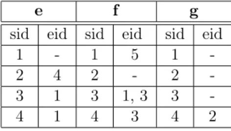
A vertical database representation consists of a set of items where each item is associated with each sequence identifier (sid) and itemset/event identifiers (eid) where this item occurs, also indicating a timestamp of the item in sid. This information is referred to as the id-list of the item.

A horizontal database can be transformed into a vertical database in one database scan, and we can also retrieve a horizontal database from a vertical one. Table 1.1 is an example of a horizontal database representation showing the sequence of items and itemsets represented by their sequence identifiers. Table1.3 and 1.4displays the vertical representation of Table1.1 for the items showing each item along with the sequences and the itemsets/events in each sequence

1.1. Sequential pattern mining (SPM) where this item occurs.

Example 1.1.3. (id-list in a vertical database representation)

Let us consider the item d in Table1.3. The id-list of the item d can be represented as follows : < d : (1, 4), (2, 1), (3, 3) >. Item d has appeared in the fourth itemset of the first sequence, in the first itemset of the second sequence and in the third itemset of the third sequence of the sequential database.

a b c d

sid eid sid eid sid eid sid eid

1 1, 2, 3 1 2 1 2, 3, 5 1 4

2 1, 4 2 3 2 2, 3 2 1

3 2 3 2, 5 3 4 3 3

4 3 4 5 4 4, 6 4

-Table 1.3 – Vertical representation of the database displayed in -Table1.1(1)

e f g

sid eid sid eid sid eid

1 - 1 5 1

-2 4 2 - 2

-3 1 3 1, 3 3

-4 1 4 3 4 2

Table 1.4 – Vertical representation of the database displayed in Table1.1(2)

In the following subsections, we present one sequential pattern mining algorithm from each of the two kinds of database representation.

1.1.1 SPM algorithms using horizontal representation

Sequential pattern mining algorithms using a horizontal database representation are classi-fied into apriori-based and pattern growth-based algorithms. In this subsection, we present a sequential pattern mining algorithm from each category.

Apriori-based algorithms

Some apriori based sequential pattern mining algorithms using horizontal database represen-tation are GSP [56], PSP [37] and MFS [68]. From this category, we present GSP , a well-known algorithm as it is one of the first sequential pattern mining algorithms.

GSP algorithm In 1996, Srikant and Agrawal proposed GSP algorithm (Generalized Se-quential Pattern mining algorithm) [56] to mine seSe-quential patterns. It is an improved version of the first sequential pattern mining algorithm, AprioriAll [3], that is proposed by the same authors.

As in Apriori algorithm [4], GSP algorithm adopts a multiple-pass, candidate-generation-and-test approach according to property1.1.1. The algorithm works as follows.

It makes multiple scans over the database. The first scan determines the support of each item. Hence, after the first database scan, the algorithm knows which items are frequent. Each frequent item found is considered as a 1-sequential pattern.

Each subsequent pass starts with a "seed set" that consists of the frequent patterns found in the previous pass. This seed set is used to generate new potentially frequent patterns that are named candidate patterns where each one contains one more item than a seed sequence. The support for these candidate patterns is found during a database scan. At the end of the pass, the algorithm determines which of the candidate patterns are actually frequent. These frequent candidate patterns become the seed for the next step. The algorithm stops when no more frequent patterns are generated.

At the (l+1)-level pass, the candidate frequent pattern generation is done by a joining process of two l-patterns as follows. A sequence s₁ joins with s₂ if by dropping the first item of s₁ and the last item of s2, the same subsequences are obtained. Therefore, s1 is extended with the last

item or itemset of s2 to obtain the new k + 1-candidate pattern

GSP is an important and well-known algorithm in the domain of sequential pattern mining ; however, it has some limitations. GSP performs multiple scans of the sequential database in order to calculate the supports of candidate frequent patterns to evaluate if they are frequent. The repetitive scans of the database lead to a high cost especially for huge databases. In addition, due the to the joining process to obtain (l+1)-candidate frequent pattern, two sequences can satisfy the conditions of join and thus would be extended to generate an (l+1)-candidate frequent pattern ; however, this may be a non-existing or infrequent sequence in the database. This process thus leads to a useless increase of the time complexity of the algorithm.

Pattern growth-based algorithms

A main advantage of pattern growth-based algorithms is the generation of frequent sequential patterns without candidate generation : only patterns that actually exist in the database are explored. However, the repetitive scans of the database is a process of high cost ; therefore, a new concept of database projection [40, 41, 27] has been proposed From this category, we present PrefixSpan algorithm. Among pattern growth-based approaches, PrefixSpan has been widely used in the literature in various research works in the domain of sequential pattern mining [45, 63, 52, 16, 42, 33, 9, 28]. This algorithm is proved to be an efficient and fast algorithm compared to classical sequential pattern mining algorithms like Apriori and GSP.

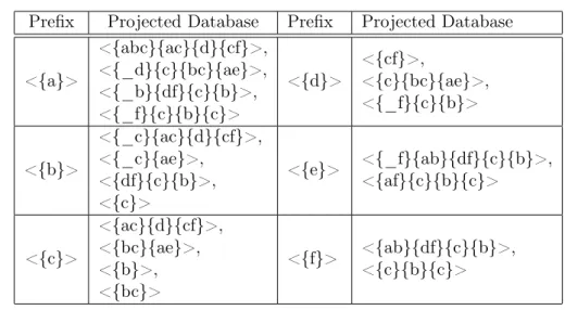
PrefixSpan algorithm In 2001, Pei et al., [41] proposed PrefixSpan algorithm (Prefix-projected sequential pattern mining). This algorithm is built upon the concept of sequential database projection proposed in FreeSpan algorithm [24]. PrefixSpan extends FreeSpan by taking into account the testing of prefix subsequences and the projection of their corresponding postfix subsequences into separate projected databases.

Definition 1.1.9. (s-projected database)

Let us consider a frequent sequence s in a sequential database S_D. The s-projected database, denoted by S_D|s, is the collection of all suffixes of the sequences in S_D with respect to the prefix s.

Example 1.1.4. (s-projected database)

Table1.5displays some projected databases of the sequential database in Table 1.1with respect to 1-prefixes.

1.1. Sequential pattern mining (SPM) Prefix Projected Database Prefix Projected Database

<{a}> <{abc}{ac}{d}{cf}>, <{_d}{c}{bc}{ae}>, <{_b}{df}{c}{b}>, <{_f}{c}{b}{c}> <{d}> <{cf}>, <{c}{bc}{ae}>, <{_f}{c}{b}> <{b}> <{_c}{ac}{d}{cf}>, <{_c}{ae}>, <{df}{c}{b}>, <{c}> <{e}> <{_f}{ab}{df}{c}{b}>, <{af}{c}{b}{c}> <{c}> <{ac}{d}{cf}>, <{bc}{ae}>, <{b}>, <{bc}> <{f}> <{ab}{df}{c}{b}>, <{c}{b}{c}>

Table 1.5 – Projected database of Table1.1

PrefixSpan uses depth-first enumeration to explore the search space of sequential patterns. The first step, that is common to most of sequential pattern mining algorithms, is to scan the sequential database in order to calculate the support of the single items and thus to obtain the frequent singletons (1-sequential patterns). Next, it performs a depth-first enumeration starting from the frequent singletons. For a given sequential pattern s of length k, PrefixSpan first builds the projected database with respect to the prefix pattern s. It then scans the projected database of s, counts the support values of items and detect frequent items to be appended to s, and thus (k+1)-frequent patterns are formed. After that, the algorithm repeats this step recursively to find all frequent sequential patterns.

The advantage of the projected database concept is that the projected databases keep shrin-king where a projected database is smaller than the original one because the subsequences that are projected into a projected database are only the postfix subsequences of a frequent prefix. Ho-wever, its disadvantage is that it scans the database repeatedly and builds projected databases, and these repeated scans could be of a high cost. Certain techniques were proposed for reducing the number of projected databases [25]. One of these techniques is the pseudo-projection where the sequence databases can be held in main memory in order to avoid redundancy in the postfixes of the projected databases. Instead of constructing a physical projection all the postfixes, they use pointers referring to the sequences in the database as a pseudo-projection.

Despite this disadvantage that could be limited when the size of the sequential database as well as the length of patterns are reasonable, prefixspan is a well known and widely used algorithm in various domains like multi-dimensional sequential pattern mining and sequential pattern mining with time constraints.

1.1.2 SPM algorithms using vertical representation

Sequential pattern mining algorithms using a vertical database representation adopt the pattern growth-based approach. Some of these algorithms are SPADE [64], SPAM [6], Hirate and Yamana [28], and CMAP [14]. Among these algorithms, SPADE is the first algorithm proposed in this context.

SPADE algorithm

In 2001, Zaki et al., [64] proposed the first algorithm that uses a vertical database format for mining sequential patterns, SPADE algorithm (Sequential Pattern Discovery using Equivalence classes). This algorithm is inspired by ECLAT [66] and CHARM [65] algorithms for mining frequent itemsets. SPADE uses based search techniques and simple joins. The lattice-based approach is used to decompose the original search space, the lattice, into smaller pieces, the sub-lattices, that can be processed in the main memory in an independent manner. It usually requires three scans of the sequential database in order to obtain the frequent sequential patterns. The algorithm works as follows. First, it scans the database and transforms it from horizontal to vertical database format where each item is associated with its corresponding id-list. An example of horizontal-to-vertical database transformation is the horizontal database displayed in Table

1.1that is transformed into the vertical database displayed in Tables1.3and1.4. Then, it scans the vertical database, reads the id-list of each item and calculates the support value of the item which represents the total number of sid’s found in the id-list. The items that have a support value above the predefined minsup are considered as frequent singletons. After generating these singletons, the algorithm performs a vertical-to-horizontal transformation in order to recover the original horizontal database by grouping the items with the same sid and in an increasing order of eid. Table1.6shows the horizontal database recovered from the vertical id-lists of items. Then, it forms a list of all 2-sequences for each sid in order to generate frequent 2-sequential patterns. The support of a frequent 2-sequential patterns is calculated by joining the id-lists of the two items forming this sequence by making a join on the same sid where the eid of the first sequence occurs before the eid of the second sequence. The generated frequent 2-sequential patterns are used to construct the lattice. The number of frequent 2-sequential patterns could be large which makes the lattice formed out of it quite large to fit in the main memory. Therefore, the lattice is decomposed into different equivalence classes such that the sequences having the same prefix items belong to the same equivalence class. Then, frequent (k +1)-sequential patterns are explored from frequent (k)-sequential patterns via temporal joins using either breadth-first or depth-first enumerations. Then id-lists of the frequent (k)-sequential patterns are joined to calculate the support values and therefore generate frequent (k + 1)-sequential patterns. Longer frequent sequences are generated similarly until no more frequent sequences could be generated. In the breadth-first enumeration of the equivalence classes of the lattice, the equivalence classes are generated in a recursive bottom-up manner where all the child classes at each level are explored before moving to the next level. For example, in order to generate frequent (k + 1)-sequences, all the (k)-sequences have to be already explored. While in depth-first enumeration of the equivalence classes of the lattice, all equivalence classes for each path in the search space are explored before moving to the next path of the search space. For example, all the (2)-sequences as well as the (k)-sequences have to be already explored in order to generate frequent (k + 1)-sequences.

sid (Item, eid) pairs

1 (a, 1), (a, 2), (b, 2), (c, 2), (a, 3), (c, 3), (d, 4), (c, 5), (f, 5) 2 (a, 1), (d, 1), (c, 2), (b, 3), (c, 3), (a, 4), (e, 4)

3 (e, 1), (f, 1), (a, 2), (b, 2), (d, 3), (f, 3), (c, 4), (b, 5) 4 (e, 1), (g, 2), (a, 3), (f, 3), (c, 4), (b, 5), (c, 6)

1.2. Multi-* data The advantage of SPADE algorithm is that it requires only three scans of the database in order to generate all the frequent sequences which makes it faster than GSP algorithm which requires multiple database scans to generate all the frequent sequences. In addition, SPADE uses simple temporal join operation on id-lists.

After the proposition of SPADE algorithm, other sequential pattern mining algorithms using vertical database representation were proposed across years [6,5,62,14,62].

SPADE as well as other sequential pattern mining algorithms using vertical representation have several advantages. The main advantage is introducing the concept of lists. The id-list structure is simpler than other structures used in horizontal databases such as complicated hash-tree structures. In addition, as the length of a frequent sequence increases, the size of its id-list decreases, resulting in faster joins. The vertical database representation also facilitates the process of support calculation. The support of a pattern is the total number of sid’s in the id-list and the support of a (k + 1)-sequence is calculated through the intersection of the id-lists of the two frequent (k)-sequences that form this sequence ; therefore, it avoids the repetitive database scans required for calculating the support of the sequences. It also saves the information not only about the sequences where the items occur but also about the events that show when these items occur. However, a disadvantage is that when the cardinality of the set of transactions is very large, the intersection time of the id-lists becomes costly.

SPAM [6] and Bitspade [5] algorithms propose a bitmap representation of the database with efficient support counting which optimizes the id-list structure and thus makes these algorithm faster than SPADE. However, the limitations of these two algorithms are that they generate a large number of candidate patterns and that the join operation made in order to generate the id-list of each of these candidate patterns could be a process of high cost. Therefore, CM-SPADE and CM-SPAM algorithms [14] were proposed to improve these two algorithms by introducing the co-occurrence pruning in order to reduce the number of joins. These algorithms initially scan the database to create the co-occurrence map (CMAP) that stores frequent 2-sequences. Then for each pattern explored in the search space, if its last two items are not frequent 2-sequences, then this pattern is discarded without making the join operation to generate its id-list. This process of verifying if the pattern is frequent before generating its id-list saves time and reduces the cost of the mining process and thus makes these algorithms faster than the previous ones.

In this section, we have presented the related work in the domain of sequential pattern mining by presenting important algorithms from different categories.

1.2

Multi-* data

Voluminous amounts of digital data are created and collected on daily basis. This data may not always come from the same data source and may not always be homogeneous ; however, it could be heterogeneous representing different kinds of data and thus forming complex datasets. The heterogeneity of this data lies in the fact that it could be provided by various data sources, could be represented as different data dimensions and could have different relations among the sources or dimensions. This heterogeneity results in what we call multi − ∗ data which briefs the multiple kinds of data contained in this complex dataset. In this section, we describe the various kinds of multi-* data, and in the following section, we focus on the mining of such data.

1.2.1 Multi-source data

A data source is simply any source that provides data. It could be a file, web data, a database or a data warehouse. Multi-source data represents data collected from multiple data sources.

These different data sources can be classified into sources of homogeneous structures, named homogeneous data sources, and others of heterogeneous structures, named heterogeneous data sources. The data in a data source is known as local data with respect to this data source and the data of all data sources is known as global data.

Homogeneous data sources

Homogeneous data sources are the sources that have the same data structure which is the way of organizing the elements of data as well as the way they are related to each other. In other words, the data sources contain the same data elements with the same names, data types and data structures, and they are usually distributed among different locations. Table 1.7 displays two data sources providing academic data of students from two different schools. These different data sources are homogeneous as they have the same structure and provide the same kind of data elements which are the averages and the ranking of students among the class.

Another example of homogeneous data sources is provided in [12] where the data represents information about patients’ trajectories provided by different hospitals.

Student-id Average(/20) Rank(/25)

123 12 15

126 15.8 3

124 11.5 18

122 7 22

(a) School 1

Student-id Average(/20) Rank(/25)

132 8.5 24

135 16.1 2

138 13.5 11

131 10 19

(b) School 2

Table 1.7 – Students’ academic data from two schools

Heterogeneous data sources

Heterogeneous data sources are the sources that have heterogeneous structures. Heteroge-neous data sources can be classified into two types. The first type is when the sources have heterogeneous data models at the local level. Data model heterogeneity, which is also considered as schematic and data heterogeneity, occurs when the same data is stored and represented in different ways causing data inconsistency and leading to obtain heterogeneous data sources al-though these sources have the same data nature with the same semantics. Example of these data inconsistencies are as follows. There could be conflicts of synonyms and homonyms among dif-ferent data sources. A synonym conflict is when the same data element is represented in difdif-ferent names among different data sources. A homonym conflict is when different data elements have the same name among different data sources. There could also be differences in the data types, precision or scale ; for example, a data element could be defined as integer in one data source and as float in another one. In addition, there could be structural differences among different data sources on the level of their objects ; for example, it could have a single value in one data

1.2. Multi-* data source and multiple values in another one. There could also be a problem of missing or conflicting data in the data values recorded such as having two different values for the same object in two different data sources due to errors or differences in the underlying semantics [8].

The second type of heterogeneous data sources is when the sources are related but different. In other words, the various data sources have heterogeneous data models and provide different data. The data sources are related as they provide semantically relevant data ; however, each data source has its own role in providing one or more kinds of data. They may share some data types or names of data elements ; however, they do not represent the same elements and they have different semantics. Combining these various data sources together allows forming a heterogeneous dataset whose data heterogeneity and the relations existing among its different data sources make it rich, informative, understandable and thus interpretable.

An example of heterogeneous data sources in the domain of e-commerce is as follows : one data source could provide descriptive data about the customers, another data source could provide data about their past purchases, and a third data source could provide descriptive data about the products that are purchased by the customers. Each data source gives different kinds of data about the customers and their purchasing process which allows extracting various and rich information.

The main challenge in extracting information from multi-source data lies in how to manage such kind of heterogeneous data coming from different sources efficiently and with limited com-plexity. Multi-source frequent pattern mining has been a topic of interest, and many research works across years have proposed various techniques to mine multi-source data in order to obtain useful and rich information that serves the scientific objectives and desired outcomes. The related work in the domain of multi-source pattern mining is detailed in section1.3.1.

1.2.2 Relational data

When the data are heterogeneous and of different natures, they represent relational data, and they can thus be represented as multiple relational database tables (relations). These data are called relational data, and they are also referred to as multi-relational data in the literature. Figure1.1displays an example of a relational database about customer’s purchases of products from companies. This example shows that there are different kinds of relations existing among different tables.

Relational data allows extracting various and rich information that comes from various da-tabase tables, and the process of mining frequent patterns from this kind of data is known as relational pattern mining, also called in the literature multi-relational pattern mining. A lite-rature review of the various approaches proposed in the domain of relational pattern mining is detailed later in section1.3.2.

1.2.3 Multi-dimensional data

Data can consist of different data fields, where each field corresponds to a set of measured properties that are referred to as features, attributes, or dimensions [1]. This kind of data is called multi-dimensional data. An example of multi-dimensional data is as follows. Let us consider a data source providing descriptive data about the food products purchased by customers in a market ; this source provides different data dimensions to describe each product such as : product name, category, fabrication date, expiry date, etc. Each data dimension could be represented as several attributes describing different products.

Figure 1.1 – Relational database

Frequent patterns could be generated from multiple data dimensions which allows obtaining patterns that contain various kinds of information. Such kind of frequent patterns are called frequent multi-dimensional patterns [45,12].

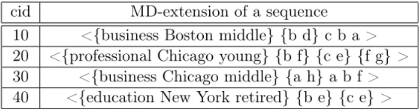
In many applications, one data dimension of the multi-dimensional data represent data se-quences forming a multi-dimensional sequential space. For example in the domain of customer purchase, the customer purchase history is associated with customer group, address, time, age group and others. This specific kind of multi-dimensional data is called multi-dimensional se-quential data containing multi-dimensional sequences [45, 63, 12, 50, 47, 46, 29, 56, 22]. Pinto et al., [45] were the first to introduce the notion of a multi-dimensional sequence, and Table 1.8

displays an example of their database that contains multi-dimensional sequential data where cid represents the customers ids.

cid Customer Group City Age Group Product Sequence 10 business Boston middle < {bd}cba > 20 professional Chicago young < {bf }{ce}{f g} > 30 business Chicago middle < {ah}abf > 40 education New York retired < {be}{ce} >

Table 1.8 – A multi-dimensional sequential database [45]

In certain cases, there could be background knowledge about the data dimensions which allows translating this knowledge into a data hierarchical structure. When there are several attributes representing each data dimension, the hierarchical structure of data is called a data taxonomy. We name this kind of data as multi-dimensional data with hierarchical structure. Figure 1.2

1.3. Mining multi-* data

Figure 1.2 – A hierarchy of food products [18]

In other cases, data dimensions could represent descriptive data about one or more other data dimensions. This descriptive data provide certain contexts to the other dimensions which allows giving broader understanding of the data within which it is associated. This kind of data is called contextual data. The contextual data could be associated to data sequences giving contexts to each sequence forming contextual sequential data [48]. An example of a contextual sequence is : cs : {young, f emale} < {ab}c >. The contextual data represent a young female, and the sequential data represent {ab} then c.

Many research works in the literature have been proposed to mine different kinds of multi-dimensional data. In section1.3.3, we discuss the literature review of multi-dimensional sequential pattern mining, multi-dimensional pattern mining using hierarchical structures and contextual pattern mining.

From the previous description of the various kinds of data, we can understand that the term multi-* data refers to the following kinds of data : multi-source, multi-dimensional and relational data. Although they are different kinds, they are related to each other and the data in a dataset could sometimes be classified as one or more of these kinds of data. For example, we could have two data sources where each source provides more than one data dimension, and these sources could have relations among them ; in this case, the data is multi-source, relational and multi-dimensional at the same time. Such a dataset has more complex and heterogeneous structure than other datasets containing data of one kind ; consequently, it can be viewed and thus managed from different perspectives. Various approaches have been proposed across years for mining these different kinds of data. In the following section, we present the related work in mining these different kinds of data.

1.3

Mining multi-* data

Mining multi-* data has always been a topic of interest as the challenge lies not only in generating interesting frequent patterns from these data but also in the efficiency and the low complexity of the mining process. In the following subsections, we present the related work in the domains of multi-source, multi-dimensional and relational pattern mining respectively.

1.3.1 Multi-source pattern mining

Multi-source pattern mining is a topic of pattern mining concerned in mining data coming from different data sources. This topic has gained a great interest as it represents data in real applications. Various approaches have been proposed to mine this kind of data. These approaches are divided into two main categories. The first category is integrating data from all data sources

and mining them together in order to generate frequent global patterns. The second category is mining frequent patterns from each local data source, named frequent local patterns and then integrating all the local frequent patterns of all data sources together. In the following subsections, we present some interesting research works from the two categories of multi-source pattern mining.

Mining multi-source data in an integrated manner

Multi-source data integration involves aggregating data from different data sources to a cen-tralized data source and perform a single mining process on this cencen-tralized source in order to extract patterns that are globally frequent among all the local data sources.

Some works proposed approaches to mine data that is integrated in a centralized source in order to extract frequent patterns that include information from all the sources.

Data fusion is the process of integrating data from homogeneous data sources into a single source, and a single mining process is performed on this data to generate frequent patterns. An example of this approach is the multi-sensor data fusion proposed in [32]. Multi-source data fusion is an intelligent synthesis process of remote sensing image data from multiple sources and generating accurate, complete and reliable estimation and judgement. Their proposed approach first collects the data from different sensors and then eliminates the data redundancy and conflicts that could exist among this multi-source data in order to generate useful information from this integrated data. This approach is proved to be efficient in this domain as it can improve the reliability of remote sensing information and can help in decision making and planning.

This approach of combining multiple data sources together and mining them in a single mining process has several drawbacks that proves its inefficiency. Integrating multi-source data in a single source could cause a considerable cost due to the data integration. In addition, the number of items in each itemset or sequence increases which augments the length of these itemsets or sequences resulting in higher complexity of the mining process. Integrating multi-source data into a single database may destroy some important local information from local data sources that reflects the distributions of patterns. For example, such kind of specific information would be lost : "85% of the branches within a company agree that a customer usually purchases sugar if he/she purchases coffee" [67]. Another possible limitation of this approach is the data protection and privacy rules that could allow transferring the resulting patterns without allowing to transfer the data. Besides, this approach considers that each data source has the same weight (importance) and doesn’t take into consideration that different data sources could have different weights where a data source could have a bigger contribution to the mining process and its results than another one.

Mining Multi-source data in a distributed manner

In order to overcome the limitations of the previously described approach, other works propo-sed to mine different data sources in separate mining processes to obtain frequent local patterns and then integrate all the frequent local patterns generated from each mining process in order to obtain frequent global patterns.

In 2009, Peng et al., [43] proposed three algorithms in order to mine sequential data contai-ning sequences of events that are represented in different domains where a domain contains events occurring within a predefined time window. The first algorithm proposed a naive approach which mines multiple data sources where each one is represented in a database. In this algorithm, the multiple sequence databases are integrated as one sequence database, and it is mined using

tra-1.3. Mining multi-* data ditional sequential pattern mining algorithms such as PrefixSpan algorithm [25]. This algorithm is then proved to be costly and inefficient due to the data integration. Therefore, two other algorithms were proposed to overcome the drawbacks of the first one. The second algorithm, IndividualMine algorithm, consists of two phases : the mining phase and the checking phase. In the mining phase, sequential patterns in each sequence database are mined using a traditional sequential pattern mining algorithm. Then in the checking phase, sequential patterns from all domains are integrated in order to generate multi-domain sequential patterns which has the same concept as multi-source sequential patterns. In this algorithm, each domain should individually perform sequential pattern mining algorithms, which incurs a considerable amount of mining cost. Therefore, in order to further reduce this cost, they propose a third algorithm, the Propa-gatedMine algorithm, in which those sequences that are likely to form multi-domain sequential patterns are extracted from their sequence databases. The PropagatedMine algorithm consists of two phases : the mining phase and the deriving phase. In the mining phase, the algorithm performs a sequential pattern mining using traditional sequential pattern mining algorithms in a starting domain and then propagates time-instance sets of the mined sequential patterns to the next domain until all domains are mined. In the deriving phase, the algorithm extracts those sequences with occurrence time equal to those of the time-instance sets propagated.

The third algorithm is proved to be the most efficient one among the three algorithms as it reduces the complexity and thus the cost of the mining process. Therefore, it is a good and efficient approach for mining this kind of data that is homogeneous among different data sources ; however, the concept of pattern propagation is infeasible when the data among different data sources are heterogeneous. In addition, this approach considers that different data sources have equal contributions to the resulting patterns and it thus doesn’t take into consideration that a data source could contain data that is of bigger weight and thus is more important than the other.

Zhang et al [67] proposed an approach for generating global exceptional patterns in multi-database mining applications where each data source is represented in a separate multi-database. An exceptional pattern is a pattern that is highly supported by only few data sources ; in other words, such a pattern has a very high support value in some data sources and zero support value in others which allows to have a high global support value. This kind of patterns reflect the individuality of different data sources. The proposed approach, named Kernel Estimation for Mining Global Patterns (KEMGP), considers that different data sources have different contributions to the resulting global patterns and thus they have different minimal supports. It mines each data source and generates its frequent local patterns, and then it identifies the local exceptional patterns of interest from these local patterns. In their work, they also describe another kind of patterns, called suggesting patterns [67,43] that is based on the votes done by the databases in order to decide for the global patterns among all local ones. They define the suggesting patterns as the patterns that have fewer votes than a minimal vote ; however, they are very close to the minimal vote where the minimal vote is determined by users or by experts. If a local pattern has votes that are equal to or greater than the minimal vote, then the local pattern is said to be a global pattern, named a high-voting pattern. While if a local pattern has votes that are less than the minimal vote but are very close to the minimal vote, then it is called a suggesting pattern that could sometimes be useful for decision making [43]. The concept of "suggesting patterns" that is introduced and defined in this work is an interesting concept as it represents patterns that are on the margin of global ones and that weren’t far from being global.

The approach proposed in this work is efficient as it allows identifying the importance of a pattern not only locally in a specific data source but also globally on the level of all data sources. However, the approach works strictly on homogeneous data sources where a global