HAL Id: hal-02600757
https://hal.inrae.fr/hal-02600757
Submitted on 16 May 2020HAL is a multi-disciplinary open access archive for the deposit and dissemination of sci-entific research documents, whether they are pub-lished or not. The documents may come from teaching and research institutions in France or abroad, or from public or private research centers.
L’archive ouverte pluridisciplinaire HAL, est destinée au dépôt et à la diffusion de documents scientifiques de niveau recherche, publiés ou non, émanant des établissements d’enseignement et de recherche français ou étrangers, des laboratoires publics ou privés.
hydrological model: the influence of frozen soil
Y. Tondu
To cite this version:
Y. Tondu. simulation of the Paris 1910 flood with a lumped hydrological model: the influence of frozen soil. Environmental Sciences. 2010. �hal-02600757�
TRITA-LWR Degree Project 11-09 ISSN 1651-064X
ISRN KTH/LWR/Degree Project 11-09 ISBN 55-555-555-5
S
IMULATION OF THE
P
ARIS
1910
FLOOD
WITH A LUMPED HYDROLOGICAL MODEL
:
T
HE INFLUENCE OF FROZEN SOIL
Yohann Tondu
ii © Yohann Tondu 2010
Degree Project in Hydraulic Engineering
Department of Land and Water Resources Engineering Royal Institute of Technology (KTH)
SE-100 44 STOCKHOLM, Sweden
Reference should be written as: Tondu, Y. (2010) “Simulation of the Paris 1910 flood with a lumped Hydrological model : The influence of frozen soil”, Trita 11-09, 120p.
iii
S
UMMARYSvenska
Denna uppsats handlar om simulationen av en översvämning i Paris år 1910. Efter en kort redogörelse av denna händelse och dess konsekvenser beskrivs regnflödes hydrologiska modellen, GR4J, som nu används till att förutse översvämningar av Seinebassängen. I nästa del presenteras resultaten av simulationen för översvämningen 1910 framtagen av GR4J på huvudbassängen i Seine vid Paris och 4 av dess underbassänger. När dessa resultat visade sig misslyckade, togs en ny
hypotes fram om den möjliga inverkan av tjäle på
översvämningsformationen. Således togs en frostmodul fram, kopplad till en jord temperatur modell med luft temperaturer som inläggsdata. Resultaten av simulationen för översvämningen 1910 framtagen av GR4J kopplad till frostmodulen är slutligen presenterade. Sammanfattningsvis, nya perspektiv är presenterade för att fortsätta forskningen.
Français
Ce mémoire a pour sujet la simulation de la crue qui inonda Paris en 1910. Après une brève présentation de cet évènement et de ses conséquences, GR4J, le modèle hydrologique pluie-débit aujourd’hui utilisé par les services de prédiction des crues sur le bassin de la Seine, est décrit. Le chapitre suivant présente les résultats obtenus par ce modèle en simulation de la crue de 1910 sur les bassins de la Seine à Paris et de 4 de ses sous-bassins. Comme ces résultats n’étaient pas satisfaisants, l’hypothèse d’une possible influence du gel sur la formation de la crue a été formulée. Un module gel a donc été développé, couplé avec un modèle de simulation de la température du sol à partir de la température de l’air. Enfin, les résultats des simulations de la crue de 1910 obtenus par GR4J couplé à ce module gel sont présentés. En conclusion, de nouvelles pistes d’études sont présentées pour poursuivre les recherches.
English
This thesis deals with the simulation of the flood that took place in Paris in 1910. After a brief presentation of this event and its consequences, GR4J, the lumped hydrological model that is now used in flood prediction on the Seine basin is described. The next part is presenting the results of the 1910 flood simulation obtained by GR4J on the main Seine at Paris basin and on 4 of its sub-basins. As these results were disapointing, a new hypothesis was developed about the possible influence of frozen soil on the flood formation. A frost module is thus developed, coupled with a soil temperature model using air temperatures as input data. The results of the 1910 flood simulation by GR4J coupled with the frost module are finally presented. In the conclusion, new perspectives are presented to continue the research.
v
A
CKNOWLEDGEMENTSI would like to thank my two French supervisors Vazken Andréassian and Charles Perrin for their help, their advices and their incredible benevolence. I would also like to thank the whole Hydrology team in CEMAGREF for their support and their happiness. It was really nice working with you. I would then like to thank the whole DIREN team for providing the data and helping with the calculations.
Thank you also to my Swedish supervisor, Hans Bergh, for his help. I would also like to thank Peter Brokking, Eva Lindhal, Nawal Safey and Mme. Arbeille who all helped me to get this internship.
Finally, I would like to thank all my friends and family for their unconditional support during those tempestuous times. I wouldn’t have finished this thesis without you.
vii
T
ABLE OF CONTENT Summary ... iii Svenska ... iii Français ... iii English ... iii Acknowledgements ... vTable of content ... vii
Table of French institutions and abbreviations ... x
Abstract ... 1
1 Introduction : the 1910 flood ... 2
1.1 The 1910 flood causes ... 2
1.2 The 1910 flood consequences ... 2
1.3 If the Flood happened today ... 10
1.4 Purpose of the study ... 10
1.5 Method ... 10
1.6 Conclusion ... 11
Other References ... 11
2 The GR4J model ... 12
2.1 Model description ... 12
2.1.1 Precipitation and Evapotranspiration ... 12
2.1.2 Recharge and Discharge of the production store ... 12
2.1.3 Percolation ... 14
2.1.4 Unit Hydrographs ... 15
2.1.5 Routing store and water exchange ... 16
2.1.6 Total flow at the bottom of the basin ... 17
2.2 Method to run the model ... 17
2.2.1 The different steps ... 17
2.2.2 Evaluation Criteria ... 18
2.2.3 Influence of the initial values of S and R... 18
2.2.4 Software used ... 20
Appendix 2.1 : Calculation of Ps in the GR4J model... 20
References ... 22
3 Modelling the 1910 flood with the GR4J model ... 23
3.1 The simulation of the 1910 flood ... 23
3.1.1 Data ... 23
3.1.2 Method ... 23
3.1.3 Results ... 24
3.1.4 Discussion ... 24
3.2 Taking into account the water reservoirs ... 26
3.2.1 Influence on the GR4J model... 27
3.2.2 Model of reservoirs ... 28
3.2.3 Influence of the model on the calibrated parameters' values ... 29
3.2.4 Application of the model to the 1910 flood ... 29
3.2.5 Data ... 29
3.2.6 Method ... 29
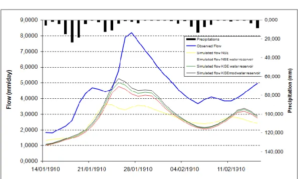
3.2.7 Results ... 30
3.2.8 Discussion ... 31
3.3 Discussion on the statistical tools used in the model ... 31
3.3.1 Decomposition of the Nash-Sutcliffe Efficiency ... 31
viii
3.3.3 Application on the replication of the 1910 flood... 33
Appendix 3.1 : Calculation of the 1909-1910 average precipitation on the Paris Austerlitz basin ... 36
References ... 37
4 Test on the sub-basins ... 38
4.1 Data and Method for tests on the sub-basins ... 38
4.1.1 Data ... 38 4.1.2 Method ... 38 4.2 Loing at Episy ... 39 4.2.1 Results ... 39 4.2.2 Discussion ... 39 4.3 Marne at la-Ferté-sous-Jouarre ... 42 4.3.1 Results ... 42 4.3.2 Discussion ... 43 4.4 Seine at Bazoches-lès-Bray ... 44 4.4.1 Results ... 44 4.4.2 Discussion ... 44 4.5 Yonne at Courlon-sur-Yonne ... 45 4.5.1 Results ... 45 4.5.2 Discussion ... 47
4.6 Simplified propagation model ... 47
4.6.1 presentation of the model... 48
4.6.2 Data ... 49
4.6.3 Method ... 49
4.6.4 Results ... 49
4.6.5 Discussion ... 52
4.7 Conclusion ... 53
5 The Frost Hypothesis ... 54
5.1 Theory of frozen ground ... 55
5.1.1 Frost definition and types ... 55
5.1.2 factors influencing frost formation ... 55
5.1.3 frost hydraulic and hydrologic effects ... 56
5.2 Presentation of the frost modules ... 56
5.2.1 The linear module ... 57
5.2.2 The Z&G module ... 58
5.3 Test of the new model including frost modules ... 59
5.3.1 Data ... 59 5.3.2 Method ... 59 5.3.3 Results ... 59 5.3.4 Discussion ... 67 5.4 Conclusion ... 70 References ... 70
6 Soil temperature models ... 72
6.1 Modeling soil temperature ... 72
6.1.1 Factors influencing the soil temperature ... 72
6.1.2 The different models ... 73
6.2 Selected models ... 73
6.2.1 Bocock model ... 73
6.2.2 Paul et al. model ... 76
6.2.3 Plauborg model ... 77
6.2.4 Lindström et al. model ... 78
ix 6.3.1 Data ... 78 6.3.2 Method ... 80 6.3.3 Results ... 81 6.3.4 Discussion ... 93 6.4 Conclusions ... 94 References ... 95
7 Test of the frost module on the 1910 flood ... 97
7.1 Data ... 97
7.2 Method ... 97
7.3 Results ... 98
7.3.1 Marne at Ferté basin ... 99
7.3.2 Seine at Bazoches basin ... 102
7.3.3 Seine at Paris Austerlitz basin ... 103
7.4 Discussion ... 106
7.5 Conclusion ... 107
Reference ... 108
8 Conclusion and perspectives ... 109
8.1 Rain undercatch ... 109 8.1.1 Principle ... 109 8.1.2 Data ... 110 8.1.3 Method ... 110 8.1.4 Results ... 110 8.1.5 Discussion ... 112
8.2 Delays and modified precipitations ... 112
8.2.1 Delays ... 112
8.2.2 modification of the precipitations ... 113
8.2.3 Data ... 113
8.2.4 Method ... 113
8.2.5 Results ... 113
8.2.6 Discussion ... 115
8.3 Linking error and temperature ... 116
8.3.1 Data ... 116
8.3.2 Method ... 116
8.3.3 Results ... 116
8.3.4 Discussion ... 118
x
T
ABLE OFF
RENCH INSTITUTIONS A ND ABBREVIATIONSCEMAGREF : French national research institute in environment. This thesis was done in internship in their laboratories.
DIREN : Regional Direction for Environment. Organism that is in charge of the flood prediction in Paris and that owns many archives related to the flood flow in 1910.
GR4J : Hydrologic Rainfall-Runoff model used throughout this study
for flow simulation.
Grands Lacs de Seine : Organism that manages the 4 water reservoirs upstream of Paris. Météo France : French national meteorological institute.
1
A
BSTRACTIn 1910, Paris experienced its biggest flood in the 20th century. In 2010, for the anniversary of this event – supposed to happen every 100 years ! – the flood prediction model that is now used on the Seine basin was tested on its simulation,… and failed to reproduce the observed flood volume. This paper will try to explain, and correct, such disappointing results. Many hypotheses have been tested and based on their results, it has been decided to develop a frost module in order to assess the influence of this phenomenon – that is not taken into account by the lumped hydrological model that is used – on the flood formation. A soil temperature model using air temperature as input data was also designed because soil temperature data were not available in 1910. The addition of the frost module did not, however, bring many improvements to the 1910 flood simulation because frost is a too rare phenomenon on the Seine basin for the module to be correctly calibrated. However, new perspectives are presented to continue the research on this phenomenon.
Key words : Paris 1910 flood ; Lumped hydrological model ; Rainfall-Runoff model ; Frost
2
1
I
NTRODUCTION:
THE1910
FLOODIn winter 1910, from January to March, Paris experienced its biggest flood of the 20th century with the Seine river reaching a maximum level
of 8,62m at the Paris Austerlitz station (around 8m more than the normal level) on Januray, 28th. The 1910 flood was also named “crue
centennale” (100 years flood) because it was estimated that it had a probability of 1/100 to happen in any given year. Thus 2010 was a very special anniversary for this flood and this is how the subject of this thesis was launched in order to assess whether it could be possible to predict the 1910 flood today with the available hydrologic models.
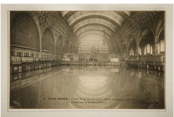
This introduction will briefly describe the 1910 flood, its causes –to the extent of the current knowledge - and its effects. A last part will present what the consequences of a similar flood would be nowadays and how the main institutions are prepared for such an event. Most of the data and figures that will be introduced here were presented by the different invited speakers during the colloquium organized by the Société
Hydrologique de France (French Hydrologic Society) on March, 24th, 25th
2010 about this particular event. The pictures are all coming from the archives of the Bibliothèque Historique de la Ville de Paris (Paris Historical Library).
1.1 The 1910 flood causes
In 1909, the summer and the last trimester were particularly rainy with unusual precipitation levels that saturated the soil with water.
In January 1910, two episodes of heavy rains were reported. The first one took place from January, 18th to 21st with unusually strong
precipitations on many parts of the basin. Because of the saturated soil – and maybe other factors – the Seine and its tributaries reacts immediately with unusual water levels. The peak flows of the most rapid tributaries like the Yonne river reaches Paris in a few days and the water level in Paris Austerlitz raises. Peak flows of the other tributaries like the Marne river and the Seine are expected later, around January, 28th.
But from January, 23rd to January, 25th a second episode of precipitations
happens that results in a second peak flow on all the basin’s rivers. Around January, 26th, the second peak flows of the rapid tributaries meet
the first peak flows of the slower tributaries and of the Seine. The simultaneity of those 2 events will then result in the maximum flow of the 1910 flood that will reach Paris on January, 28th.
After 10 days of increase, the water level in Paris Austerlitz will then decrease from January, 29th but won’t reach a normal level before March
1910 with the occurrence of other peak flows during February 1910.
1.2 The 1910 flood consequences
A plan of the flooded areas in Paris is displayed on figure 1.1. Of course during the 1910 flood, the water got over the river’s bank and flooded the streets, but it also infiltrated in the underground tunnels like the subway lines and reaches other parts of the city that were not very elevated like, for example, the Saint-Lazare station (Fig. 1.2). Monuments (Fig. 1.3 and 1.4) and garden (Fig. 1.5) were also flooded as long as other strategic places like stations (Fig. 1.6) or the deputies chamber (Fig. 1.7). But the most famous symbol of the 1910 flood still is the Alma bridge zouave statue on which Parisians measure the water level and that will be flooded till the shoulders (Fig. 1.8).
3
Fig. 1.1 Plan of the Flooded areas in Paris. In Orange the places where water infiltrated the caves, in blue, the places where it reached the streets.
4
Fig. 1.3 Notre-Dame de Paris cathedral
The subway lines are rapidly flooded and unusable, especially near to the Seine. To move around the city, the Parisians thus mostly use horses as most of the modern energy transports are also unable to work in those conditions (Fig. 1.9). In some quarters, barks will even be used (Fig. 1.10) - the deputies will reach their chamber this way (Fig. 1.7). Finally, small plank footbridges will be built in the most flooded street to allow pedestrians to cross them (Fig. 1.11).
Only one person died because of the flood. It nevertheless had huge social and economical consequences with 20 000 of the 80 000 buildings of the capital being flooded and 150 000 people stricken. The flood did not strike Paris only and it is more than 200 000 people that immigrated from the suburb to the capital where first aid was more organized. The cost of the flood was estimated at 400 million francs-or for direct damages plus 50 million francs-or spent on aids which in total is equivalent to 1,4 billion euros (Ambroise-Rendu M. cited in DIREN, 2010).
5
6
7
Fig. 1.6 Inside of the Orsay station – that will become the Orsay museum.
8
Fig. 1.8 The Alma bridge with the zouave statue.
9
Fig. 1.10 A bark in the Surcouf street
10
1.3 If the Flood happened today
Today, the Seine banks in Paris have been raised to the 1910 flood water level in order to limit the spreading of water in the capital if a similar flood had to happen again. The Seine bed has also been enlarged and now it would necessitate 110% of the 1910 flow for the water to reach the same level. Furthermore, several water reservoirs were built in order to limit the peak flow – even if in the case of a flood similar to the 1910 one, they will not have much effect. Finally, the different emergency scenarios designed by the ORSEC (Civilian Security Response Organization) are all based on the 1910 flood : the R1.0 scenario represents the case of 100% of the 1910 flow, the R0.6, 60%, the R1.15, 115%. In 2010, an exercise was launched ans it was possible to predict the peak flow 72 hours in advance with the different hydraulic and hydrologic models.
Furthermore, the main institutions have designed emergency plans based on the different scenarios cited above. The RATP which is in charge of the public transport in the Parisian region thus have the obligation to protect the underground subway network in order to re-open it after the flood. around 100 pumps have thus been placed in the areas liable to flooding. Furthermore, in case of a high flood, all the entrance of the 42 stations (out of 297) situated in vulnerable areas would be sealed with bricks and concrete that are already in stocks. In a similar way, the health care services have sesigned scenarios for hospital evacuation in flood cases. Finally, the Defense quarter (biggest business quarter in Europe) has also designed plans with the use of independent electric generator to allow for a minimum computer service during 36 hours.
Despite all this, it was estimated that, if the R1.0 scenario (100% of the 1910 flows) was happening today, 820 000 people would be flooded in Paris and its small suburb only, 1 220 000 would lack electricity and 1 500 000 would lack drinkable water. In Paris and its suburb, 90% of the areas liable to flooding are already built, thus adding an industrial risk, for example by chemical pollution of the water. In the Ile-de-France region 800 000 jobs would be threaten because of the damages with a cost equivalent to 30% of the regional GDP (Growth Domestic Product). In 1998, les grands lacs de Seine (cited in DIREN, 2010) estimated that such a flood would have a total cost of more than 12 billion euros.
1.4 Purpose of the study
In order to be able to predict a similar flood in the future, this study aims at testing the following hypotheses as explanations of the 1910 flood and of the difficulties encountered in its simulation :
No particular causes
Influence of the water reservoirs
Influence of the model evaluation criterion Propagation of the error from selected sub-basins Influence of frost
and from these tests conclude on the 1910 flood causes and integrate them in the hydrological model used in flood simulation.
1.5 Method
The evaluation of the different hypotheses listed above has been made with the GR4J model (“modèle du génie rural à 4 paramètres, journalier”) that is described in chapter 2. Different modules that are also described in the study were also used when necessary.
11
1.6 Conclusion
The 1910 flood thus was the largest flood of the 20th century. If it
happened in very specific conditions, each winter there is one chance out of 100 that it would happen again. In this case, there would be even more harmful social and economical consequences than in 1910 because of the urbanization.
It is thus important to be able to predict such an event as soon as possible in order to allow for a better application of the different emergency scenarios. This study will thus focus on the simulation of the 1910 flood with GR4J which is the hydrologic model that is now used in flood prediction on the region. Indeed, if it manages to reproduce the flood satisfactorily then the model can be expected to accurately predict a similar event much more in advance than any hydraulic model because GR4J uses rain as input data while hydraulic models use upstream flows. In the next chapter, the GR4J model will be described. Then it will be used on the 1910 flood to assess the way it can simulate it on the main Paris Austerlitz basin and then on several sub-basins. Finally, in front of the poor results obtained in simulation, it was thought that frost could have played a role by reducing water infiltration in the soil. A new frost module will thus be designed - coupled with a soil temperature model using air temperature as input data – in order to take into account its influence on hydrology. This module will then be tested on the 1910 data.
Other References
DIREN (2010) Conditions de déclenchement de la crue de 1910. Online at
http://www.ile-de-france.ecologie.gouv.fr/spip.php?article
243
[accessed on 20/11/2010]12
2 T
HEGR4J
MODELThe GR4J model which stands for "modèle du Génie Rural à 4 paramètres Journalier" (i.e. daily model for rural engineering with 4 parameters), is a daily lumped rainfall-runoff hydrological model. From precipitations and evapotranspiration data, it gives an estimation of the water flow at the outlet of the studied basin. It is used in many applications at the basin scale, especially a modified version called GR3P is currently being used for flood forecasting in the Seine basin..
The first version of the GR4J model was developed empirically in the early 1980s at CEMAGREF and has been modified several times over the last decades. The version presented in this chapter is described by Perrin et al. (2003). GR4J is a rather simple model with only four free parameters (i.e. parameters that are to be calibrated before getting results from the model) but it gives results similar to more complex models. Some modules can however be used to take into account some specificities like, for example, water reservoirs influence or snow melt.
2.1 Model description
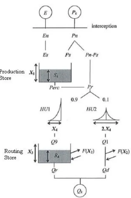
GR4J is an empirical lumped model designed at the basin scale. It is not directly linked to physics and uses stores to represent the overall water behaviour. It is illustrated in figure 2.1.
All the equations of this chapter are provided by Perrin et al. (2003) and Perrin et al. (2007). In those equations, all the volumetric terms are expressed in mm, by dividing them by the catchment area as GR4J is a lumped model considering the basin as a whole and averaging every data on its surface.
2.1.1Precipitation and Evapotranspiration Pk and E are the input data :
Pk (mm) reprensents the areal precipitation depth at day k averaged over the surface of the basin.
E (mm) is the daily potential evapotranspiration
The net precipitation Pn is equal to 0 if E>Pk and equal to Pk-E
otherwise. The net evapotranspiration En is equal to 0 if Pk>E and equal
to E-Pk otherwise.
2.1.2Recharge and Discharge of the production store
If Pn>0, the net rainfall water is then divided and a part of it will go in the production store, if En>0 water is taken from this production store. This store stands for the humidity or moisture of the basin and is often confused with the soil although there is no direct link. It is aimed at dividing the rainwater - in a part that will actually reach the rivers and a part that will go back to the atmosphere by evapotranspiration or percolate later - by taking into account the past conditions over the basin (past precipitations and evapotranspiration). The production store is basically a stock of water Sk (in mm at the beginning of day k) that will
increase or decrease due to rainfall and evapotranspiration. Part of this water will also percolate to the rivers.
13
Fig. 2.1 scheme of the GR4J model principle (source : Perrin et al. (2003)
If Pn>0, the production store is thus recharged by a part of the rainfall Ps expressed in mm. Ps is given by :
1 1 1 2 1 1tanh
1
tanh
1
X
Pn
X
S
X
Pn
X
S
X
Ps
k k (Eq. 2.1)Where X1 (in mm) is the maximum capacity of the production store and
is the first parameter of the GR4J model.
CEMAGREF (1991) provides a brief development of the calculation that leads to this result for Ps. During a day, it is considered that only a
14 fraction
2 1 21
X
S
of the net precipitation Pn will be brought to the production store, and that this fraction will fall on the store following a uniform temporal distribution along the day. We can then integrate the mass-balance equation of the production store under those conditions on a day to obtain Sk+1 function of Sk. Ps is then deduced by the
equation : Ps = Sk+1 – Sk. As an example, the calculation of Ps is shown
in annexe 2.1.
If En>0, the production store is discharged of a quantity of water Es expressed in mm and given by the equation :
1 1 1 1tanh
1
1
tanh
2
X
En
X
S
X
En
X
S
S
Es
k k k (Eq. 2.2)There again, CEMAGREF (1991) offers an explanation for this calculation. It is considered that only a fraction
1 12
X
S
X
S
of the net evapotranspiration En is actually effective, and that the effect will follow a continuous temporal distribution along the day. The mass-balance equation of the production store is then integrated on a day to obtain Sk+1 function of Sk and Es can then be deduced with Es = Sk+1-Sk.
Finally, the new store stock S' (mm) is then :
S' = Sk + Ps – Es (Eq. 2.3)
2.1.3Percolation
The percolation Perc is a quantity of water (in mm) that is taken from the production store to end up in the rivers. This term is small related to store content and was actually not present in the first versions of the GR4J model. It was added later as a corrective term that gives better results (i.e. results that fit more to the reality) especially for low flows. It is given by the equation :
4 1 4 1'
9
4
1
1
'
X
S
S
Perc
(Eq. 2.4)And thus the new store stock Sk+1 becomes :
15
2.1.4Unit Hydrographs
The upstream water Pr (in mm) that reaches the routing part of our model is thus :
Pr = Pn – Ps + Perc (Eq. 2.6)
This water is then divided : 90% will be routed via a unit hydrograph UH1 and a routing store and the other 10% will be routed by a symmetric unit hydrograph UH2.
Those hydrographs mainly aim at delaying the arrival of water to the outlet by taking into account and weighting the importance of the previous days' precipitations. They have been designed empirically. The 90%-10% division is also an empirical result. Making this splitting variable from basin to basin, with the introduction of a 5th free parameter
does not bring any improvement (Perrin, 2000).
Unit hydrographs ordinates are calculated using the S-curves SH1 and SH2 : 4 4 2 5 4 1 0 0 0 ) ( 1 X t if X t if X t t if t SH (Eq. 2.7) and :
4 4 4 2 5 4 4 2 5 42
1
2
2
2
1
1
0
2
1
0
0
)
(
2
X
t
if
X
t
X
if
X
t
X
t
if
X
t
t
if
t
SH
(Eq. 2.8)Where X4 is the time base for UH1 expressed in days and is a parameter
of the GR4J model that needs to be calibrated. We can then define UH1 and UH2 :
UH1(j) = SH1(j) – SH1(j-1) (Eq. 2.9)
UH2(j) = SH2(j) – SH2(j-1) (Eq. 2.10)
With j an integer.
Finally, at day k, Q9 and Q1, the water flows (in mm/day) that are getting out of the 2 hydrographs are given by the equations :
16
l jj
k
j
UH
k
Q
1)
1
Pr(
)
(
1
9
,
0
)
(
9
(Eq. 2.11)
m jj
k
j
UH
k
Q
1))
1
Pr(
)
(
2
(
1
,
0
)
(
1
(Eq. 2.12)Where l = int(X4)+1 and m=int(2X4)+1 with int(.) the integer part.
2.1.5Routing store and water exchange
The routing store is characterised by Rk, the stock of water at the
beginning of the day k (in mm) and by X3 its capacity (in mm) that is a
parameter of the model. The routing store is used to simulate the flow dynamic and the recession of a flow peak some days after a heavy rain. It smoothes the flow curve resulting from the model.
The exchange term applied to the routing store replicates the water exchange with other basins due to groundwater aquifers. This exchange F, that can be positive or negative, is given by the equation :
2 7 3 2
X
R
X
F
k (Eq. 2.13)Where X2 is the exchange coefficient in mm. It is the last parameter of
the model.
The stock of water in the routing store R' then becomes :
R'= max(0; Rk + Q9(k) + F) (Eq. 2.14)
Some of this water Qr (in mm/day) is released from the routing store to reach the flow at the outlet of the basin :
4 1 4 3'
1
1
'
X
R
R
Qr
(Eq. 2.15)CEMAGREF (1991) also describes this calculation. If, within a day, we call Q(t) the water flow exiting the routing store at time t, R(t) the stock of water in this store at time t and Δt the duration of one day, then the result shown above is coming from the integration of the mass-balance equation in the routing store supplemented by the empirical equation :
4 3 5
4
)
(
)
(
tX
t
R
t
Q
.And the stock of water in the routing store becomes :
17
2.1.6Total flow at the bottom of the basin
The flow Q1 also exchanges water with the others basins with the same exchange term F. The resulting amount of water Qd (in mm/day) that reaches the river is thus given by :
Qd = max(0; Q1(k) + F) (Eq. 2.17)
Finally the amount of water flowing at the outlet of the basin at day k, Qk (in mm/ day) is :
Qk = Qr + Qd (Eq. 2.18)
2.2 Method to run the model
2.2.1The different steps
In the ideal situation, to run the model, we need two data sets at two different time periods of at least 5 years. The data needed are daily precipitations and evapotranspiration (in mm) averaged on the basin - using reference stations where the data are available, as well as daily flow values at the outlet of the basin (in m3/s.).
On the first data set, the model will be calibrated : the four parameters will be given values that give the best results when matching the simulated and the observed water flow values. The length of the calibration period can have a small influence on the calibrated values of the free parameters but this influence becomes negligible when the calibration period is long enough (at least 5 years). Generally, the longer the calibration period, the more robust the calibration as more hydrological events happening on the basin are likely to occur and thus are likely to be taken into account in the calibration process (Perrin, 2000).
On the second data set, the values of the four parameters are used and the model is run to control that those values give good results when matching the observed and simulated flows in order to validate the calibration.
The process is summarized in figure 2.2.
It can be interesting at the end of this process to reverse it, using the second data set to calibrate the model and the first one to validate it. It can then be seen how the different parameters values evolve. A big difference can then have many interpretations : change in the basins conditions, unreliability of our model, other unknown factors,…
18
2.2.2Evaluation Criteria Calibration
The model has 4 parameters that are summarized in table 2.1 (Perrin et al., 2007)
During the calibration process we will vary those 4 parameters in order to find the combination that reaches the best fit between the simulated and the observed water flows. Several evaluation criteria exist to assess this fit between the 2 ranges of data (see for examples, Perrin, 2000 and Perrin et al., 2003). Generally the Nash-Sutcliffe Efficiency (NSE) is used. Its formula is given by Nash and Sutcliffe (1970) :
n k o k o n k k s k o x x x NSE 1 2 , 1 2 ; , ) ( ) ( 1
(Eq. 2.19)Where n is the number of values, xo,k is the observed value at time k (the
observed flow), xs,k is the simulated value at time k (the simulated flow),
and μo is the mean of the observed values. NSE is often given in %.
NSE varies between -∞ and 1. If it is negative, then the simulated results are worse than the mean observed values and a constant would give better results than the model which is thus considered useless. If the NSE is equal to 1 then the observed and simulated values are exactly equal. Thus during the calibration process, one must try to reach an NSE as close as possible to 1 i.e. as high as possible. In this case the calibration process is an optimization of the 4 parameters X1, X2, X3 and
X4 to maximize NSE.
Other criteria exist using, for example, the square root or the logarithm of flows in the NSE formula as observed and simulated values. The use of those different criteria will be discussed in chapter 3.
Validation
In the validation process, the same criteria or new ones can be used to assess the quality of the calibration of our 4 parameters on a new data set. Several criteria can be used at that step - whereas the calibration is generally made to optimize one criterion only even if, nowadays, more and more works develop a multi-criteria approach.
2.2.3Influence of the initial values of S and R
Before running the model, for calibration or control, initial values of S and R (i.e. S0 and R0) must be set. Le Moine (2008) has shown that the
setting of those values could influence the efficiency of the model. In practice, we initialize the values of S0/X1 and R0/X3 arbitrarily between 0
and 1. The influence of those initial values are shown on figure 2.3. Table 2.1 GR4J parameters and their statistical values
Parameter Description Median Confidence Interval at 80%
X1 Production store capacity (mm) 350 100 to 1200
X2 Exchange coefficient (mm) 0 -5 to 3
X3 Routing store capacity (mm) 90 20 to 30
19 0,000 0,100 0,200 0,300 0,400 0,500 0,600 0,700 0,800 0,900 1,000 01/01/94 01/05/94 01/09/94 01/01/95 01/05/95 01/09/95 01/01/96 Date S /X 1 Initial value : 0 Initial value : 1
Fig. 2.3 filling ratio S/X1 evolution with time in the GR4J model with the parameters values : X1=776,90mm, X2=0,48mm, X3=75,41mm, and X4=3,62 days for initial values of S/X1 of 0 and 1..
It can be seen in figure 2.3 that the filling ratio curves are almost identical after a certain amount of time (around one year here) whether their initial value S0/X1 was set to 0 or to 1. Indeed Le Moine (2008)
shows that after some time, S/X1 will reach a state of steady evolution
independent of initial values. Ideally, the model should be run after this state is reached but that can take some time, especially in case of important production store capacity (X1) which will allow a larger
variability for the store level S. The same results can be obtained with R0/X3 although the routing store generally has a smaller capacity, thus
allowing less variability and a quicker reach of the steady evolution state. Thus, in practice, when running the model for calibration or for control, no result is accounted for during a defined period – warm-up period - which is only used to settle the values of S and R. During this period, no observed values of flows are necessary since S and R are only influenced by precipitations and evapotranspiration. The flow values (simulated and observed) belonging to this period are not taken into account in the calculation of the efficiency of the model – for example with the NSE criterion - or for any other calculation.
Le Moine (2008) has designed a specific method for initialisation of S0/X1 that allows the model to reach the state of steady evolution more
quickly and thus to reduce the warm-up period –or give better results than an arbitrary S0/X1 value with an equal warm-up period. However,
Perrin (2000) using a model very similar to GR4J for a test on 595 calibration on 17 different basins concludes that after one year of initialisation, only 8% of the parameters values change with different initial values of S0/X1 and R0/X3.
In this study, the influence of the initial value set to S0/X1 and R0/X3 will
20
this whole study, the values S0/X1 = 0,60 and R0/X3 = 0,70 will thus be
taken with a warm-up period of one year. 2.2.4Software used
To run the GR4J model, two softwares were mainly used in this study : Microsoft Office Excel – named Excel in this study, and Compaq Visual Fortran – named Fortran in this study.
Excel
All the formulas – to run the model and calculate its efficiency - are put in different cells. The data are completed by the operator and the calculation is instantaneous. For Calibration, the solver tool was used.
Fortran
Fortran is a programming language that is able to open and read many different files in a very quick time. The program used in this study is also able to handle other models than GR4J with different numbers of parameters. Additional modules can also be integrated in those models to simulate snow influence in the basin.
A "step-by-step" optimization method is used in the program for calibration (Mathevet, 2005, Perrin, 2000). For GR4J, the four parameters X1, X2, X3 and X4 are given an arbitrary initial value. The
efficiency criterion (e.g. NSE) is then calculated based on those parameters values. One by one, each parameter value is then added and subtracted a constant step ΔX and the efficiency criterion is recalculated with this different set of parameters values and compared to the previous result. The set of parameters values that give the best result is then selected and taken as a basis for another iteration of the optimization process and so on. The variation step ΔX is raised to accelerate the process when several consecutive improvements are found in the same direction. Reversely, it is diminished if, during an iteration, no better result than the initial set of values could be found in order to allow for a more precise research around this set of values. The optimum is said to be found when the variation step ΔX becomes lower than the minimum variation step decided in advance.
The efficiency criteria's variation with the parameters values is generally simple, without secondary optimum, in the GR4J model. The "step-by-step" method has thus proven to be effective both in optimization time and in results compared to other methods – implying several initial parameters values, for example (Perrin, 2000).
Appendix 2.1 : Calculation of Ps in the GR4J model.
This calculation is shown as an example of the developments that have led to the equations of the GR4J model. It is largely inspired from CEMAGREF (1991).
Within day k, we call P(t) the net amount of water falling per unit of time on the basin at time t and S(t) the volume of the production store at time t. We consider that P(t) follows a uniform distribution along the day. Thus
u Pn t
P , with Pn the total net precipitation during the day and
u the duration of one day. We consider that only a fraction
2 1 21
X
S
of P(t) actually reaches the production store. Finally we don't take into account the percolation that is calculated separately.
21 2 2 1 2 2 1 2 1 2 1 S X Pn Pn dS u t d S uX Pn u Pn dS dt dt u Pn X S dS With
h
X
Pn
1
2 1
we get by integration :
hPn
S
Argth
hPn
t
S
Argth
Pn
h
u
t
(
)
(
0
)
We then have S(0) = Sk (initial condition) and S(u) = Sk+1. Then for
t = u :
h
Pn
th
hPn
S
S
h
Pn
th
hPn
S
hPn
S
Argth
h
Pn
th
hPn
S
hPn
S
Argth
hPn
S
Argth
h
Pn
k k k k k k k1
1 1 1We can then replace h by Pn X12
and calculate Ps which is the amount of water brought to the production store during the day so :
22 1 1 2 1 2 1 1 1 1 1 1 2 1 1 1 1 1 1 X Pn th X S X S X Pn th X Ps X Pn th X S X Pn th X S S S X Pn th X Ps S S Ps k k k k k k k k
References
CEMAGREF (1991) Hydrologie appliquée aux petits bassins ruraux, CEMAGREF, Groupement d'Antony, division : Hydrologie.
LE MOINE, N. (2008) Le bassin versant de surface vu par le souterrain : une voie d'amélioration des performances et du réalisme des modèles pluie-débit ? , UNIVERSITE PIERRE ET MARIE CURIE PARIS VI, CEMAGREF ANTONY HBAN. 348 p.
MATHEVET, T. (2005) Quels modèles pluie-débit globaux au pas de temps horaire ? Développements empiriques et comparaison de modèles sur un large échantillon de bassins versants. Ecole Nationale Du Genie Rural Des Eaux Et Des Forets, Cemagref Antony, Hban. 463 p.
NASH, J. E. & SUTCLIFFE, J. V. (1970) River flow forecasting through conceptual models part I -- A discussion of principles. Journal of
Hydrology, 10, 282-290.
PERRIN, C., MICHEL, C. & ANDREASSIAN, V. (2007) Modèles hydrologiques du Génie Rural (GR). CEMAGREF, UR Hydrosystèmes et Bioprocédés.
PERRIN, C., MICHEL, C. & ANDREASSIAN, V. (2003) Improvement of a parsimonious model for streamflow simulation.
Journal of Hydrology, 279, 275-289.
PERRIN, C. (2000) Vers une amélioration d'un modèle global pluie-débit au travers d'une approche comparative. Institut National Polytechnique de Grenoble, Cemagref Antony, Qhan, 530 p.
23
3 M
ODELLING THE1910
FLOOD WITH THEGR4J
MODELThe GR4J model has proved in the past years to be rather robust and reliable and is now at the basis for the flood forecasting model used in the Seine basin by the DIrection Régionale de l'ENvironnement (DIREN : regional direction for environment). At the occasion of the anniversary of the "crue centennale" (100-years flood), the DIREN tried to run the model to simulate this phenomenal flood. This was the first time that the model was run on those data. The experiment and its results are described in the first part of this chapter.
In front of the poor results obtained during this simulation, and before further investigations, the model - especially the calibration process - was questioned in order to find an explanation to the large difference between observed and simulated values. Two tests were thus conducted about artificial influences between 1910 and 1994 and statistical criteria used for optimization, based on previous studies showing that those factors could influence the results of models (Payan, 2007, Gupta et al., 2009). The experiments and their results are described in the second and third part of this chapter.
3.1 The simulation of the 1910 flood
The experiment was conducted with the GR4J model as described in chapter 2 without any modification of its structure, the aim being to assess its efficiency in modelling the 1910 flood.
3.1.1Data
The following data were used :
For Calibration : observed flow values at Paris Austerlitz (in m3/s) as
well as precipitation, and evapotranspiration values (in mm) averaged on the Seine basin upstream of Paris Austerlitz – of a surface of 43800 km². for conversion of volumetric values. Precipitation and evapotranspiration values covered the period from January 1st 1994
to December 31st, 2009. Flow values covered the period from
January 2nd, 1995 to December 31st, 2009. Those data were provided
by the "Banque Hydro" (French national data base for hydrological data).
Observed flow values at the station of Paris Austerlitz in m3/s from
November 1st, 1909 to February 28th, 1910. Those data were given
by the DIREN. The peak flow was traditionally believed to be around 2400 m3/s which happened to be inconsistent with the data
available upstream and downstream from Paris. In the set of data used this mistake was corrected and the peak flow was estimated at 2649 m3./s.
Precipitation and evapotranspiration (in mm) averaged on the whole Seine Basin upstream of Paris Austerlitz and covering the period from January 1st, 1909 to December 31st, 1910. Those data were
extracted from paper archives available at DIREN or provided by Météo France (French National Institute for meteorology). The calculation method for the average precipitation on the basin is described in appendix 3.1.
3.1.2Method
The GR4J model as described in chapter 2 was used with the Excel software.
For calibration, the range of data covering the period from 01/01/1994 to 31/12/2009 was used, with one year (1994) used to settle the values
24
of S and R and not taken into account for the efficiency computation (one year model warm-up). The 4 parameters X1, X2, X3 and X4 were
calibrated so as to maximize the NSE criterion calculated on flow values (NSE calibration).
The parameters calibrated as seen above were used to run the model with the 1909 – 1910 data. The year 1909 was used to settle the values of S and R and the simulation covered the period from 01/01/1910 to 28/02/1910.
Finally, a calibration of the model on the 1909 – 1910 period was made by maximizing the NSE criterion calculated on the flow values. The first year (1909) was used to settle S and R values and was not taken into account in the calculations.
3.1.3Results
The model calibration on the period 1994 – 2009 gave the parameters values presented in table 3.1. When using those parameters on the 1909 – 1910 period as described in part 3.1.2 the efficiency results given in table 3.2 were obtained
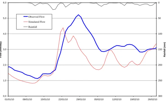
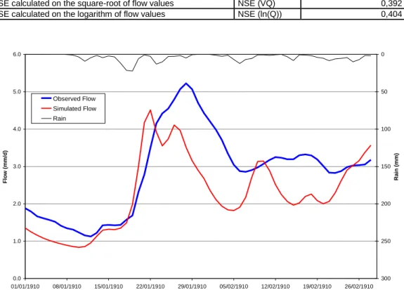
The observed and simulated flow values are shown on figure 3.1.
By simple integration of the curve presented on figure 3.1, the observed and simulated volumes of water that flowed at Paris Austerlitz between 01/01/1910 and 28/02/1910 are calculated : the observed volume is 7,3483.109m3 and the calculated volume is 5,6326.109m3, and the
difference between observed and simulated volumes thus represents 23,35% of the observed volume.
Finally, after calibration on the 1909 – 1910 period as described in part 3.1.2, the parameters took the values presented in table 3.3.
3.1.4Discussion
The Nash-Sutcliffe efficiencies obtained on the period covering January and February 1910 after calibration on the 1994 – 2009 period, are all very low (below 0,30) as we can see in table 3.2. The figure 3.1 also shows a large difference between simulated and observed flows with a clear underestimation by the model.
Table 3.1 parameters values after NSE calibration on 1994 - 2009
Parameter Unit Value after calibration
Production store capacity : X1 mm 777
Exchange coefficient : X2 mm 0,48
Routing store capacity : X3 mm 75
Time basis for UH1 : X4 days 3,6
NSE obtained with those
. 0,825
parameters on 1995 - 2009
Table 3.2 efficiency results obtained on the 1910 flood with NSE calibration on 1994 2009
Criteria Abreviation Result of simulation
NSE calculated on flow values NSE(Q) 0,229
NSE calculated on the square-root of flow values NSE (VQ) 0,227
25 0,0 1,0 2,0 3,0 4,0 5,0 6,0 01/01/10 08/01/10 15/01/10 22/01/10 29/01/10 05/02/10 12/02/10 19/02/10 26/02/10 F low ( mm /day) 0 50 100 150 200 250 300 Rainf all ( mm ) Observed Flow Simulated Flow Rainfall
Fig. 3.1 rainfall, observed and simulated flow from 01/01/1910 to 28/02/1910 with NSE calibration on 1994 – 2009
The underestimation of the flow can be directly translated in an underestimation of the level of the Seine river and of the water volume that flowed in Paris – the simulation lacking 23,35% of this volume i.e. more than 1,7 billions cubic meter of water between January 1st and
February 28th 1910. In case of such a natural catastrophe like the 1910
flood, it is important for the authority to be accurately informed in advance of the extent of the flood. Such an error in the simulation that would have led to a tremendous underestimation of the situation gravity is thus completely unacceptable.
There are three possible explanations to those very poor results : Data could be wrong.
The model can be unable to simulate such a flood, and will always give false results in those conditions of precipitation and evapotranspiration
There is something that happened in 1910 or between 1910 and 1994, that is not taken into account in our model, and that is leading to those wrong results.
The data source are rather well-documented and are less likely to be false than the model. It has thus been decided to investigate further the 2nd
and 3rd possibilities.
Table 3.3 parameters obtained after NSE calibration on the 1909 – 1910 period
Parameter Unit Value after calibration
Production store capacity : X1 mm 191
Exchange coefficient : X2 mm -0,19
Routing store capacity : X3 mm 302
Time basis for UH1 : X4 Days 6,4
NSE obtained with those
. 0,963
26
Finally it is interesting to compare tables 3.3 and 3.1. Table 3.1 gives relatively usual values for the parameters while in table 3.3, which actually replicate the flood with a very high NSE criterion, a huge diminution of the production store capacity, and a large augmentation of the routing store capacity can be observed. In a physical interpretation, by reducing the production store capacity, the model is allowing a faster saturation of the soil leading to increased run-off - and thus augmentation of water in the river at the end. By raising the routing store capacity, the model simulates a smoother response while reducing the loss of water into other aquifers (the exchange coefficient is negative). Those two values of the stores capacities are very unlikely, but they give clue on what must be looked for. An event, that would raise the runoff or lead to more water obtained from the soil, that is not taken into account in our model but that had happened in 1910, could explain those differences between observed and simulated values.
However, before investigating the possibility and consequences of such an event, and as a first preliminary approach, the model calibration method will be questioned. Especially, the influence of infrastructure changes on the basin between 1910 and 1994 and the statistical criteria used for optimization will be studied.
3.2 Taking into account the water reservoirs
In our previous experiment we have calibrated the model on the years 1994 – 2009 to use it on the years 1909 – 1910. One reason of the poor results we obtained could be that the conditions in the basin have changed between those two time periods so drastically that they could be considered as two independent basins.
In 1910, in the journal d'agriculture pratique of the French Académie
d'Agriculture (Academy of agriculture), Paul Descombes notes that after
the 1910 flood of Paris, a special budget for strive against inundation had been voted. 222 millions of ancient Francs (around 340 000 euros) would be allocated to constructions on the basin - rivers' beds enlargement and creation of water reservoirs - and 122 millions of ancient Francs (around 190 000 euros) would be allocated to reforestation (Descombes, 1910).
Four reservoirs were thus built in the second half of the 20th century on
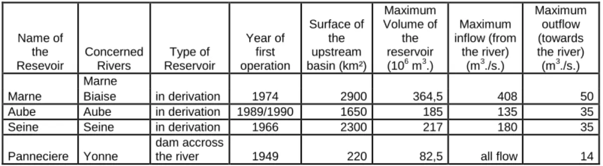
four rivers of the basin : Aube, Seine, Marne and Yonne. They are now managed by Les Grands Lacs de Seine institution created in 1969. Their location is shown on figure 3.2 and their main characteristics (Institution Interdépartementale des barrages-réservoirs des bassins de la Seine, 2010) are summarized in table 3.4.
The land cover changes are more difficult to appreciate as there is not much data available for 1910. Especially, whether the forest area in the basin has increased or decreased between 1910 and 1994 is not certain but this change is not assumed to be very significant. More significant could be the urbanization. Urban area in the basin has indeed certainly increased since 1910 due to population growth and national urbanization trend.
27
Fig. 3.2 The 4 major reservoirs on the Seine Basin (source : Institution Interdépartementale des barrages-réservoirs des bassins de la Seine, 2010)
3.2.1Influence on the GR4J model
Urbanization definitely has an impact on the hydrology of the basin by increasing the run-off coefficient of rain water. However as the basin was more urbanized in 1994-2009 than in 1910, the parameters calibrated on this first period should allow more run-off and thus an increased flow compared to parameters of 1910. Taking only the urbanization into account, calibration on 1994-2009 should thus lead to an overestimation of the flow in 1910. As the opposite problem is occurring, influence of changing urbanization won't be considered further.
More complicated is the assessment of other land covers changes between 1910 and 1994 and particularly of forests and their influence on the basin. Andreassian (2004) presents a review of many different paired-watershed experiments run worldwide in order to assess the link between basin hydrological behaviour and forestation/deforestation. If the results of those experiments appeared to be very variable, in case of flood, a deforestation of the basin will generally increase the flood peak and volume. However, this deforestation effect appeared to be significant only during the growing season of the year. Moreover, effect of reforestation –as it may have happened between 1910 and 1994 on the Seine basin, according to M. Descombes – appears in the few studies made about it to be very limited on floods in general, with "no effect at all on the large ones" (Andreassian, 2004, p. 12). As the 1910 flood of Paris can definitely be considered a large flood and that it happened in the dormant season (January), any possible deforestation or reforestation of the basin should not have any influence on it and thus the model should be able to replicate it even though it doesn't take into account land covers.
28
Table 3.4 characteristics of the four storages of the Seine basin
Name of the Resevoir Concerned Rivers Type of Reservoir Year of first operation Surface of the upstream basin (km²) Maximum Volume of the reservoir (106 m3.) Maximum inflow (from the river) (m3./s.) Maximum outflow (towards the river) (m3./s.) Marne Marne in derivation 1974 2900 364,5 408 50 Biaise
Aube Aube in derivation 1989/1990 1650 185 135 35
Seine Seine in derivation 1966 2300 217 180 35
Panneciere Yonne
dam accross
the river 1949 220 82,5 all flow 14
Finally, Oudin et al. (2008) in a study on hydrological impacts of land cover conclude that forest areas have less influence on the results of a water balance model than arable lands and that land cover data are much more informative on small catchments (<10 km²) – the Seine basin being 43800 km².
In front of all those results, it can be considered very unlikely that any land cover change would have a greater influence on model calibration – which, if leading to an underestimation of the 1910 flow by the model, would anyway be counter-balanced, to some extent, by the influence of urbanization that should lead the model to an overestimation - than the four reservoirs put in operation between the two time periods and that directly affect the rivers flows.
The enlargement of the rivers' beds doesn't change the flow of water in the rivers but only their levels. Thus, it won't have any influence on the model that works with flow values.
The influence of reservoirs on the GR4J model has been studied by Payan (2007).The production store capacity X1 appears to be the most
affected parameter. After calibration, in the presence of water reservoirs on the basin, a significant augmentation of its value can be observed compared to the value it had when there were not any reservoirs on the basin. The exchange coefficient X2 and the routing store capacity X3 are
moderately affected by the presence of reservoirs but whether an augmentation or a diminution of the values can be observed depends on the basin under study. Finally, the time basis for UH1 X4 is very little
affected by the presence of reservoirs and their influence can thus be neglected.
3.2.2Model of reservoirs
To diminish the influence of those reservoirs on the calibration on our data, one must try to integrate those reservoirs in the model in order to make the values after calibration of the parameters X1, X2, X3 and X4
more independent of the presence or absence of reservoirs on the basin. However, it is difficult to integrate site-located components such as water reservoirs in a lumped model like GR4J that considers the basin as a whole and that has no direct physical interpretation of its structure (Moulin, 2003, Payan, 2007, Payan et al., 2008).
Payan (2007) and Payan et al.(2008) have thus designed a model without describing the processes induced by the presence of reservoirs, but focusing on the volumetric variations of water stored in them. All the reservoirs are thus aggregated in a single store which volume Vk at the
beginning of day k is the sum of their respective volumes at that time. The variation ΔV = Vk+1 – Vk of this volume during day k is then