Ontario hydrometric network rationalization : statistical considerations.

(1)

Author Role:

Chaire en hydrologie statistique

Title, Monographic:

Ontario hydrometric network rationalization. Statistical considerations

Translated Title:

Reprint Status:

Edition:

Author, Subsidiary:

Author Role:

Place of Publication:

Québec

Publisher Name:

INRS-Eau

Date of Publication:

1996

Original Publication Date:

Juillet 1996

Volume Identification:

Extent of Work:

ii, 84

Packaging Method:

pages incluant 3 annexes

Series Editor:

Series Editor Role:

Series Title:

INRS-Eau, rapport de recherche

Series Volume ID:

470 Location/URL:

ISBN:

2-89146-436-2

Notes:

Rapport annuel 1996-1997

Abstract:

Rapport de la Chaire en hydrologie statistique soumis à M.M. Dillon Limited

Call Number:

R000470

(2)

Ontario Hydrometrie Network Rationalizatio/l

Statistical Considerations

(3)

Statistical Considerations

by:

Taha B.M.J. Ouarda

Peter F. Rasmussen

Bernard Bobée

Josée Morin

Chair in Statistical Hydrology

National Institute for Scientific Research, INRS-Eau

2800 Einstein, C.P. 7500, Sainte-Foy (Quebec) Gl V 4C7

submitted to:

M. M. Dillon Limited

BOX 1850 North York

Ontario, M2N 6H5

Rapport de recherche

NO

R-470

(4)

C

INRS-Eau,

1996

ISBN: 2-89146-436-2

(5)

M. M. DILLON Limited

F. Ivan Lorant

Jodi

L. Lougheed

Chair in Statistical Hydrology

INRS-Eau

Taha B.M.J. Ouarda

Peter F. Rasmussen

Bernard Bobée

Josée Morin

(6)

Table of contents ... i

Acknowledgments '" ...

ii

1 Introduction ... 1

2 Theoretical aspects ... 3

2.1 Classical record extension procedures ... 3

2.2 Application to the rationalization ofhydrometric networks ... 5

3 Rationalization methodology ... 7

3.1 Decision criteria ... 7

3.2 Identification of sub-regions ... 8

3.3 Description of the program REDUC ... 9

4 Application ... 13

4.1 Data base ... 13

4.2 Clustering analysis ... 15

4.3 Discussion ofresults ... 15

5 Conclusions ... 21

6 References ... '" ... 23

Appendix A Listing of the programs REDUC and ClAT ABLE ... 25

Appendix B Output of the program REDUC ... 31

(7)

This study was funded through a contract with the Division of Water Resources of M. M. Dillon

Limited, North York, Ontario. The authors of the present report gratefully acknowledge the input

and encouragement trom F. Ivan Lorant. The help ofJodi

L. Lougheed is also acknowledged.

(8)

1 Introduction

Traditionally, network designers have been concemed with accessing the suitability of potential

new sites for hydrometric monitoring. Today's budgetary constraints are imposing a new objective:

the elaboration of a rational strategy for reducing the CUITent hydrometric networks so as to

minimize the loss of information.

M. M. Dillon is currently involved in the process of rationalizing streamflow gauging stations for

flood management and water resource management in general for the Ontario Ministry ofNatural

Resources. The objective of M. M. Dillon's project is to define the requirements to the

hydrometric network for an adequate management of Ontario's water resources, and to develop

guidelines for adding and deleting stations. To select a general long-term, cost effective

monitoring strategy, M. M. Dillon is considering the data needs of the different users along with a

multitude of other criteria in the evaluation and rating of streamflow stations. Within this general

framework, the Chair in Statistical Hydrology at INRS-Eau has been asked to provide an

assessment of the statistical information content of the hydrometric stations in Ontario. The

statistical approach used in this study permits to identify, and eventually eliminate, stations whose

input to the total information is minimal, allowing in this way to minimize the loss of information

on a regional basis.

Various quantitative and qualitative criteria must be taken into account in the decision on which

stations to discontinue and which to maintain. Such criteria can include the following:

• size of the basin;

• record length;

• stability of control structures;

• accuracy of rating curve;

• number of demands for information during the last 10 years;

• estimated number of demands for information during the next 10 years;

• planned major projects;

• importance for the study of a particular problem such as floods;

• historical reasons;

(9)

• follow up of climatic changes and their impacts on hydrologie regimes;

• cost of operation and maintenance of the station; and

• accessibility of the station.

Although many factors must be considered, the contribution of INRS-Eau

rs

confined to analyzing

the statistical aspects of the rationalization of the hydrometric network of Ontario. A statistical

procedure for network rationalization was developed by Rasmussen et al. (1995) for the Ministry

of Environment of Quebec (Ouarda et al., 1996). The same procedure has been applied in this

study to the hydrometric network of the Province of Ontario. The final evaluation of the value of a

given station may involve an integration of the various criteria, of which statistical aspects

represent one particular element.

(10)

2 Theoretical aspects

In this section, the methodology for network rationalization based on the analysis of the

correlation between stations is briefly presented. The methodology will then be applied to the

streamflow gauging network of Ontario.

2.1 Classical record extension procedures

Short data series extension by means of linear regression has been frequently used in the past to

obtain series of equal length for use in the design and management of complex water resource

systems. Typically, one is interested in monthly flows, but other variables such as the annual

maximum daily discharge can also be considered. The HEC-4 program (U.S. Army Corps of

Engineers, 1971) was developed for this type of analysis.

An

improved version of HEC-4, the

software REMUS, was developed at INRS-Eau (perron et al., 1994). Sorne of the basic principles

for extending short records by means of regression are described in the following section. In a

subsequent section, these results are adapted to the case of the rationalization of hydrometric

networks.

We consider the case of two neighbouring gauging stations, possibly located on the same river.

Their corresponding watersheds are exposed to the same type of climate and more importantly

-often to the same meteorological events.

It

is therefore reasonable to assume sorne kind of

correlation between data at the two stations (annual flood data, monthly flow, etc.) Assume that

station Y has n) years of data (e.g. annual floods) and that station X has n)

+

n

₂

years ofwhich n)

are concomitant with the data observed at Y. This can be illustrated as follows:

(11)

We are interested in reconstructing information about flows at site

Y

for the n

₂

rrussmg years.

This can be done by simple linear regression of y on x, i.e. we assume that for the n

2 years,

Yi

can

be estimated as

(1)

Whether such synthetic data adds information or noise to one's knowledge of the statistical

characteristics of the y-series depends on several things. First of ail, it depends on the statistical

property one is interested in. Assume for instance that our interest is to estimate the mean value of

the variable

Y

as accurately as possible. Matalas and Jacobs (1964) showed that the mean value

ily

of the extended series can be expressed as

(2)

where YI is the average of

Yi

observed in period nI' and XI and

x

₂

are the averages of

Xi

observed

A

in periods nI and n

_{2 ,}

respectively. The parameter

J3

is the estimated regression coefficient. Based

on tbis formulation, it is possible to show (Cochran, 1953) that the variance of

il,

the mean value

estimator based on the extended series, is given by

(3)

where

(j~

is the population variance of

Y

and p is the population correlation between

X

and

Y. For practical use, these values may be replaced by their estimates based on the nI years of data. In

order to assess whether the extended series provides additional information on the variable Y, the

above variance must be compared with the variance obtained by simply estimating the mean trom

the nI observed values of

Y. The latter is given by

(j~

1 nI> and the condition for an improved

estimator (smaller variance) of the mean can be expressed as:

(4)

Hence, estimating the mean trom the extended series is profitable only if the correlation between

the two sites exceeds

(1 n) -

2It

l

/2.

If extension is desired at a particular site, one should identify

and use the auxiliary station in the network which leads to the minimum variance of the mean

value estimator. In general, this station must be highly correlated with the station of interest, and

there must be several years of concurrent data.

(12)

2 Theoretical aspects

5 If the variance of the y-series is of interest, one can proceed as in the case of the mean. Matalas

and Jacobs (1964) obtained the following expression for the unbiased variance estimator

&~

based

on the extended series:

(5)

where sx is the standard deviation estimate based on the entire x-series, and sX

_I

and

SYI

are,

respectively, the standard deviation estimates of X and Y based on the n) years of data. Moreover,

Matalas and Jacobs (1964) showed that the variance of the variance estimator based on the

extended series is given by

(6)

where

A,

B, and C are constants that depend on n) and n

₂

(see e.g. Vogel and Stedinger (1985)).

The first term on the right hand side is equal to the variance of the variance estimator based on the

n) years of y-data, and extension is therefore profitable wh en p

2 > ( - B ±

.,JB

2 -

4 AC) /2A.

It

should be noted that it is possible to consider the extension based on several neighbouring stations

(Moran, 1974). In that case, the correlation coefficient appearing in the above formula should be

replaced by the multiple correlation coefficient,

Pm'

and the period n) will be the period where aIl

stations have data. If

p

stations are considered as basis for the extension, then in the case of the

mean value estimator, the condition for an improved estimator is p!

>

p/(n) -

2). For annual

maximum and minimum flows, we have found that best results are generally obtained by

considering only one station.

2.2 Application to the rationalization of hydrometric networks

Looking at the rationalization problem from a purely statistical point ofview, one would choose to

eliminate stations that are highly correlated with another station in the network and in future years

reconstitute the missing data by regression techniques as described above.

It

should be

emphasized, however, that for the design of a rationalization strategy the problem is slightly

different from that described in the previous section. First of aIl, one cannot actually make the

extension at the present time, because future data (which is our interest) are not known. However,

one can assess the precision of, say, the variance of the mean value estimator (eq. 3) after a certain

number of years (assuming cr; and P remain unchanged and equal to present values). If the amount

(13)

of information contained in the extended senes is found satisfactory, O'ne may decide to

discontinue statiO'n

Y. It

is also possible tO' estimate the gain of waiting sO'me years before

abandO'ning a station.

The variO'us fO'rmulae presented in the previous section must be nrodified'

for

the case O'f

ratiO'nalizatiO'n. FO'r the purpO'se O'f illustration, cO'nsider the following data scenariO':

1960

1975

1995

2015

X:

***************

Y:

*****************************

The

tI*tI

indicates years fO'r which records exist. Here, nI is again the period O'f cO'ncurrent data at

the twO' sites, n

₂

is the future extension period, and n

₃

is a periO'd of additiO'nal data at site

Y. Hence, at statiO'n X there is data from 1975-95 and at station Y from 1960-1995. We consider an

extension hO'rizon of20 years, i.e. the periO'd from 1995-2015. In classical extensiO'n procedures, it

is always the shortest series that is extended. In the above case, it may be either X or Y, depending

on which criteria O'ne adopts for eliminating stations. In the case where statiO'n X is eliminated, O'ne

can use the formulae in the previO'us section by considering the period n

₂

+

n

₃

as the extensiO'n

periO'd. In the case where Y is eliminated, the formulae must be modified tO' accO'unt fO'r the period

n

₃

• It

can be shO'wn (Rasmussen et al., 1995) that the variance O'f the mean value estimatO'r at

station Y based O'n extension is given by:

(7)

Eq. 3 is a special case O'f tbis more general expressiO'n, obtained for n

₃

=

O. A similar expression

can be obtained fO'r the estimator of the variance (Rasmussen et al., 1995), but it is rather complex

and is not reported here.

EstimatiO'n O'f the mean with reconstructed data is profitable, compared tO' the use O'f only O'bserved

values, if:

(8)

(14)

3 Rationalization methodology

3.1 Decision criteria

A set of decision criteria must be defined to allow for the rational elimination of stations from the

network. Consider the case where budget cuts require k gauging stations be discontinued. Which k

stations among the

m

stations in the existing network should be selected? The number of possible

combinations of stations to abandon is given by the binomial coefficient

C(m,k).

For each

combination, one may compute an information figure according to which the combinations may be

ranked. Such a procedure would allow the identification of the best combination of sites to

eliminate, at least from a purely statistical point ofview.

The definition of a performance figure is a critical point and subject to several somewhat arbitrary

decisions. First, in order to use the approach described ab ove, it is necessary to define a time

horizon, n

₂

• The consequences of reducing the number of monitoring stations in the network is

not experienced immediately, but only after sorne years. One could try several time horizons and

examine the sensitivity of the optimal decision. Secondly, a performance figure that reflects the

amount of information one is likely to have available after n

₂

years must be chosen. For practical

comparison, this figure must be based on sorne kind of aggregated regional information.

It

is

important to identify the kind of information one is interested in. For example, one could choose

the inverse of the variance of the mean value estimator given by (7) as a surrogate for the amount

of information at a particular site. A global aggregated performance index

Ig (Q)

could be defined

for example as:

(8)

where

Q

is the basic variable of the rationalization, and

JÎ

is the mean value estimator. The

summation is carried out over ail stations in the network or in a pre-determined group of stations.

Note that the mean value of the logarithms of

Q

is considered. This is done to eliminate scaling

differences between sites. Therefore, a priori the sites in the network have equal importance, no

matter the size of their watersheds. For the sites where monitoring is continued, the best mean

(15)

value estimate will be based on n

₂

observed data, while at discontinued stations the variance will

be assessed using eq. 7. For each discontinued station, the best auxiliary station for record

extension is sought among the m-k remaining stations. After having examined all possible

combinations of station removal, one can identify the one that has minimum Ig (Q). The procedure

can be easily implemented on a computer.

It

should be strongly emphasized that the above procedure depends on the choice of the basic

variable. Quite ditferent results may be obtained if one considers for example annual floods and

annual minimum tlows. Renee, the variable of interest should be carefully selected keeping the

objective of the network in mind. It may also be preferable to perform the analysis with ditferent

variables and make sorne compromises in the choice of stations to eliminate.

3.2 Identification of sub-regions

Given the large size of the Ontario hydrometric network, it is desirable to pre-classify the network

in smaller geographical regions. The boundary of regions can be determined using a tree-clustering

algorithm as suggested by Bum and Goulter (1991). The correlation coefficient between the data

of two sites can be used to quantify the similarity between these sites. If many variables are of

interest, a weighted average can be used. The similarity between two sites

i

and

j

can be defined

as:

K

f·

_IJ

=

"IDkf,k··

_L.J

_,IJ

(9)

k=\

where

K

is the number of variables being considered (annual minimum tlows, annual maximum

tlows, and annual mean tlows, for example), ID k is the weight associated with the variable

k,

and

rk,ij is the correlation between sites

i

and

j

for the variable

k.

The distance between two groups, X

and Y, containing respectively nl< and ny sites can be defined by the following average linkage

clustering distance:

(10)

It

should be noted that, as a particular case, groups X and Y may contain only one site each. When

used in a rationalization context, clustering allows us to identify groups of sites that are highly

correlated. The final rationalized network should ideally contain stations from aIl identified groups

(16)

3 Rationalization methodology

9 of stations.

It

is obvious that, if aIl stations of a particular group are eliminated, it will no longer be

possible to extend data within that group in order to improve the estimates of the mean and the

variance. Consequently, the best approach consists in studying each of the identified groups

separately.

3.3 Description of the program REDUC

The program REDUC was developed to automatize the rationalization of hydrometric networks

(see Appendix A). The program was developed in the MATLAB environment and can only be run

if the software MATLAB and certain MATLAB Toolboxes are available. The various steps in the

computations performed by REDUC are briefly described in this section.

REDUC provides an answer to the following question: "If the objective is to eliminate k stations

among n stations in a particular region, which choice of k stations will minimize the performance

index, Ig ?" In the first stage, aIl possible combinations of k stations among a total of n stations are

identified. The number of combinations is given by the binomial coefficient:

C

k

=

_n!

n

k!(n-k)!

(11)

where

!

is the facto rial operator.

In the second stage, the index Ig is computed for each one of the possible

C~

combinations. The

combination leading to the lowest value of Ig is identified. For the analysis of a particular

combination, we proceed as follows: The n stations of the region are first split into two groups:

the first group contains the k stations proposed for elimination and the second group contains the

(n - k) stations to be conserved. The best estimate of the mean value of the variable of interest

(minimum, mean, or maximum) after n

₂

years is then identified. In this application, the value of the

horizon of estimation is fixed to n

2 =20 years. A set of results is also produced for n

2 =

10 years.

For the (n - k) stations to be conserved, the best estimate is obtained directly from observed data,

i.e. historical record and additional record to be acquired du ring the next n

2 =

10 years.

For each discontinued station, the variance of the mean is computed on the basis of observed data

and,

if

profitable, of reconstituted data. The program REDUC determines which station among the

(n - k) to be conserved should be used as an auxiliary station for reconstitution of information. As

(17)

explained above, this choice usually depends on the correlation between eliminated and auxiliary

stations, and the length of the common period of record.

Since quantiles of flow variables are often of interest, additional information concerning precision

estimation is computed by REDUe.

An

approximate expression for the estimation precision of

flood quantile estimates (and other variables as weil) is given by:

(12)

where n is the number of available observations, n

₂

is the time horizon, and

Ô';

is the estimation of

the variance of the log-transformed variable (based on n years of data).

It

is seen that a linear

relationship exists between the precision of Qr and the standard deviation of the mean of the

transformed variable. The precision of Qr depends also on the value of the quantile zr of a

standardized normal distribution and on the coefficient of variation of the variable. To derive the

above simplified equation, it has been assumed that the variance of the mean value explains the

majority of the variation in flood quantile estimates. This hypothesis allows us to eliminate the

effect of the return period and to reach more general results. It must also be pointed out that the

procedure is based on the hypothesis that a certain level of uniformity of the coefficient of

variation exists across the province.

For each region, and for each rationalization scenano (number of discontinued stations

k=1,2,3, .. ,n), the REDUe program determines which k stations should be eliminated.

It

must be

pointed out that the fact that a station is selected for closure in the scenario k does not imply that

it will also be selected for closure in the scenario k+

1. If, for example it is decided to close 10

stations, the network manager can con suit the output ofREDue and identify the most appropriate

10 stations. The rationalization procedure described in this section is illustrated by Figures la and

1 b in the case where k

=

1. A listing of program REDUe is provided in Appendix A.

(18)

3 Rationalization methodology

if Station

CD

Is rémoved

8

0

repeat for

ail stations

Cluster ( tram phase 1 )

....-z.,.

, Var mean

_-

..

....-z.,.

, Var_mean, •

....-z.,.

, Var_mean, ...

ml" ... (

Var_m~~n

~i

=

14(for example)

If station

0 is removed

reconstitute information in site

(0

fromsite

0 Figure 1a Rationalization procedure for k=1, identification of auxiliary stations.

(19)

Station

Reference

CD

®

re~ed

Var_mean

removed

...

removed

. ..

C0

---

min JVar mean )

---

-1-2, -

l,'

0 ---

®

..

----

-0

..

---

..

---

-0

----

...

-

..

---

-(0

.

min,

.

,

®

...

....

-

..

-

-_

....

-

min .J'Var mean ,

fol - 34,

~

34

""

...

L

Var_mean

~

(Var_meanl

~

...

0 L

(20)

4 Application

The rationalization procedure has been applied to the entire hydrometric network of the province

of Ontario. The results ofthis application are presented in this section.

4.1 Data base

Data for the study was obtained from the HYDAT CD-ROM, version 4.94 (Environment Canada,

1996) containing Canadian surface water data up to 1994. M. M. Dillon supplied a list of

streamflow hydrometric stations in the Province of Ontario. This list was first subjected to a

filtering to identify natural flow stations that meet certain criteria.

The following stations were identified as level stations that do not contain any flow information;

they were consequently removed from the list of stations to be considered in this study:

2AB018

2GHOO8

2BAOO4

2GHOO9

2BOOO4

2GH010

2BF010

2HA017

2BF011

2HA018

2CAOOS

2HB017

2CAOO6

2HC048

2CGOO2

2H0015

200006

2HMOOS

2EA014

2MBOO7

2EOO12

2MBOO8

2FAOO3

2MBOO9

2FAOOS

2MC022

2FE012

2MC023

2GC027

5PA010

2GC028

5PA011

2GFOO2

5PD021

2GGOOS

5PD034

2GG010

500009

2GG011

500021

2GHOOS

500022.

(21)

Furthermore, sorne stations were not present in the HYDAT data base and were consequently not

included in this study. These stations are:

2EC117

2EC118

2EC119

2EC123

2FB011

2JB017

2JE025

2JE026

2LA801.

Annual minimum, mean, and maximum daily flow information were then obtained from HYDAT

for the remaining stations in the list. A second screening consisted in identifying stations that were

already closed at previous dates, or that did not contain enough information for a rigorous

statistical analysis. Stations 2FCO 18 (daily information available from 1986 to 1992), 2HA028

(daily information available from 1992 to 1993), and 2MC027 (daily information available from

1986 to 1992) are included in the list of stations that were previously operated by Water Survey

Canada and are now operated by Conservation Authorities. Those three stations do not contain

enough information for the analysis. However, other stations that traded hands from Water Survey

Canada to Conservation Authorities, and that seemed to contain an adequate amount of

information were conserved as part of the study. Stations 5PB020 (daily information available for

1986) and 5PB022 (daily information available from 1985 to 1993) were also removed from the

list of stations for the study. Other stations for which the period of "complete" record is not

adequate for statistical analysis (less than 10 years of data) were also removed from the statistical

study. Such list included (among others) the stations: 2ED027, 2GA042, 2MC030, 2HA029,

2HC050, 5QEO Il, 5PBO 19.

AlI

stations that were removed from the data base of the study should

be evaluated on the basis of other non-statistical criteria. A total of 162 stations were included in

the following correlation analysis.

Station 02AA001 was identified by M.M. Dillon as important and was consequently not

considered for elimination. However, this station can be used for the extension of series in other

sites.

(22)

4 Application

15 4.2 Clustering analysis

The 162 stations identified in the previous section were pre-c1assified in smaller geographical

regions using a tree-c1ustering algorithm (Bum and Goulter, 1991). The unweighted

average-linkage clustering algorithm was used to calculate the amalgamated group similarity, on the basis

of the weighted correlation matrix. A weight of25% was given to annual minimum and mean daily

flows, and a weight of 50% was given to the annual maximum daily flows to reflect the priorities

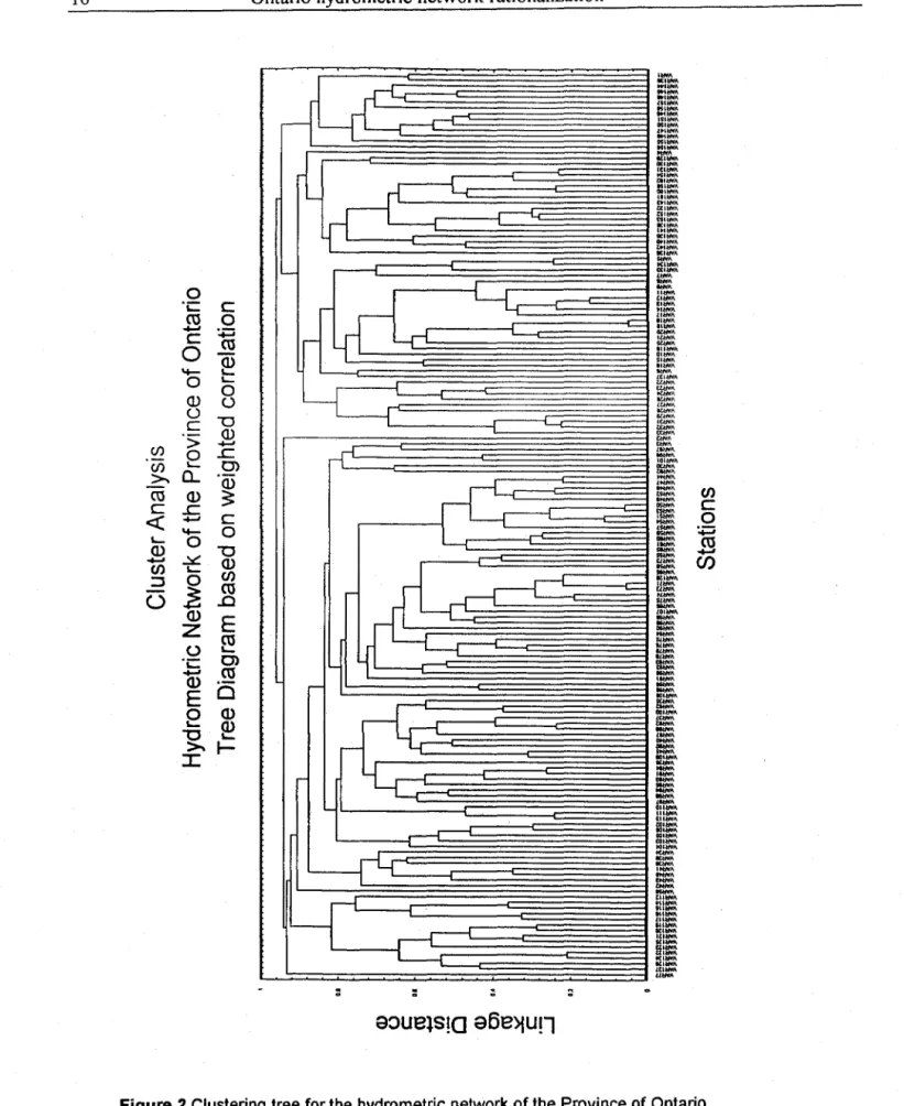
of the hydrometric network of Ontario. Figure 2 shows the tree diagram, based on weighted

correlation, for the hydrometric network of Ontario. The variables on the X-axis indicate station

numbers. 21 major groups of stations were identified on the basis of this clustering procedure. The

groups were found to correspond essentially to 21 different geographical areas of the province.

It

should be mentioned that a few stations were reclassified after the c1uster analysis to avoid

extension with auxiliary stations located unreasonably far away. A complete list of the stations of

each group is presented in Table 1. This list also indicates the identification number of each station

as they appear in the tree diagram.

4.3 Discussion of results

The result of the rationalization analysis is presented in various forms. Appendix B contains the

entire output from REDDC for each of the three variables considered (annual maximum, annual

mean, and annual minimum daily flow). The 21 groups of stations are treated one at the time.

First, the stations belonging to the particular group being examined is listed, along with

information on the length of the data records, the stations' individual contribution to

19 (denoted

"CI(act)"), the present precision of the quantile estimator, the stations' individual contribution to

Ig after n

₂

=

20 future years of full monitoring, and the precision of the quantile estimator after

n

₂

=

20 years. Then follows the results of the reduction analysis. The case of one discontinued

station is examined; the best choice is found, the program prints the results and proceeds to the

examination of the case oftwo discontinued stations, and so forth. For each eliminated station, the

program prints the name of the auxiliary station that should be used for future data extension.

It

also prints the values of n), n

₂

and n

_3,

the correlation coefficient between data at the two sites, the

station's contribution to

19 (denoted CI) after n

2 years, and the precision of the quantile estimator

after n

₂

years. The program also pro duces a matrix of group

19 values where the lines correspond

to the different groups, and the columns represent different number of removed stations. This

matrix is subsequently analysed by the program ClAT ABLE to produce the global ranking of

(23)

Cf) Cf)

~

co

c

c::(

o

ï::::

CO

....

_C

o

-

o

ID

U

C

'>

e

0...

ID

..c:

....

-

o

.:::s::.

~

_ID

Z

U

ï:::::::

....

ID

E

e

~

l

c

o

+=l

CU

~

1....

o

U

"0

ID

...

..c:

0)

"(j)

3 c

o

"0

Q)

CI)

CU

..c

E

~

0)

CU

b

Q)

~

1 -aouelS!a a6e)ju!l

CI)

c

o

+=l

J9

Cf)

(24)

4 Application

17 Table 1 Result of cluster analysis

Group 1

Group 4

Group 7

Group 10

Group 13

Group 16

Group 19

119 2KF011

102 2HOOO3

63 2GBOO7

44 2FCOOl

22 2CFOO7

5 2A0010

129 40C001

120 2LA007

103 2HOOO6

77 2GHOO3

46 2FC011

23 2CF008

6 2BA003

130 4FCool

121 2LBOO6

104 2HOOO8

80 2HAOO6

47 2FC015

24 2CF012

7 2BB003

122 2LBOO7

105 2HOOO9

81 2HA007

49 2F0002

26 20B007

133 4JC002

123 2LBOO8

106 2HOO12

83 2HBOO4

50 2FEOOS

134 4JOOOS

124 2LB017

84 2HB007

51 2FEOO9

137 4LJool

125 2LB020

85 2HB008

52 2FE011

126 2LB022

86 2HB012

53 2FE013

127 2MCool

88 2HB015

54 2FE014

128 2MC026

99 2HC03O

57 2FF007

108 2HEool

59 2GA010

60 2GA018

61 2GA038

Group 2

Group 6

Group 8

Group 11

Group 14

Group 17

Group 20

110 2HJool

36 2EC010

64 2GC002

2 2ABOO8

18 2CC005

135 4KAool

144 5POO14

111 2HK007

91 2HC009

70 2GE007

3 2AB017

19 2CC010

136 4KA002

145 5POO15

112 2HK008

92 2HC013

76 2GH002

4 2AC001

20 2COool

146 5POO17

113 2HK009

93 2HC018

78 2GHOO4

21 2COO06

147 5POO19

114 2HLOO4

94 2HC019

79 2GH011

25 2CF013

148 5P0022

115 2HLOO5

95 2HC025

118 2JC008

149 5P0023

116 2HMOO4

96 2HC027

150 5P0024

117 2HMOOS

97 2HC028

151 5P0028

98 2HC029

155 5QOOO8

101 2HC033

156 5QOO15

107 2HOO13

157 5QOO17

158 5QOO18

Group 3

Group 6

Group 9

Group 12

Group 16

Group 18

GrouQ21

34 2EC002

35 2ECOO9

55 2FF002

27 200013

8 2BFool

131 4GA002

1 2AAool

38 2E0007

37 2EOOO3

56 2FFOO4

28 200014

9 2BF002

132 4GBOO4

138 5PAOO6

39 2E0010

40 2E0014.

58 2FFOOS

29 200015

10 2BFOO4

139 5PB014

41 2FAOOl

45 2FCOO2

65 2GC010

30 200020

11 2BFOO5

140 5PB015

42 2FAOO2

62 2GA041

66 2GC018

31 2EAOOS

12 2BFOO6

141 5PB018

43 2FB007

82 2HBool

68 2G0020

32 2EA010

13 2BF007

142 5PB021

48 2FC016

87 2HB013

67 2GOO19

33 2EB013

14 2BFOOS

143 5PCOll

89 2HB018

69 2GEOOS

15 2BF009

152 5QA002

90 2HB020

71 2GG002

16 2BF012

153 5QAOO4

100 2HC031

72 2GG003

17 2CAOO2

154 5QC003

109 2HGOO1

73 2GGOOS

159 5QEOOS

74 2GGOO6

160 5QEOO9

75 2GG009

161 5QE012

162 5RCOOl

stations (details on this program is provided in the report by Rasmussen et al. (1995); a listing is

given in Appendix A). The output of the program CIATABLE is presented in Appendix C for the

three variables considered. The tables in Appendix C should be read as follows: The first column

contains the number of stations that one may wish to discontinue. The following columns give the

number of stations that should be removed from each of the 21 groups. With this information one

may retum to Appendix Band identify the stations that should be removed.

(25)

To summarize the results in a more accessible form, we have proceeded as in the project for the

Ministry ofEnvironment ofQuebec, that is, we have identified, for each of the three variables, the

first ten sites that should be removed if only statistical considerations were taken into account in

the rationalization, then the next ten stations, and so forth up to 40 stations. It is straightforward

to continue the procedure if one so wishes. Table 2 presents the result of the analysis of Appendix

Band C. The results for the minimum annual flows are not presented. Several stations have years

with zero flows or flows beIow a censoring level related to the precision of the monitoring

equipment. In general, minimum flows are much less correlated than mean annual flows or

maximum annual flows and, although record extension may be profitable from a statistical point of

view, synthetic low flow data appear to be somewhat unreliable. Therefore, we recommend

putting the main emphasis on the annual mean and annual maximum daily flows. As an additional

information, Table 2 also provides information on the correlation coefficient between the

discontinued station and its auxiliary station.

It

may be seen that the correlations generally are very

high, especially for the mean annual flow where in sorne cases it is very close to one. If mean

annual daily flow is the only variable of interest such high correlations would clearly indicate a

redundancy of information since synthetic data, obtained by record extension, would provide

almost as accurate information on the variable as actually observed data. For the mean annual

flows, the correlation for the first 40 discontinued stations are generally ab ove 0.90. Correlations

tend to be slightly smaller for annual maximum flows, but they are still quite high.

It

should be

noted that the correlation coefficient between data at a given site and data at its auxiliary station is

_.

not the only factor that affects the choice of stations to discontinue. The common period of record

is also very important, as is the Iength of the data series at the site. In fact, our definition of a

performance figure tend to favour discontinuance of stations with long records. This is because the

marginal benefit of additional data at a station with a short data record is higher than at a station

with a long record. This aspect of our performance figure may Iead to results that seem

contradictory to results from other studies. However, conflicting results are a common

phenomenon in multicriteria analyses; one will have to weight the different criteria and perform a

multicriteria analysis.

(26)

4 Application

Table 2 Result of rationalization analysis. Global ranking

of stations in network according to statistical pertinence.

Annual maximum

Annual mean

Station

rho

Station

rho

2FF002

0.96 2HB001

0.98 2GG002

0.98 2HB013

0.98 2FC001

0.93 2GB007

0.99 2FE008

0.98 2GG002

1.00

10 2FE009

0.99 2FC001

0.94 2GA010

0.93 2FE008

0.99 2EA005

0.88 2FF007

0.99 2CC005

0.98 2GA010

0.97 2BF005

0.98 2EA005

0.92 5QA002

0.92 2CC001

1.00 2LB006

0.89 2HM004

0.95 2MC001

0.94 2HC025

0.94 2HM005

0.91 2HC027

0.95 2EC002

0.72 2FC002

0.93

20 2FB007

0.79 2FF002

0.95 2FC002

0.72 2FC015

0.97 2HB001

0.84 2FE009

0.98 2FC011

0.95 2COO01

0.97 2EA010

0.89 2BF005

0.98 5PB014

0.85 5QA002

0.89 2HL005

0.81 2LA007

0.95 2HC025

0.88 2LB006

0.95 2HA007

0.81 2HL004

0.92 2G0020

0.90 2EC002

0.74

30 2GG006

0.92 2FB007

0.87 2CF007

0.91 2HC003

0.79 2COO01

0.91 2HA006

0.95 2COO06

0.93 2BF007

0.97 2BF007

0.97 2BF008

0.97 4LJ001

0.45 4JC002

0.88 2LB007

0.85 2LB007

0.93 2HOO03

0.83 2HC019

0.86 2EOO03

0.90 2HB008

0.90 2HA006

0.83 2GC018

0.97

40 2GC101

0.94 2FC011

0.95 2FC015

0.91 2GA038

0.95 2JC008

0.89 200015

0.92 2CA002

0.90 2BF001

0.89 4JC002

0.68 2BF009

0.96 4JOO05

0.85 2BB003

0.93

19

(27)

(28)

5 Conclusions

A statistical approach to hydrometric network rationalization has been applied to 162 stations in

Ontario. Based on cluster analysis, the stations were divided into 21 group with high correlations.

In the cluster analysis, both annual maximum, mean, and minimum daily flows were considered.

The 21 groups essentially corresponds to geographical regions. A few stations were manually

reclassified after the geographical regions were identified on a map. This was done to avoid record

extension with auxiliary stations that are far from the main stations. For each group, the case of

discontinuing one station, two stations, etc. was considered. At discontinued stations, a record

extension technique was used to evaluate the precision of the mean value of three hydrological

variables (annual maximum, mean, and minimum daily flows) after a certain number ofyears (20).

Adopting a global performance figure, various rationalization scenarios can be compared and the

best can be chosen. Appendix Band C provide the complete results of this analysis. In Table 2 in

Section 4 we have compiled sorne of these results into a more accessible form. Table 2 shows, in

groups of ten stations, the order in which stations should be removed from the network.

(29)

(30)

6 References

Burn,

D.H

and Goulter, I.C. An approach to the rationalization of streamflow data collection

networks, J. Hydrol., 1991, 122, 71-91.

Cochran, W.G. Sampling Techniques, John Wiley, New York, 1953.

Environment Canada, HYDAT, Version 4.94, Surface Water and Sediment Data to 1994, Atmospheric

Environment Service, CD-ROM 2245, 1996.

Matalas, N.e. and Jacobs, B. A correlation procedure for augmenting hydrologic data, U.S. Geol.

SUlV. Prof. Pap., 1964, 434-E, 7 pp.

Moran, M.A. On estimators obtained from a sample augmented by multiple regression, Water Resour.

Res., 1974, 10(1),81-85.

Ouarda, T. B.M.J., Rasmussen, P. F., and Bobée, B. On the rational reduètion ofhyrometric networks,

Proceedings of the Sixth Annual American Geophysical Union, Hydrology Days, ed.

H

J. Morel-Seytoux, Hydrology Days Publication, CA, USA, pp. 383-394, 1996.

Perron,

H,

Legendre, P. Bobée, B., and Perreault,

L. REMUS: Software for missing data recovery,

Stochastic and Statistical Methods in Hydrology and Environmental Engineering, Vol. 1, Extreme

Values: Floods and Droughts, ed K.W. Hipel, Kluwer Academic Publishers, The Netheriands, pp.

327-338, 1994.

Rasmussen, P.F, Ouarda, T.B.M.J., and Bobée, B. Rationalization of the hydrometric network for the

Province of Quebec (in French), Research Report No R-456, INRS-Eau, University of Quebec,

Quebec, 1995.

U.S. Arrny Corps of Engineers, HEC-4 monthly streamflow simulation, Generalized Computer

Program, 723-X6-L2340, Hydro!. Eng. Cent., Davis, CA., 1971

Vogel, R.M. and Stedinger, J.R. Minimum variance streamflow record augmentation procedures,

WaterResour. Res., 1985,21(5), 715-723.

(31)

(32)

APPENDIXA

(33)

function reduc(Q,names);

% function reduc(Q,names)

%

***********************************************

% 'Q' con tains the complete data set

% 'names' contains the station names

% @

Peter Rasmussen, october 1995

%

***********************************************

%---DEFINITION OF VARIOUS

CONSTANTS---n2

=

20;

%

Time horizon

T

=

100;

% Return period

zt

=

norminv(l-l/T);

%

Quanti1e in N(O,I) distribution

%---CALL SUBROUTINE "REDUCINF.m" TO GET INFORMATION ON VARIOUS

CONSTANTS---%

REDUCINF MUST CONTAIN VARIABLES ngroup, G1, .. Gn, ListStat

reducinf:

%---OPEN OUTPUT

FILE---fid = fopen('reduc.res', 'at');

fid2

=

fopen('cia.res', 'at');

%---LOG-NORMAL

TRANSFORMATION---Q(find(Q))=log(Q(find(Q))) ;

%---COMPUTE CORRELATION OF NORMAL DATA---%

disp('Computing correlation matrix')

nmat=[];rhomat=[];

for i=l:size(names,l)

end

[n rho]=statcorr(Q,i);

nmat = [nmat;n];

rhomat = [rhomat;rho];

ctisp( 'Done')

%---STORE VARIABLES FOR SUBSEQUENT

USE---Qinput=Q;

namesinput=names;

for igroup=l:ngroup

disp( ['Analyzing group' int2str(igroup)]);

fprintf(l,'*************************************\n1):

fprintf(I,'Analysis of group no. %ct in the network\n',igroup);

fprintf(l,'*************************************\n\n'};

%---GET STATIONS IN

GROUP---eval ( [' index=G' int2str (igroup) ';']);

Q - Qinput(:,index);

nstat - length(index);

names = namesinput(index, :);

rho = rhomat(index,index);

ncon = nmat(index,index);

%---GET INDEX OF STATIONS THAT WILL CERTAINLY BE

MAINTAINED---ListIndex =

[li

for i=l:size(ListStat,l)

for j=l:size(names,l)

end

if strcmp(ListStat(i,:),names(j,:))

ListIndex

=

[Listlndex j];

break

end

%---WRITE STATION INDEX, NAMES, AND OTHER

INFO---fprintf(fid, '---\n');

fprintf(fid, 'Stations in group %2d\n',igroup);

fprintf(fid, '---\n');

fprintf(fid, '%10s%5s%13s%12s%14s%10s\n', 'Name', 'N', 'CI (act) " ...

'PrQT(act) " 'CI(10a) " 'PrQT(10a)' );

LI=reshape(ListStat',I,prod(size(ListStat))) ;

for i-l:nstat

Qi

=

Q(find (Q(:, ill, i) ;

n

=

length(Qi);

Clact=std(Qi)/sqrt(n);

CIIOa-std(Qi)/sqrt(n+n2);

VarY = std(Qi)A2;

Cv - sqrt(VarY) / mean(Qi);

Zt

=

norminv(l-l/T);

VarQTact -

(1+ZtCv)A2VarY/n;

PrQTact = sqrt(VarQTact) *100;

VarQTIOa

=

(1+ZtCv)A2VarY/(n+n2);

PrQTIOa

=

sqrt(VarQTIOa) *100;

%

Variance of normal data at site i

Coefficient of variation at site

% Quantile in N(O,I) distribution

Var(QT)/QTA2 now

Var(QT)/QT

A

(34)

end

Appendix A Listing

of the

prograrns REDUC and

ClAT ABLE

str location = findstr(LI,names(i,:»;

if Ïength(str location)

&

(rem(str 10cation-l,6)==0)

fprintf (fid, '\10s*%4d%13. 5f%12 .-3f% 14 . snI O. 3f\n' , ...

names(i,:),n,CIact,PrQTact,cI10a,PrQTI0a) ;

el se

end

fprintf (tid, '\105% 5d%13. 5f% 12. 3n14. 5f% 10. 3f\n' , ...

names(i,:),n,Clact,PrQTact,CI10a,PrQTI0a

);

fprintf(fid, '\n');

fprintf(fid2,'%3d ',igroup);

for kk=O:nstat-length(ListIndex)

i f

kk==O

comb- [);

ncomb-1;

else

end

comb = cmat2(nstat,kk);

ncomb

=

size(comb,l);

Matrix of possible station combinations

Number of lines, i.e. binomial coef.

%---REMOVE ALL COMBINATIONS CONTAINING ELEMENTS FROM "ListStat"

%---THESE ARE THE STATIONS THAT WILL BE MAINTAINED WITH

CERTAINTY---for ns=1:1ength(ListIndex)

ix=(comb'-ListIndex(ns)*ones(kk,ncomb)==zeros(kk,ncomb);

if size(ix,l)==1

ix=f ind (ix) ;

else

ix=find(sum(ix) ) ;

end

if comb-=[J

If not the case of zero stations removed (kk=D)

comb (ix, :)=[);

ncomb=size(comb,l) ;

end

%---Print screen

info---fprintf(l, '\nOlimination de %d sites du r,seau',kk);

fprintf(I, '\n%d combinations are being examined\n',ncomb);

CI = 1e10D;

% Initialize variable 'bestcombvar'

for k=l:ncomb

%---GET

INDICES---jx = l:nstat;

%

Generate vector of index

if kk==O

% Index of eliminated stations

ix=[J;

else

ix

=

cOmb(k,:);

end

jx(ix)

=

[J;

% Index of remaining stations

%---FIND THE BEST EXTENSION AT EACH ELIMINATED

STATION---%

This is based on the variance of the Mean after n2 years

Vmy =

[li

Ext site=[l;

for i=ix

-minvar - 1/1ength( find(Q(:,i»);

jminvar

=

0;

Initialize variable 'minvar' which contains

the minimum extended variance at site i

%

DETERMINE BEST SITE FOR EXTENSION AT SITE l

for j=jx

nI

=

ncon(i,j);

n3

=

length(find(Q(:,i)))-nl;

%---GET

CORRELATION---if n1>=5

&

rho(i,j»O

R2 = rho (i, j) A2;

else

R2

0;

end;

Number of years of concur. data

Number of add. data at site i

%---VARIANCE OF MEAN AFTER n2 YEARS AT ELIMINATED SITE i

%---BASED ON POSSIBLE EXTENSION WITH DATA FROM SITE j

if R2* (nl-2) > (1+(n1-3)

n2n31

(n1+n2)·1 (n1+n3»)

&

n1>=5

v -

1/n1 1

(n1+n2+n3) A2

* (

(n1+n2) A2 + n1*n3

- n2(n1+n2)(R2-(1-R2)/(nl-3»);

if v<minvar

end

minvar

=

v;

jminvar = j;

If current site j yield better

extension at site i, then update

end

%

End of loop

(examination of best reconstitution at i'th Site)

(35)

end

Vmy = [Vmy std(Q(find(Q(:,i»,i»'2*minvar];

Ext site = [Ext_site jminvar];

Vector of minimum variances for the

stations removed in

combinat ion k

end

% End of loop i (evaluation of the i eliminated sites)

%---CALCULATION

or

AGGREGATED STANDARD DEVIATION IN COMBINATION

sumvar = sum(sqrt(Vmy»;

%

Agg. std at removed sites

for j=jx

% Agg. std at cont. sites

QQ

= Q(find(Q(:,j»,j);

n = length

(QQ) ;

sumvar = sumvar + std(QQ)/sqrt(n+n2);

end

\fprintf (fid, '%3d' , ix) ;

%fprintf(fid, '%10.3f\n',sumvar);

if sumvar

<

CI

:>;><

sumvar;

bestcomb - ix;

bestExt site = Ext_site;

end

% End of evaluation of combination no. k

%---OUTPUT

RESULT---i f

kk-=O

end

fprintf(fid, '\n%s%d%s%d%s\n', '* ELIMINATION DE ',kk,' SITES DU GROUPE ',igroup,' *');

fprintf (fid, '%10s%10s%6s%6s%6s%6s% 10s%10s\n', 'station', 'Aux. st.', 'nI', 'n2', 'n3', ...