An approach to improved microbial eukaryotic genome annotation

(1)

Université de Montréal

par Matthew Sarrasin

Département de Biochimie et Médicine Moléculaire, Université de Montréal, Faculté de Médicine

Mémoire présenté en vue de l’obtention du grade de M.Sc. en Bio-informatique

Décembre, 2017

(2)

ii

Ce mémoire intitulé:

An approach to improved microbial eukaryotic genome annotation

présenté par Matthew Sarrasin

a été évalué par un jury composé des personnes suivantes :

Dre Sylvie Hamel

Présidente-rapporteure

Dr B. Franz Lang

Directeur de recherche

Dre Gertraud Burger

Co-directrice de recherche

Dr Sebastian Pechmann

(3)

Résumé

Les nouvelles technologies de séquençage d’ADN ont accélérées la vitesse à laquelle les données génomiques sont générées. Par contre, une fois séquencées et assemblées, un défi continu est l'annotation structurelle précise de ces nouvelles séquences génomiques. Par le séquençage et l'assemblage du transcriptome (RNA-Seq) du même organisme, la précision de l'annotation génomique peut être améliorée, car les lectures de RNA-Seq et les transcrits assemblés fournissent des informations précises sur la structure des gènes. Plusieurs pipelines bio-informatiques actuelles incorporent des informations provenant du RNA-Seq ainsi que des données de similarité des séquences protéiques, pour automatiser l'annotation structurelle d’un génome de manière que la qualité se rapproche à celle de l'annotation par des experts. Les pipelines suivent généralement un flux de travail similaire. D'abord, les régions répétitives sont identifiées afin d'éviter de fausser les alignements de séquences et les prédictions de gènes. Deuxièmement, une base de données est construite contenant les données expérimentales telles que l’alignement des lectures de séquences, des transcrits et des protéines, ce qui informe les prédictions de gènes basées sur les Modèles de Markov Cachés généralisés. La dernière étape est de consolider les alignements de séquences et les prédictions de gènes dans un consensus de haute qualité. Or, les pipelines existants sont complexes et donc susceptibles aux biais et aux erreurs, ce qui peut empoisonner les prédictions de gènes et la construction de modèles consensus. Nous avons développé une approche améliorée pour l'annotation des génomes eucaryotes microbiens. Notre approche comprend deux aspects principaux. Le premier est axé sur la création d'un ensemble d'évidences extrinsèques le plus complet et diversifié afin de mieux informer les prédictions de gènes. Le deuxième porte sur la construction du consensus du modèle de gènes en utilisant les évidences extrinsèques et les prédictions par MMC, tel que l'influence de leurs biais potentiel soit réduite. La comparaison de notre nouvel outil avec trois pipelines populaires démontre des gains significatifs de sensibilité et de spécificité des modèles de gènes, de transcrits, d'exons et d'introns dans l’annotation structural de génomes d’eucaryotes microbiens.

Mots-clés : génome nucléaire, annotation structurale, eucaryote microbien, protistes, champignons, Saccharomyces, Neurospora, Ustilago, Plasmodium

(4)

iv

Abstract

New sequencing technologies have considerably accelerated the rate at which genomic data is being generated. One ongoing challenge is the accurate structural annotation of those novel genomes once sequenced and assembled, in particular if the organism does not have close relatives with well-annotated genomes. Whole-transcriptome sequencing (RNA-Seq) and assembly—both of which share similarities to whole-genome sequencing and assembly, respectively—have been shown to dramatically increase the accuracy of gene annotation. Read coverage, inferred splice junctions and assembled transcripts can provide valuable information about gene structure. Several annotation pipelines have been developed to automate structural annotation by incorporating information from RNA-Seq, as well as protein sequence similarity data, with the goal of reaching the accuracy of an expert curator. Annotation pipelines follow a similar workflow. The first step is to identify repetitive regions to prevent misinformed sequence alignments and gene predictions. The next step is to construct a database of evidence from experimental data such as RNA-Seq mapping and assembly, and protein sequence alignments, which are used to inform the generalised Hidden Markov Models of gene prediction software. The final step is to consolidate sequence alignments and gene predictions into a high-confidence consensus set. Thus, automated pipelines are complex, and therefore susceptible to incomplete and erroneous use of information, which can poison gene predictions and consensus model building. Here, we present an improved approach to microbial eukaryotic genome annotation. Its conception was based on identifying and mitigating potential sources of error and bias that are present in available pipelines. Our approach has two main aspects. The first is to create a more complete and diverse set of extrinsic evidence to better inform gene predictions. The second is to use extrinsic evidence in tandem with predictions such that the influence of their respective biases in the consensus gene models is reduced. We benchmarked our new tool against three known pipelines, showing significant gains in gene, transcript, exon and intron sensitivity and specificity in the genome annotation of microbial eukaryotes.

Keywords : nuclear genome, structural annotation, microbial eukaryote, protists, fungi,

(5)

List of figures

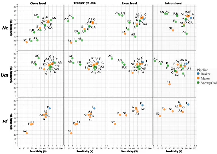
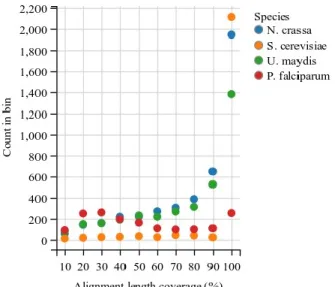
Figure 1: Overview of three commonly used protocols to prepare an RNA-Seq library. RNAs are selected and fragmented, then either synthesized to cDNAs by random priming and reverse transcription (either untagged (A) or dUTP tagged (B)), or (C) adapters are sequentially ligated followed by reverse transcription. In all cases, the final step is fragment amplification. Adapted from van Dijk et al (van Dijk, Jaszczyszyn et al. 2014). ... 26 Figure 2: Overview of the genome-guided (left) and genome-independent (right) approaches to transcriptome assembly. Reads are mapped in the genome-guided approach. Reads are then clustered per genomic loci to infer feature boundaries, which are used to construct transcript graphs. Graphs are parsed to infer possible unique paths representing putative isoforms. On the other hand, the de novo approach builds De Bruijn k-mer graphs and traverses them to infer putative transcripts. Adapted from (Garber, Grabherr et al. 2011). ... 28 Figure 3: Breakdown of the De Bruijn graph approach to de novo transcriptome assembly. a) k-mers are enumerated from sequence reads; b) De Bruijn graph is constructed from k-mers; c) paths collapsed into plausible variants; d) the graph is traversed to enumerate all variants; e) transcripts are assembled from all plausible variants. Adapted from (Martin and Wang 2011). ... 30 Figure 4: Cartoon of a HMM with three states with their respective transition and emission probabilities. For example, a simple HMM could model exons, splice junctions and introns. Adapted from (Eddy 2004). ... 33 Figure 5: Overview of the weighted consensus algorithm implemented in EVM. The top window represents transcript alignments (Nap-nr_minus_ri, AlignAssembly-r), protein alignments (Gap2-plant_gene) and gene predictions (Genewise-nr_min, Genemark, Fgenesh, GlimmerHMM) used to build consensus gene models (EVM). The Coding, Intron and Intergenic vectors (middle window) are computed to evaluate the highest scoring path through candidate exons (bottom window). See text for a more detailed description. Adapted from (Haas, Salzberg et al. 2008). ... 35 Figure 6: Specificity vs. sensitivity plots of the major steps of each pipeline at the level of genes, transcripts, exons and introns for N. crassa (Nc), U. maydis (Um) and P. falciparum (Pf). The major steps of Braker, shown in blue, include Genemark (G) and final models (F) for Maker are shown in orange. In green, the Snowyowl steps include (in order) initial Genemark predictions (G), the first round of Augustus (A), consensus predictions from Genemark and Augustus (GA), Augustus predictions with no hints (AN), coverage only (AC), coverage with splice junctions (AS), pooled models (P), representative models (R) and final models (F). ... 47 Figure 7: The number of Blast hits as a function of alignment length coverage of protein sequences against the transcriptome for the four tested species. On average, the fungi have a higher number of Blast hits, whereas P. falciparum has significantly fewer full-length hits in comparison. ... 49 Figure 8: Proposed annotation approach. RNA-Seq reads a cleaned, corrected and mapped to the genome. Mapped reads are used to guide the transcriptome assembly and to build the de novo assembly, which are combined into a non-redundant assembly. Exon-intron and CDS hints are extracted from transcript and protein sequences, respectively. Preliminary models are constructed using Genemark-ES with splice junction hints. A subset of those predictions

(9)

consistent with evidence are chosen as a training set for Augustus. Next, Augustus predictions are informed by all the extrinsic information from the assembly and alignment phase. Snap is trained on the output from Augustus, while Codingquarry is independently trained using the transcriptome assembly. Finally, a consensus set is built from the gene predictions, the transcriptome assembly and and protein alignments. ... 52

(10)

x

List of tables

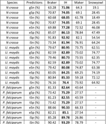
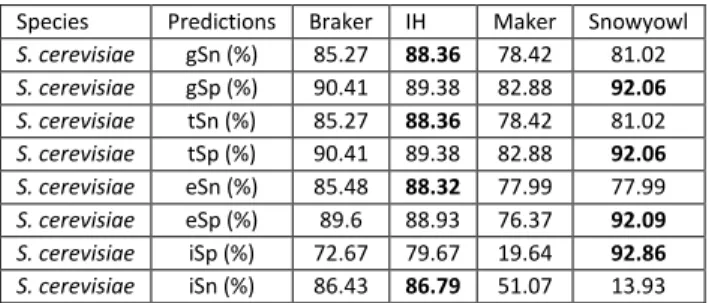
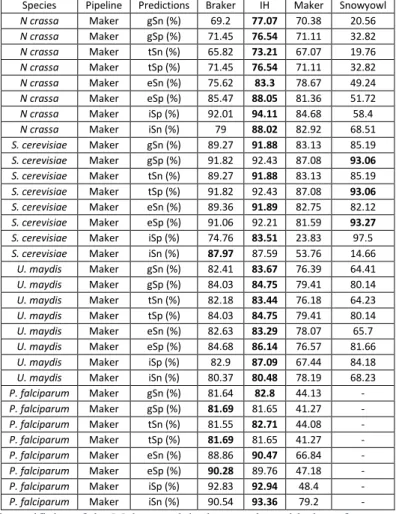
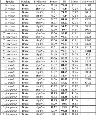
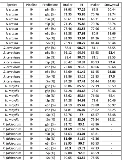
Table 1: Summary of the number (count) of protein sequence alignment falling within a relative distance of 0-0.10 (out of 0.50) out of the total number of alignments. Relative distance was computed as a function of the reference models, relative to the protein alignments, and conversely as a function of protein alignments relative to the reference models. ... 48 Table 2: Breakdown of the BUSCO results. BUSCO’s fungal and protozoa databases were searched against the fungal and protist transcriptomes, respectively. More than 200 orthologous genes are missing in the P. falciparum transcriptome assembly, whereas relatively few are missing in the fungal transcriptomes. ... 49 Table 3: Gene (gSn, gSp), transcript (tSn, tSp), exon (eSn, eSp) and intron (iSn, iSp) sensitivity and specificity of Braker, Maker, Snowyowl, and our in-house approach, with respect to the reference annotations of U. maydis, N. crassa, P. falciparum. Snowyowl was not run on P. falciparum, given that it is not a fungus (-). The highest sensitivity and specificity achieved between the pipelines, at each level, are highlighted in bold. ... 54 Table 4: Gene, transcript and exon sensitivity and specificity of Braker, Maker, our in-house approach, and SnowyOwl (fungi-only) gene models with respect to the S. cerevisiae reference. The highest sensitivity and specificity achieved between the pipelines, at each level, are highlighted in bold. The pipelines perform similarly for an intron-poor organism such as baker’s yeast. ... 55 Table 5: Summary of protein sequence alignment intervals falling within a relative distance of 00.10 (out of 0.50) for Maker and our approach tested in N. crassa with a single proteome. Relative distance was computed as a function of the reference relative to the protein alignments, and conversely as a function of protein alignments relative to the reference. ... 56 Table 6: Sensitivity and specificity of the IH, Maker and Snowyowl models with respect to the N. crassa reference annotation when the proteome of a single, evolutionarily distant relative is used as protein sequence input. The values marked with an asterisk indicate better performance with respect to Braker results of Table 3, values in bold indicate the highest specificity and sensitivity between the three listed pipelines. ... 56 Table 7: Summary of the BUSCO results on the protein sequence alignments of Maker and the proposed approach. ... 61 Table 8: Sensitivity and specificity of the Maker models that overlap with the reference, compared to the models of the other pipelines at the same genomic loci. The highest sensitivity and specificity achieved between the pipelines, at each level, are highlighted in bold. ... 61 Table 9: Sensitivity and specificity of the Snowyowl models that overlap with the reference, compared to the models of the other pipelines at the same genomic loci. The highest sensitivity and specificity achieved between the pipelines, at each level, are highlighted in bold. ... 62 Table 10: Sensitivity and specificity of the Braker models that overlap with the reference, compared to the models of the other pipelines at the same genomic loci. The highest Sensitivity and specificity achieved between the pipelines, at each level, are highlighted in bold. ... 62 Table 11: Sensitivity and specificity of the IH models that overlap with the reference, compared to the models of the other pipelines at the same genomic loci. The highest sensitivity and specificity achieved between the pipelines, at each level, are highlighted in bold. ... 63

(11)

(12)

xii

List of acronyms

A: Augustus

A#: Augustus round number

AC: Augustus with coverage information AN: Augustus with no hints

AS: Augustus with splice junction and coverage information BAM: Binary Alignment/Map

bp: Base pair

BUSCO: Benchmarking Universal Single-Copy Orthologs CDS: Coding DNA Sequence

CM: Covariance Model

EST: Expressed Sequence Tag DBN: Dynamic Bayes Network DNA: Deoxyribonucleic Acid dUTP: Deoxyuridine-triphosphatase G: Genemark

GA: Genemark-Augustus consensus predictions GFF: General Feature Format

GFF3: General Feature Format version 3 GSA: Gene-structure-aware

GTF: Gene Transfer Format HMM: Hidden Markov Model eSn: Exon Sensitivity

eSp: Exon Specificity gSn: Gene Sensitivity gSp: Gene Specificity iSn: Intron Sensitivity

(13)

iSp: Intron Specificity tSn: Transcript Sensitivity tSp: Transcript Specificity

MPSA: Multiple Protein Sequence Alignment ncRNA: non-coding Ribonucleic Acid

NGS: Next-generation Sequencing NT: Nucleotide

ORF: Open Reading Frame P: Pooled

PCR: Polymerase Chain Reaction PPX: Protein Profile Extension R: Representative

R#: Round number RD: Relative Distance RNA: Ribonucleic Acid RNA-Seq: RNA Sequencing S#: Snap round number

SAM: Sequence Alignment/Map Sn: Sensitivity

SNP: Single-Nucleotide Polymorphism Sp: Specificity

(14)

xiv

List of abbreviations

Contig: Contiguous Sequence Element Indel: Insertion/Deletion

k-mer: Subsequence of length k N. crassa: Neurospora crassa

P. falciparum: Plasmodium falciparum S. cerevisiae: Saccharomyces cerevisiae U. maydis: Ustilago maydis

(15)

(16)

xvi

Acknowledgements

The work presented here would not have been possible without the help of at least a dozen people. First, I thank my research director, Franz Lang, for providing me the opportunity to ask my own questions, to be part of something bigger, but also for providing guidance to stay on track. I also thank my research co-director, Gertraud Burger, for invaluable lessons on how to tell a compelling scientific story.

Of course, I thank all my colleagues for their contributions to this project, and for enriching my experience as a graduate student. In no particular order: Lila Salhi, Lise Forget, Simon Laurin-Lemay, Sandrine Moreira, Matus Valach, Rachid Daoud, Mohamed Aoulad-Aissa, Mohammed Hafez, Nicholas Schweiger and Jean-François Théroux.

Thanks to family and friends for supporting me and believing that I would, one day, make it through.

(17)

1. Introduction

I. Genomes across the tree of life

The genome is an organism’s hereditary basis. It is the genetic material contained in chromosomal DNA, the DNA of mitochondria and various plastids, and plasmid DNA. Viruses, albeit neither free-living nor cells, also contain genomes either in the form of DNA or RNA. As

of December 5th_{, 2017, genomes of over 33,000 species have been deposited at the National}

Center for Biotechnology Information (NCBI) (ftp.ncbi.nlm.nih.gov/genomes)–not to mention the many more that are about to become publicly available. Of the 33,000 genome sequences, a quarter are from viruses, 60% from bacteria, 4% from archaea, and 8% (i.e., 2,589) from the eukaryotic nucleus. In addition, nearly 10,000 organelle genomes are available, of which 75% are mitochondrial and 25% plastidal. Though NCBI's repository of genomic information represents only a small fraction of the tree of life, the currently available data provide a glimpse into the striking diversity in genome architecture and content.

a. Genome architecture

The spectrum of genome sizes ranges from the 2 kilobase (kb) circovirus genomes, to purportedly hundreds of Gbp of some eukaryotic nuclear genomes (Pellicer, Fay et al. 2010). Genome sizes cluster into roughly three groups (Koonin 2011). Viruses tend to have the smallest genomes on average but can reach sizes greater than those of the second group, bacteria and archaea (prokaryotes) (Philippe, Legendre et al. 2013). In turn, certain bacteria, e.g. the myxobacterium Sorangium cellulosum, possess genomes that exceeds 13 Mbp, which is larger than the nuclear genome of Saccharomyces cerevisiae for example (Belyi, Levine et al. 2010). Thus, there is considerable overlap between genome-size clusters such that sharp boundaries cannot be drawn between the three groups. However, a distinctive feature of the respective groups is the arrangement of functional and non-functional genome regions (referred to as genome architecture), as specified in the following sections (b-e).

b. Viruses

Viral genomes consist of either DNA or RNA, are linear or circular, single- or double-stranded, and may be made up of multiple discrete fragments (Dimmock, Easton et al. 2016). Among the smallest known virus genomes are those of single-stranded DNA circoviruses, which contain

(18)

two protein-coding genes in roughly 2 kb-long molecule (Belyi, Levine et al. 2010). On the other hand, the largest virus genomes are those of double-stranded DNA pandoraviruses, at around 2.5 Mb containing about 2,500 genes (Philippe, Legendre et al. 2013). Viruses with genomes made of RNA are more abundant than DNA viruses. Their genome sizes average around 10 kb and are often multipartite (Dimmock, Easton et al. 2016). Despite a significant diversity in genome layout, a common feature to all known viral genomes is the extremely high gene density such that genes often overlap (Firth and Brown 2006).

c. Prokaryotes

Although bacteria and archaea are fundamentally different from each other, they have genome features in common that distinguish them from eukaryotes. Hence, bacteria and archaea are often referred to as 'prokaryotes'. Prokaryotic genomes are composed of double-stranded DNA, typically in circular conformation, yet cases of linear chromosomes exist. Additional circular and linear, self-replicating, double-stranded DNA molecules, known as a plasmid, are most often encountered in bacteria. These extrachromosomal elements carry genes that can impart a survival advantage under specific conditions, such as synthesis of an antibiotic or protection against an antibiotic. Prokaryotes have generally a high gene density—albeit not as high as viruses—with short intergenic regions and mostly uninterrupted genes ((Rogozin, Makarova et al. 2002); but see (Lambowitz and Belfort 1993) and references therein). That being said, the defining architectural feature of prokaryotes is the operon. Operons are modules of spatially close and functionally-linked genes that are co-regulated and co-transcribed (Jacob and Monod 1961). Such co-localisation usually includes two to four genes (Salgado, Moreno-Hagelsieb et al. 2000), and sometimes dozens more, as for example genes encoding subunits of the ribosomal supercomplex (Wolf, Rogozin et al. 2001). The composition of operons is more likely to be conserved than their synteny (Tatusov, Mushegian et al. 1996).

d. Eukaryotes

The range in eukaryotic nuclear genome sizes spans several orders of magnitude. One of the smallest genomes has been observed in the unicellular parasitic eukaryote Encephalitozoon at around 2.4 Mb (Katinka, Duprat et al. 2001), whereas the largest genomes have been documented in plants. For example, the nuclear genome size of the Japanese Canopy plant Paris

japonica exceeds 120 Gb (Pellicer, Fay et al. 2010), i.e. it is more than 40 times as large as that

(19)

fungi (~1,800), animals (~400) and plants (~200). The remaining ~200 nuclear genomes come from a taxonomically broad range of less well-known and less well-studied eukaryotic groups such as Archaeplastida, Stramenopiles, Alveolata, Rhizaria, Discoba, Amoebozoa, Hacrobia, Apusozoa and Opisthokonta (Adl, Simpson et al. 2005, Hampl, Hug et al. 2009, Okamoto, Chantangsi et al. 2009). These supergroups are often referred to collectively by the catch-all term ‘protists’, referring to any eukaryotic organism that neither belongs to plants, animals nor fungi (Adl, Leander et al. 2007).

Certain trends have been observed in nuclear genome organisation, but they are not universal. The majority of nuclear genes are apparently not organised as in prokaryotes. Clusters of co-transcribed genes have been documented in nematodes (Krause and Hirsh 1987), trypanosomes (Sutton and Boothroyd 1986), euglenozoans (Tessier, Keller et al. 1991), and others (Bitar, Boroni et al. 2013), though they do not function like operons. Non-random arrangement of functionally linked genes has been found to be correlated with tandem duplications, like the ANTP-like homeobox genes in animals (Ferrier and Holland 2001). Co-expression has also been correlated with co-localisation of genes. More than 25% of yeast genes co-expressed during the mitotic cell cycle are clustered on the same chromosome (Cho, Campbell et al. 1998). In animals, however, clustering of co-expressed genes only accounts for <5% of all coding genes (Sémon and Duret 2006).

The predominant architectural genome features that set eukaryotes apart from prokaryotes is the composition, abundance and location of non-coding DNA. One particular type almost uniquely found in eukaryotes are the non-coding segments (introns) that interrupt coding segments (exons). Other forms of non-coding DNA tend to be more abundant in eukaryotes compared to prokaryotes, including repetitive regions (simple and tandem, transposable elements, duplications, pseudogenes), non-coding genes (discussed later), and other intergenic DNA. The general trend is that genomes distended with numerous long introns and other types of non-coding DNA tend to be observed in higher eukaryotes such as humans (Mattick 2001).

The number, length and composition of introns varies substantially between taxa, and even within the same genus. Some nuclear genomes can contain relatively few (<200 total) introns that are often short (<100 bp median length) as seen, for example, in S. cerevisiae

(20)

(Spingola, Grate et al. 1999), the diplomonad G. lamblia (Nixon, Wang et al. 2002) and kinetoplastids in general (e.g. T. brucei) (Muhich and Boothroyd 1988). On the opposite end of the spectrum, protein-coding genes (averaging 2 kb in length, and some exceeding 10 kb) in vertebrates have between five to eight introns (Gibbs, Weinstock et al. 2004). Despite the variability in number and length, intron positions in coding genes tend to be conserved even across large evolutionary distances. For instance, as many as 30% of introns are inserted at the same positions in orthologous genes from vertebrates and plants (Fedorov, Merican et al. 2002). The total amount of coding DNA, and the proportion of repetitive regions, non-coding genes or other types of intergenic DNA, also vary considerably. For example, around 52% of the E. cuniculi genome (Katinka, Duprat et al. 2001), and around 41% of the

Trypanosoma cruzi genome (El-Sayed, Myler et al. 2005), is non-coding DNA. Higher

eukaryotes are on the other end of the non-coding DNA abundance spectrum, where as much as 99% of the genome is non-coding DNA in humans (Lander, Linton et al. 2001) and plants (Bennetzen and Kellogg 1997). The nuclear genome of E. cuniculi contains as few as 2,000 densely packed genes, with short intergenic regions (~130bp) and with most of the non-coding DNA (~53%) found in telomeric and sub-telomeric regions (Katinka, Duprat et al. 2001). In contrast, the mean length of intergenic regions in T. cruzi is ~1,000, and a substantial amount of the repetitive regions are composed of pseudogenes (El-Sayed, Myler et al. 2005). Transposable elements make up 45% of the human genome, and even more than 50% of some plant genomes like maize ((Bennetzen and Kellogg 1997) and references therein).

e. Mitochondria and plastids

In addition to the nuclear genome, eukaryotes can also house organellar genomes. It is now widely accepted that mitochondria and plastids were once free-living bacteria (alpha-proteobacterial and cyanobacterial origins, respectively) that formed an endosymbiotic relationship with ancestral eukaryotes. The transition of the endosymbiont to an integral part of the eukaryotic cell has had a profound effect on the architecture of both the host’s and the symbiont’s genome—the latter having undergone massive genome reduction and rearrangement, even between closely related species ((Gray, Burger et al. 1999, Green 2011), and references therein). Genome conformations can be linear or circular, either in a single contiguous chromosome or spread between dozens of fragments (Gray, Burger et al. 1999, Stoebe and Kowallik 1999).

(21)

Mitochondria DNAs (mtDNAs) range from 5 kbp (Hikosaka, Watanabe et al. 2009) to 100 kbp (Burger, Gray et al. 2013) in size, with introns and intergenic regions representing anywhere from 1% to 99% of the genome ((Smith and Keeling 2015) and references therein). The highly reduced apicomplexan mitochondria (~5 kbp genomes) contain as few as three genes (cox1, cox3, cob) (Feagin, Mericle et al. 1997), whereas the mitochondria of Andalucia, the most alpha-proteobacterial-like, contains 100 genes. Of those 100 genes, at least two have been found to encode proteins (large subunit mitoribosomal protein, and a protein related to cytochrome oxidase assembly) that have, so far, only been detected in the nuclear genome of other eukaryotes (Burger, Gray et al. 2013). Gene fragmentation, manifesting in lineage-specific ways, is a peculiar feature documented in the mitochondria of green algae (Boer and Gray 1988), euglenozoans (Lukeš, Guilbride et al. 2002, Marande, Lukeš et al. 2005) and alveolates (Waller and Jackson 2009). Essentially, genes are present in multiple discrete pieces distributed across different DNA molecules. In Chlamydomonas mitochondria, for example, eight discrete fragments that encode the large subunit ribosomal RNA are present in different DNA molecules, and are post-transcriptionally spliced together (Boer and Gray 1988).

In contrast to mtDNAs, plastid DNAs (ptDNAs) can be as large as 1 Mbp in certain plants (Sloan, Alverson et al. 2012). The non-coding DNA content of ptDNAs ranges from 5-80% (Smith, Lee et al. 2010). On average, ptDNAs contain more genes than mitochondria (Barbrook, Howe et al. 2010), ranging from as few as ~20 genes in some dinoflagellates (Barbrook, Voolstra et al. 2014), up to ~250 in red algae (Janouškovec, Liu et al. 2013). Plastids can have a substantially different gene complement compared to mitochondria; the most apparent being photosynthesis-related genes in chloroplasts. Other types of plastid genomes can contain genes related to pigment synthesis and storage (chromoplasts), or monoterpene synthesis (leucoplasts) ((Wise 2007) and references therein).

II. From genome to transcriptome

The transcriptome is defined as the full range of molecules transcribed from a subset of the genetic repertoire under specific conditions in either a single cell or a (possibly heterogeneous) population of cells. Changes in conditions can rapidly induce specific readjustments in the transcriptome. Thus, the flow of information is more complex than the rather simple view of ‘from genome to transcriptome’.

(22)

a. Transcriptome composition

The different types of RNA present in the transcriptome include messenger RNA (mRNA), transfer RNA (tRNA), ribosomal RNA (rRNA), a host of mostly small non-coding RNAs (small interfering RNA (siRNA), micro RNA (miRNA), piwi-interacting RNA (piRNA), small nuclear RNA (snRNA), small nucleolar RNA (snoRNA)), long non-coding RNAs (lncRNA), and likely a range of yet-to-be characterized RNA. The respective length and abundance varies significantly between RNA classes. Small RNAs such as 5S rRNA, siRNA, miRNA, piRNA, snoRNA and tRNA, are shorter than 200 nucleotides (nt), whereas long RNAs such as mRNA, small subunit (SSU) and large subunit (LSU) rRNA and lncRNA can be as long as 17 kb (Brown, Hendrich et al. 1992). The abundance of the different RNA molecules varies by several orders of magnitude (Lodish, Berk et al. 2000). Only a small fraction of the RNA population is mRNA (~1%), while rRNA (~80%), and tRNA (15%) represent the majority, with the remainder being the various other ncRNA (Lodish, Berk et al. 2000).

b. Biological functions of transcripts

Each class of RNA molecules is linked to a specific biological function (Lodish, Berk et al. 2000). Protein synthesis involves the mRNA template to be translated, where tRNAs carry amino acids for the ribosome (composed of rRNAs and ribosomal proteins) to link together (Lodish, Berk et al. 2000). Ribosomal RNAs, in turn, are structural and enzymatically active components of ribosomes (ribozymes). Regulation in the cell can be mediated by siRNA which blocks gene expression (Hamilton and Baulcombe 1999), miRNA which blocks or accelerates degradation of mRNA (Lee, Feinbaum et al. 1993), or piRNA, which have been posited to be involved in retrotransposon silencing (Aravin, Gaidatzis et al. 2006, Girard, Sachidanandam et al. 2006).

c. Transcript processing

RNA molecules can also be modified post-transcriptionally through the processes of editing, or splicing in cis or in trans. The RNA editing machinery can substitute a nucleotide (e.g. A-to-I or C-to-U) for another, at a specific position (Benne, Van Den Burg et al. 1986). Another, but different, form of RNA processing commonly observed in eukaryotes is splicing (Lodish, Berk et al. 2000). Six snRNAs and hundreds of proteins form the small nuclear ribonucleoprotein (snRNP) complex known as the spliceosome that coordinates removal of introns from pre-mRNA (and pre-rRNA), and to join respective coding exons into a contiguous transcript. While

(23)

some interrupted protein-coding genes give rise to a single mRNA, some genes can give rise to multiple different mRNAs through the process of alternative splicing. Multiple different mRNA may be the result of exon skipping, intron retention, alternative splicing sites, alternative promoters, or a combination of any of the above (Lodish, Berk et al. 2000). The sequence of an mRNA can thus be different from an alternative mRNA originating from the same gene, which can confer an alternative function, or can change its localisation. While the most commonly observed form of splicing takes place on the same RNA molecule (in cis), trans splicing takes place between two discrete molecules.

III. Next-generation sequencing

DNA sequencing technologies have seen rapid advances along with falling costs since their inception 40 years ago—especially true for the last 15 years with the advent of next generation sequencing (NGS) (Mardis 2008, Shendure and Ji 2008, Mardis 2017). NGS offers several fundamental upgrades over previous sequencing technologies. The first major difference is in the way the library is prepared for NGS; input DNA (after fragmentation and adapter ligation) is amplified by polymerase chain reaction (PCR). Second, NGS technologies couple the sequencing and conversion of position-defined fragments to digital molecular information (Mardis 2017). The coupling of those two steps is colloquially described as “massively parallel”. The advent of NGS has opened the door to genome-wide analyses (Mardis 2017) of methylation patterns (Cokus, Feng et al. 2008), transcription factor binding sites (Sanger, Air et al. 1977, Mikkelsen, Ku et al. 2007, Cokus, Feng et al. 2008, Mardis 2017) and variants (Korbel, Urban et al. 2007). The same technology has equally been applied to deep sequencing whole transcriptomes (Mortazavi, Williams et al. 2008, Wang, Gerstein et al. 2009).

IV. Genome assembly

The genome must be reassembled from the millions of reads that are generated from widely used platforms such as Illumina (<=300 bp reads) or PacBio (<=40 kb reads). Genome assembly is a complicated procedure that is constantly evolving in response to new technologies, particularly as novel chemistries are used to increase the length of reads (Baker 2012). Effectively, the bottleneck has shifted from biochemistry to bioinformatics (Yandell and Ence 2012).

(24)

The first genomes to be assembled (Haemophilus influenzae (Fleischmann, Adams et al. 1995), baker’s yeast (Goffeau, Barrell et al. 1996) and human (Lander, Linton et al. 2001)) were done using the overlap layout consensus (OLC) method. Briefly, it can be likened to solving a jigsaw puzzle by exploiting overlap between pieces (Pop 2009). OLC assemblers (reviewed in (Miller, Koren et al. 2010)) first determine read overlaps in an all-against-all, pairwise alignment. The alignment algorithm is a heuristic search of read subsequences of length k (k-mer), otherwise known as a seed search. Next, a graph is constructed from the reads that fully or partially overlap (the jigsaw pieces that fit together) that approximates the read layout (Myers 1995). Finally, a multiple sequence alignment of the reads is computed to determine the precise layout and to resolve the consensus. An alternative was proposed by Pevzner et al. in 2001 (Pevzner, Tang et al. 2001) that can simplify assembly (particularly in repeat regions) to some extent using a De Bruijn graph. It starts by breaking reads into k-meres and building a graph of overlapping k-mers (by exactly k-1 nucleotides) and traversing the graph to reconstruct contigs, similarly to the OLC method. In both approaches, parameters are inferred from sequencing depth to help resolve repetitive regions that typically have much higher coverage than the global average (Treangen and Salzberg 2011).

a. Difficulties in genome assembly

The quality of a genome assembly is often difficult to measure given the lack of a gold standard to compare with (Salzberg, Phillippy et al. 2012). Even in long-standing assemblies such as that of the mouse nuclear genome, a number of segments are still unresolved. As much as 140 Mb (mostly from duplications) have recently been reintegrated in the mouse assembly (Church, Goodstadt et al. 2009). Issues with long repetitive regions and scaffold arrangement remain at the forefront of genome assembly, especially for libraries of shorter (20-400 bp) reads (Henson, Tischler et al. 2012, Schlebusch and Illing 2012). Difficulties can be exacerbated for certain protist genomes given that bacterial contamination—the source of food for some (Haas and Webb 1979)—is nearly impossible to avoid. No studies, to our knowledge, have yet been conducted to evaluate the extent of contamination in known protist genomes, nor to evaluate methods for removing bacterial contamination.

(25)

V. Whole transcriptome sequencing

RNA-Seq is a revolutionary procedure that, in a nutshell, provides a snapshot of all the genes expressed at a given time and condition (Mortazavi, Williams et al. 2008). It has a number of advantages over previous technologies like serial analysis of gene expression (Velculescu, Zhang et al. 1995) and tiling microarrays (Stoughton 2005). For instance, molecular information can be directly obtained from very lowly to highly expressed genes (i.e. higher dynamic range) without the need for specific restriction sites or a priori knowledge of transcripts (Parkhomchuk, Borodina et al. 2009). Thus, the full spectrum of RNAs and their absolute expression level— from mRNAs to the various non-coding RNAs (ncRNAs)—are readily available at the molecular level (Margulies, Egholm et al. 2005, Mortazavi, Williams et al. 2008, Parkhomchuk, Borodina et al. 2009). RNA-Seq has seen widespread adoption for characterising novel transcripts and quantifying expression in a population of cells (Cloonan, Forrest et al. 2008, Nagalakshmi, Wang et al. 2008, Wang, Baskerville et al. 2008, Marguerat and Bähler 2010) or, more recently, at the level of a single cell (Tang, Barbacioru et al. 2009, Islam, Kjallquist et al. 2011). Of course, depending on the type of study it is desirable to target a specific group of RNA. For example, the presence of highly expressed ribosomal RNAs could hinder signal from mRNA. Protocols have been developed to target poly-A enriched transcripts (since mRNAs typically carry an A-tail; (Cloonan, Forrest et al. 2008, Mortazavi, Williams et al. 2008), depletion kits for removing rRNA (He, Wurtzel et al. 2010), or size selection for enrichment of

(26)

small ncRNAs (reviewed in (Jacquier 2009)). Among the various experimental protocols, three are used most commonly (Figure 1).

All methods start with total RNA extraction and selection of the target class of RNA.

Branches A and B of the flowchart in Figure 1 follow similar steps to generate fragments suited for sequencing. Double-stranded cDNAs are first synthesized by reverse transcription initiated by random priming, followed by technology-specific adapter ligation for PCR amplification (van Dijk, Jaszczyszyn et al. 2014). The difference is that dUTP tagging in method B prevents sequencing of the second strand, and thus preserving the orientation of the RNA template (Parkhomchuk, Borodina et al. 2009). Preserving strand information (strand-specificity) is useful in teasing apart overlapping genes encoded on opposite strands as well as sense transcripts and (regulatory) antisense transcripts of a given gene (Normark, Bergstrom et al. 1983, Guida, Figure 1: Overview of three commonly used protocols to prepare an RNA-Seq library. RNAs are selected and

fragmented, then either synthesized to cDNAs by random priming and reverse transcription (either untagged (A) or dUTP tagged (B)), or (C) adapters are sequentially ligated followed by reverse transcription. In all cases, the final step is fragment amplification. Adapted from van Dijk et al (van Dijk, Jaszczyszyn et al. 2014).

(27)

Lindstädt et al. 2011, Wang, Jiang et al. 2014). Branch C of the flowchart describes the sequential ligation approach. It is typically employed in small RNA analyses (van Dijk, Jaszczyszyn et al. 2014).

VI. Whole-transcriptome assembly

In transcriptome assembly, similarly to genome assembly, either an OLC graph or De Bruijn graph can be applied (Florea and Salzberg 2013), but with certain adapted parametrisation. One major difference to genome assembly is that read count per gene is proportional to gene expression (Mortazavi, Williams et al. 2008). Therefore, genome assembly parametrisation is not applied to transcriptome assembly since it could lead to a loss of sensitivity in resolving transcripts whose coverage differs significantly from the average (Martin and Wang 2011). Secondly, graph parsing differs in that all transcript variants (e.g. arising from processing or alternative splicing) must be enumerated (Garber, Grabherr et al. 2011). A final consideration is whether the genome sequence is available or not; transcriptome assembly can be guided by

(28)

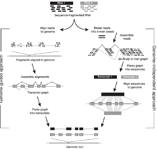
RNA-Seq reads mapped to the genome sequence, otherwise it is done de novo (Figure 2; (Martin and Wang 2011).

Figure 2: Overview of the genome-guided (left) and genome-independent (right) approaches to transcriptome

assembly. Reads are mapped in the genome-guided approach. Reads are then clustered per genomic loci to infer feature boundaries, which are used to construct transcript graphs. Graphs are parsed to infer possible unique paths representing putative isoforms. On the other hand, the de novo approach builds De Bruijn k-mer graphs and traverses them to infer putative transcripts. Adapted from (Garber, Grabherr et al. 2011).

There are advantages and disadvantages to both methods. The genome-guided (reference-based) approach requires, evidently, a high quality genome assembly. By first mapping the RNA-Seq reads to the genome, it is possible to filter out lower-quality or erroneous reads, which can reduce the complexity of assembly, and also reduce the risk of artefactual fusions (Trapnell, Williams et al. 2010). The procedure involves clustering of mapped reads at their respective genomic loci to be incorporated into a transcript graph, which is parsed to reconstruct a maximal

(29)

set of transcripts that best explain each cluster of reads (Guttman, Garber et al. 2010). The approach can have a higher sensitivity in resolving transcripts since an assembler can fill in gaps using the genomic sequence where low coverage could make reconstructing a whole transcript difficult (Guttman, Garber et al. 2010, Trapnell, Williams et al. 2010). The obvious limitation is the requirement of a genome sequence on which to map reads. The second potential drawback is that the quality of the transcriptome assembly is dependent on the quality of the genome assembly. Insertions, deletions (indels), and un-joined contigs in the genome (Salzberg and Yorke 2005), as well as extensive contaminating contigs from other organisms in the genome assembly can reduce the effectiveness of RNA-Seq read mapping, thus reducing the completeness and accuracy of the transcript assembly (Martin and Wang 2011).

(30)

In the reference-free, or de novo approach (Figure 3), a k-mer library is generated from the reads to build the transcript graph, similar to the De Bruijn-graph based genome assembly

(Grabherr, Haas et al. 2011). A unique k-mer, irrespective of coverage, represents a single node. The node is connected to another node if it overlaps by exactly k-1 nucleotides (Pevzner, Tang et al. 2001). Cases where k-mers overlap by k-2 nucleotides could indicate a single nucleotide Figure 3: Breakdown of the De Bruijn graph approach to de novo transcriptome assembly. a) k-mers are

enumerated from sequence reads; b) De Bruijn graph is constructed from k-mers; c) paths collapsed into plausible variants; d) the graph is traversed to enumerate all variants; e) transcripts are assembled from all plausible variants. Adapted from (Martin and Wang 2011).

(31)

polymorphism (SNP), sequencing error, an exon-exon (or exon-intron) junction from a variant, at which point a new branch (of length k) is created on the graph (Pevzner, Tang et al. 2001, Zerbino and Birney 2008, Martin and Wang 2011). The process is repeated on every branch, creating downstream branches if there is a k-2 overlap, until all k-mers have been accounted for. The graph is either simplified and parsed (Trapnell, Williams et al. 2010), similarly to the genome-guided approach, or the graph is directly traversed to reconstruct transcripts (Grabherr, Haas et al. 2011). An advantage is that the assembler draws from the entire pool of reads (since none have been prefiltered by mapping), which allows discovery of novel transcripts (Mortazavi, Williams et al. 2008). Uneven or missing coverage can complicate the assembly process by leading to multiple contigs although their reads were originally derived from a single transcript (Martin, Bruno et al. 2010). Increasing sequencing depth may help resolve the issue but at the same time, very high coverage (>>1,000) tends to increase the number of false positive transcripts due to base-calling errors or chimeric reads (Tarazona, Garcia-Alcalde et al. 2011).

As discussed above, both the reference-based and de novo methods each have complementary strengths and weaknesses, and are each situation-dependent. Nonetheless, if a genome assembly is available, it is advised to adopt both approaches and combine their results into a non-redundant, comprehensive assembly (Haas and Zody 2010).

VII. Annotation

The ultimate goal of genome and transcriptome assembly is to establish the genetic repertoire of an organism, through a process known as genome annotation. Genome annotation can be broken down into two major steps: 1) structural annotation, followed by 2) functional annotation (Yandell and Ence 2012). Structural annotation involves modeling various genomic features and their precise locations, namely genes, regulatory and non-coding regions. The next step is to assign to each model a biological function based on sequence similarity to known genes (Yandell and Ence 2012). Structural annotation typically consists of a suite of steps glued together into a "pipeline”. Several different pipelines exist, yet they all follow a similar workflow, which is described in the following sections.

a. Repeat masking

Generally, the first step aims at identifying repetitive regions, both tandem and dispersed repeats (Bao and Eddy 2002), and transposable elements such as long and short interspersed elements

(32)

(Bedell, Korf et al. 2000, Kapitonov and Jurka 2008). This is an important initial step since repeat regions left unmasked can misdirect Blast-like sequence alignment heuristics by anchoring seed searches in regions that yield sub-optimal alignments (Korf, Yandell et al. 2003). Unmasked repeats can also misinform gene prediction algorithms about exon-intron structure (Korf, Yandell et al. 2003, Yandell and Ence 2012).

b. Sequence alignment to generate evidence of coding gene structure

After repeat masking, it is common practice to construct a set of extrinsic evidence of gene locations and structure. Extrinsic evidence usually consists of organism-specific information (transcript assemblies) and of information from close neighbours (protein sequences), both of which can be aligned to the target organism’s genome sequence (Haas 2003, Haas, Zeng et al. 2011, Yandell and Ence 2012). A widely used heuristic tool for sequence alignment is Blast (Altschul, Gish et al. 1990), which identifies potential coding regions by exact matches of small subsequences (seed searches) and expands on matched regions using a local alignment algorithm. One considerable disadvantage in the context of structural annotation is that Blast is not capable of precisely modelling exon-intron junctions (Korf, Yandell et al. 2003). An alternative is to use spliced-sequence alignment tools, such as Exonerate or Gmap, that apply similar seed search approach as Blast but employ a computationally demanding dynamic programming algorithm around alignment gaps to identify splice junctions (Slater and Birney 2005, Wu and Watanabe 2005). Some pipelines leverage both methods: Blast is used to quickly identify putative coding regions and then intervals are "polished" with a spliced alignment tool (e.g. exonerate (Slater and Birney 2005)) to more accurately resolve start and stop codons, and splice junctions (Cantarel, Korf et al. 2008).

(33)

c. Gene prediction

Gene prediction algorithms are based on Hidden Markov Models (HMMs), but they have been generalised to include statistical properties of the genome such as G+C content, codon usage preferences and intron structure (Korf 2004). Extrinsic information extracted from RNA-Seq and sequence alignments are being used to inform both the HMMs and their generalised statistical models (Stanke, Diekhans et al. 2008). HMMs are an entirely probabilistic framework to model the most likely state (e.g. constituting an exon, intron, or intergenic region) of a given interval of a primary sequence (Rabiner 1989). The state is the "hidden" part in the Hidden Markov Model, since we do not know the underlying state a priori. The HMM consists of a transition probability (from one state to another) and an emission probability that models the composition of a state (Durbin 1998). In the context of gene prediction, a simplified HMM (Figure 4) can consist of three states: exons, splice junctions and introns, each with their own probabilities of remaining in the same state or transitioning to another (Eddy 2004). Each state

contains its own emission probabilities that could model, for example, a high chance of observing a G at an exon-intron junction, a higher chance of observing As and Ts than Gs and Cs within an intronic sequence, and a similar chance of observing any of the four nucleotides within an exon. The algorithm walks along the sequence, inferring the underlying states at each position given the previously observed sequence (a Markov chain). Many different state paths Figure 4: Cartoon of a HMM with three states with their respective transition and emission probabilities. For

(34)

potentially exist in such a probabilistic framework. For instance, referring to Figure 4, it is assumed that the first state is an exon, and the task is to determine at which locations of the sequence switches the state. The splice junction is assumed to have 95% chance of being a G, so the most likely locations of that state can be reasonably reduced to six out of twenty nucleotide positions. The algorithm explores each of those state paths in a process known as posterior decoding (Durbin 1998). The Viterbi algorithm, commonly employed in gene predictors (Lukashin and Borodovsky 1998, Stanke and Waack 2003), chooses the state with the highest log-likelihood by dynamic programming (Durbin 1998), which turns out to be position 19 in Figure 4. The inclusion of splice junctions inferred from RNA-Seq, for example, extrinsically supports a particular state path, thus increasing the accuracy of a prediction. Coverage of RNA-Seq reads can also be included to inform transitions from intergenic to initial exon states, while aligned protein sequences could support a transition to an open reading-frame state.

d. Gene model consensus

With a wealth of information from sequence alignments and HMM-based predictions about functional regions, the final step is to choose a representative model (Yandell and Ence 2012). Transcript alignments (either organism specific or from a close relative) can provide information about untranslated regions (UTRs) and coding exons, but the open reading frames (ORFs) need to be inferred (Adamidi, Wang et al. 2011). Protein sequence alignments (typically from other organisms) can fill in the gap to resolving ORFs. However, protein sequences may sometimes be insufficient. Gene predictors can give a rough look at a genome's coding content, but are strongly dependent on a high-confidence and representative training set (Burset and Guigo 1996). Therefore, pipelines have been developed to automate the process of synthesizing gene-model creation from multiple different sources to reduce the amount of manual effort required (Cantarel, Korf et al. 2008, Reid, Nicholas et al. 2014, Hoff, Lange et al. 2016, Min, Grigoriev et al. 2017). They 'combine' evidence to create a consensus using either a supervised algorithm guided by a training set (Allen and Salzberg 2005), an unsupervised algorithm using a Dynamic Bayes Network (DBN) (Liu, Mackey et al. 2008) or an algorithm based on user-defined weights per evidence source (Haas, Salzberg et al. 2008). Essentially, these pipelines each attempt to choose a model that best represents the evidence while also reducing the different types of

(35)

possible errors, such as in-frame stop codons, incorrect splice junctions, or frame shifts (Yandell and Ence 2012).

The weighted consensus process followed by EVidenceModeler (Haas, Salzberg et al. 2008) will serve as an example (Figure 5).

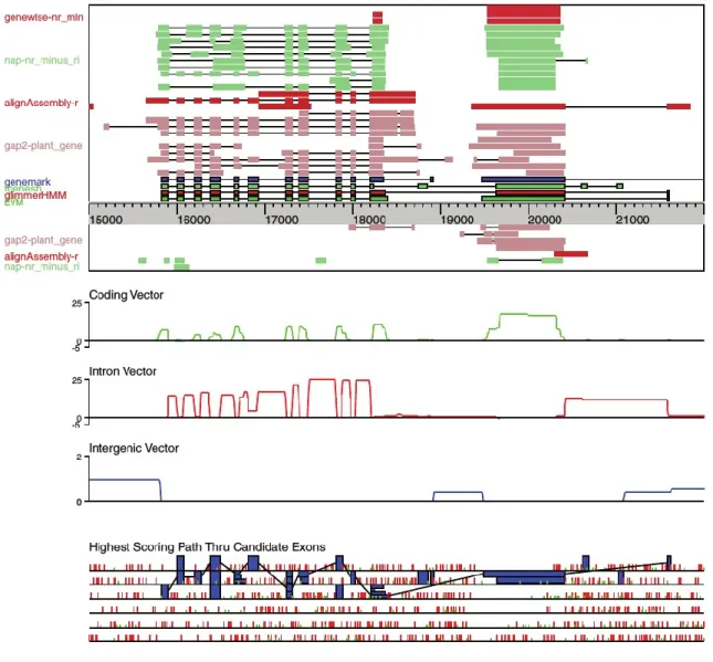
Figure 5: Overview of the weighted consensus algorithm implemented in EVM. The top window represents transcript

alignments (Nap-nr_minus_ri, AlignAssembly-r), protein alignments (Gap2-plant_gene) and gene predictions (Genewise-nr_min, Genemark, Fgenesh, GlimmerHMM) used to build consensus gene models (EVM). The Coding, Intron and Intergenic vectors (middle window) are computed to evaluate the highest scoring path through candidate exons (bottom window). See text for a more detailed description. Adapted from (Haas, Salzberg et al. 2008).

The top box is a snapshot of a 7-kb window in the rice genome with putative protein-coding regions, and several different sources of evidence to suggest its structure. Tracks labelled 'Fgenesh', 'Genemark' and 'GlimmerHMM' contain intervals inferred by the corresponding gene predictors. The Genewise and 'Nap2' tracks come from rice and non-rice protein sequence

(36)

alignments, respectively, whereas the 'AlignAssembly' and 'Nap' tracks are derived from rice and rice neighbour EST alignments, respectively. The orientation of the intervals are separated by the genomic loci axis. Position-specific score vectors are calculated for genomic features, such as coding, intron and intergenic regions, based on the evidence intervals as seen in the middle graphs of Figure 5. All possible exonic and intronic regions in the six reading frames are computed from the feature vectors, as enumerated in the bottom part of Figure 5, where green and red ticks represent start and stop codons, respectively. The vertices connecting candidate exons trace the highest scoring path computed by a dynamic programming, yielding two distinct regions in the 'EVM' track. The two regions correspond to known genes encoding the peroxisomal membrane carrier protein and 50S ribosomal protein L4, chloroplast precursor, respectively (Haas, Salzberg et al. 2008).

In contrast to the manual assignment of weights as mentioned above, the supervised training approach taken by Jigsaw infers weights from a subset of curated models, and employs a dynamic programming algorithm to resolve the highest scoring path (Allen and Salzberg 2005). Conversely, instead of relying on a training set, the DBN algorithm (employed in the Evigan pipeline) learns the parameters that best explain the evidence and then generates a consensus by computing the maximum likelihood using the Viterbi algorithm (Liu, Mackey et al. 2008), similarly to posterior decoding computed by the generalised HMMs of gene predictors. Despite the differences between the three combiners, the nematode genome assessment project (nGASP) found their performance to be similar (Coghlan, Fiedler et al. 2008). Nevertheless, the quality of consensus models may differ significantly between organisms, depending on a plethora of factors such as the available experimental data, evidence quality, evolutionary distance, among others (Yandell and Ence 2012).

e. Functional annotation

Once a complete set of organism-specific gene models have been built, the interest shifts to inferring functional information for each model. Various levels of functional information can be assigned, including secretion signals, domain content and product name, as well as broader biological implications such as pathways and processes (Frishman 2007). Pairwise similarity searches and HMM-based searches are common methods employed to elucidate function (Haas,

(37)

Zeng et al. 2011), among other specialised methods for specific tasks (e.g. localisation prediction) (Horton, Park et al. 2006).

A basic routine is to run Blast to align a query database to the target gene models whereby information associated with sequences in the query database are transferred to their respective “best hit” (i.e. best score) target sequences. Swissprot is a widely used query database, which contains many sequences with known product names, gene ontology information (molecular function, cellular localisation, biological process (Ashburner, Ball et al. 2000)), and other types of information (Boeckmann, Bairoch et al. 2003). The main advantage with Blast is that it allows for rapid transfer of information from those databases to the target sequences. In contrast to similarity algorithms, profile HMMs are an inherently probabilistic framework to detect sequence relationships with higher sensitivity. Profile HMMs are position-specific statistical models to describe the consensus of a multiple sequence alignment (i.e. the profile). The model contains information, at every given positon, to compute the true frequency of a residue relative to the observed frequency (Durbin 1998). Commonly used profile HMM databases include Pfam to search for protein domains (Bateman, Birney et al. 2002), and TIGRfam to search for protein families (Haft, Selengut et al. 2003).

VIII. Pitfalls of automated annotation

Two important challenges in every automated (structural and functional) annotation pipeline are, depending on the information they accept, (i) the introduction of systematic error due to incomplete or misleading data, (ii) errors perpetuated from incorrect comparative data and (iii) the presence of inherent biases.

a. Pitfalls in automated structural annotation

Firstly, errors can be introduced from incomplete forms of evidence. For instance, lacking RNA-Seq coverage can reduce the number of detected introns and underrepresent expressed regions as well as limit the number of successfully assembled full-length transcripts (Sims, Sudbery et al. 2014). Such errors can increase the false negative rate of gene prediction algorithms and consensus model-building tools (Yandell and Ence 2012).

Systematic biases can be introduced when inferring putative coding regions from protein sequence alignments and from gene prediction training. Since protein sequence alignment

(38)

algorithms are based on similarity searches, evolutionary distance can have varying negative effects on the diversity and completeness of information that can be leveraged. The further the distance the less useful protein sequence alignments become, which can be problematic for organisms with few characterised neighbours (Slater and Birney 2005), as is the case for most protists.

Gene prediction algorithms are also dependent on the diversity and completeness of information. A preliminary set of gene models are used to parameterise and tune generalised HMMs. Thus, a lack of preliminary models that adequately and accurately represent the full gene repertoire can bias predictions towards a particular gene structure. In turn, biased training models decrease the likelihood of detecting coding intervals (Burset and Guigo 1996).

b. Pitfalls in automated functional annotation

Systematic errors can be subtly introduced in functional annotation procedures that make use of Blast. The reason is that Blast ultimately computes a similarity score that is difficult to tie with biological relevance, especially for distantly-related sequences. As such, judging an adequate cutoff score to transfer functional information is more or less arbitrary and error prone (Galperin and Koonin 1998).

A continual challenge for databases such as Swissprot is curating data to maintain a high level of accuracy. The increasing amount of genomic data becoming available is increasingly being annotated automatically. Those models might then be used to infer functions in future projects, which could perpetuate erroneous information (Bork and Bairoch 1996). Conversely, inherent biases introduced in the structural annotation itself can have a similar effect of missing relevant information.

IX. Goals

Automated structural annotation pipelines have seen widespread adoption, yet they still cannot attain the level of accuracy of a dedicated human curator. Thus, the first goal of this project was to assess the state of current annotation pipelines by benchmarking them with “gold standard” structural genome annotations (i.e. those with considerable manual curation). The second goal was to propose a method of structural annotation to improve gene model confidence/quality, thereby reducing expert intervention.

(39)

X. Objectives

This Master research project had two objectives. The first was to identify the plausible sources of error and bias in three freely distributed, and commonly used annotation pipelines. The second objective was to develop an approach—borrowing from the same (and partially modernised) tool set of current pipelines—to specifically mitigate, if not prevent, the propagation of biases and errors. The work performed is described in the following manuscript that will be submitted for publication to Genome Biology.

(40)

2. Manuscript:

An approach to improved microbial eukaryotic genome annotation

Matthew Sarrasin, Gertraud Burger and B. Franz Lang

Target journal: Genome Biology

Contribution of authors

BFL and GB contributed to conceptual design of the approach, orchestrating the project, and writing the manuscript. MS contributed to conceptual design, implementation and validation of the study, and manuscript writing.

Keywords

Annotation, genome, eukaryote, protist, fungi, Saccharomyces, Neurospora, Ustilago,

Plasmodium

I. Abstract

Challenges in automating structural annotation of eukaryotic genomes are ever-present, particularly for eukaryote nuclear genomes without a well-annotated, closely neighbouring species. The main shortcoming of freely distributed pipelines for structural annotation come from (1) errors in incomplete input data, (2) biases in gene prediction training, and (3) inaccurate gene model consensus construction procedures. Here, we propose an improved approach that mitigates the impact of those three shortcomings. Our approach capitalizes on two main aspects; first, it leverages a more complete and diverse set of extrinsic evidence, derived from RNA-Seq and homology data, to better inform gene predictions. Second, gene models are constructed from the extrinsic evidence and gene predictions using a weighted consensus approach such that the impact of potential errors and biases is reduced. Comparative benchmarking against three widely-used pipelines shows that our approach has higher sensitivity and specificity in detecting genes, transcripts, exons and introns.

(41)

II. Background

Recent development in high-throughput whole-genome and whole-transcriptome sequencing (RNA-Seq) technology is both a boon and a burden to novel eukaryotic genome projects (Shendure and Ji 2008, Ozsolak, Platt et al. 2009, Wang, Gerstein et al. 2009, Marguerat and Bähler 2010). Although the cost of sequencing has substantially decreased, the process of finding genes and determining their exon-intron structure in a genome assembly (structural genome annotation) continues to be a challenge (Yandell and Ence 2012). Structural genome annotation is a complex multi-step process, referred to as a pipeline, to build gene models by leveraging experimental data (RNA-Seq, homology data) and predictive modeling algorithms (generalised Hidden Markov Model (HMM) gene predictions) (Yandell and Ence 2012). Several different automated pipelines have been developed to facilitate structural genome annotation by modelling the decision-making process an expert curator would follow to consolidate multiple sources of information. Among the most commonly used are Snowyowl (Reid, Nicholas et al. 2014), Maker (Cantarel, Korf et al. 2008), and Braker (Hoff, Lange et al. 2016). Snowyowl, which was specifically developed for fungal genome annotation, builds consensus gene models from concordance between gene predictions, RNA-Seq coverage and protein sequence similarity (Reid, Nicholas et al. 2014). Likewise, Maker, a generic eukaryotic annotation pipeline, extracts information about gene structure from transcript and protein sequence alignments to inform predictions and consensus gene models (Cantarel, Korf et al. 2008). In contrast, Braker was developed to only use splice junctions inferred from RNA-Seq read mapping. Though the above pipelines greatly facilitate the annotation process, some important considerations remain that can affect the quality of gene models.

One consideration is that lacking or incomplete experimental evidence can hinder gene predictions (Mathé, Sagot et al. 2002). Further, such systematic errors propagate and bias the construction of consensus gene models informed by those gene predictions and experimental evidence. Genome annotation becomes increasingly difficult for eukaryotes where relatively few of its neighbours have been characterised, and even more so for isolated, divergent taxa, as the usefulness of inferences based on sequence similarity quickly degrades (Korf 2004). Such issues can be exacerbated in genome assemblies inconspicuously contaminated with DNA from other species, e.g. bacteria being the food source of numerous unicellular eukaryotes. It becomes difficult to discern between a truly eukaryotic gene with no introns, a laterally transferred or