Solving linear systems arising from reservoirs modelling

(1)

HAL Id: tel-01984047

https://hal.inria.fr/tel-01984047v2

Submitted on 11 Jun 2020

HAL is a multi-disciplinary open access

archive for the deposit and dissemination of sci-entific research documents, whether they are pub-lished or not. The documents may come from teaching and research institutions in France or abroad, or from public or private research centers.

L’archive ouverte pluridisciplinaire HAL, est destinée au dépôt et à la diffusion de documents scientifiques de niveau recherche, publiés ou non, émanant des établissements d’enseignement et de recherche français ou étrangers, des laboratoires publics ou privés.

Hussam Al Daas

To cite this version:

Hussam Al Daas. Solving linear systems arising from reservoirs modelling. Numerical Analysis [cs.NA]. Sorbonne Université, 2018. English. �NNT : 2018SORUS329�. �tel-01984047v2�

(2)

INRIA

École doctorale École Doctorale Sciences Mathématiques de Paris Centre Unité de recherche INRIA

Thèse présentée par Hussam Al Daas

En vue de l’obtention du grade de docteur de l’Université Pierre et Marie Curie

Discipline Mathématiques appliquées Spécialité Algèbre linéaire numérique

Résolution de systèmes linéaires issus

de la modélisation des réservoirs

Thèse dirigée par Laura Grigori directrice Pascal Hénon co-directeur

(3)

(4)

INRIA

École doctorale École Doctorale Sciences Mathématiques de Paris Centre Unité de recherche INRIA

Thèse présentée par Hussam Al Daas

En vue de l’obtention du grade de docteur de l’Université Pierre et Marie Curie

Discipline Mathématiques appliquées Spécialité Algèbre linéaire numérique

Résolution de systèmes linéaires issus

de la modélisation des réservoirs

Thèse dirigée par Laura Grigori directrice Pascal Hénon co-directeur

(5)

(6)

INRIA

Doctoral School École Doctorale Sciences Mathématiques de Paris Centre University Department INRIA

Thesis defended by Hussam Al Daas

In order to become Doctor from Université Pierre et Marie Curie

Academic Field Applied Mathematics Speciality Numerical Linear Algebra

Solving linear systems arising from

reservoirs modelling

Thesis supervised by Laura Grigori Supervisor Pascal Hénon Co-Supervisor

(7)

(8)

décomposition de domaine

Keywords: krylov, block methods, inexact breakdown, deflation, recycling, domain decomposition

(9)

(10)

INRIA

2 rue Simone Iff 75012 Paris France

T +33 1 44 27 42 98 Site http://www.inria.fr/

Laboratoire Jacques-Louis Lions 4 place Jussieu

75005 Paris France

T +33 1 44 27 42 98

(11)

(12)

Solving linear systems arising from reservoirs modelling Abstract

Cette thèse présente un travail sur les méthodes itératives pour résoudre des systèmes linéaires en réduisant les communications pendant les calculs parallèles. Principalement, on est intéressé par les systèmes linéaires qui proviennent des simulations de réservoirs. Trois approches, que l’on peut considérer comme indépendantes, sont présentées. Nous considérons les systèmes linéaires non-symétriques (resp. symétriques), cela correspond au schéma explicite (resp. implicite) du problème modèle. On commence par présenter une approche qui ajoute plusieurs directions de recherche à chaque itération au lieu d’une seule direction comme dans le cas des méthodes classiques. Ensuite, on considère les stratégies de recyclage des espaces de recherche. Ces stratégies réduisent, par un facteur considérable, le nombre d’itérations global pour résoudre une séquence de systèmes linéaires. On fait un rappel des stratégies existantes et l’on en présente une nouvelle. On introduit et détaille l’implémentation parallèle de ces méthodes en utilisant un langage bas niveau. On présente des résultats numériques séquentiels et parallèles. Finalement, on considère la méthode de décomposition de domaine algébrique. Dans un environnement algébrique, on étudie le préconditionneur de Schwarz additif à deux niveaux. On fournit la forme algébrique explicite d’une classe d’espaces grossiers locaux qui bornent le conditionnement par un nombre donnéa priori.

Keywords: krylov, block methods, inexact breakdown, deflation, recycling, domain decom-position

Solving linear systems arising from reservoirs modelling Abstract

This thesis presents a work on iterative methods for solving linear systems that aim at reducing the communication in parallel computing. The main type of linear systems in which we are interested arises from a real-life reservoir simulation. Both schemes, implicit and explicit, of modelling the system are taken into account. Three approaches are studied separately. We consider non-symmetric (resp. symmetric) linear systems. This corresponds to the explicit (resp. implicit) formulation of the model problem. We start by presenting an approach that adds multiple search directions per iteration rather than one as in the classic iterative methods. Then, we discuss different strategies of recycling search subspaces. These strategies reduce the global iteration count of a considerable factor during a sequence of linear systems. We review different existing strategies and present a new one. We discuss the parallel implementation of these methods using a low-level language. Numerical experiments for both sequential and parallel implementations are presented. We also consider the algebraic domain decomposition approach. In an algebraic framework, we study the two-level additive Schwarz preconditioner. We provide the algebraic explicit form of a class of local coarse spaces that bounds the spectral condition number of the preconditioned matrix by a number pre-defined.

Keywords: krylov, block methods, inexact breakdown, deflation, recycling, domain decom-position

INRIA

(13)

(14)

INTRODUCTION

In this chapter, we give a brief introduction to the field of high performance scientific computing. We start by a short presentation of the history of computing. Then, we present the motivation for reducing communication methods. Furthermore, we present related methods that exist in the literature. Finally, we present the structure of this manuscript.

There were three necessities behind designing computers: performing arithmetical operations, reducing the time of computation, and, of course, eliminating the human liability to error. This design evolved over the history. The oldest known calculator, Abacus, goes back to as early as 2300 BC. The exact date of the invention of this tool is still unknown. During the 17thcentury many mechanical devices were invented to do arithmetical operations. One of the most famous examples is the Napier’s bones [37]. Since that time, a variety of devices have been constructed. They were not only able to do multiplication and division, but even extraction of square roots. The evolution of mechanical calculators passed by: the adding machine of Perrault (1666), of Caze (1720), and of Kummer (1847); Samuel Morland’s multiplicator (1666); Michel Rous’s instrument (1869); Léon Bollée’s multiplying and dividing machine (1893); the arithmographs of Troncet and of Clabor (beginning of 20th century); the arithmetical rods of Lucas and Genailles (beginning of 20thcentury) [37]. In the thirties of the 20th century, electromechanical computers were designed. It was Alan Turing who proposed the principles of modern computers [46]. Electronic computers have also their own evolution. It followed in somehow the electronic revolution when the transistor was invented. Arriving in 1976, the first supercomputer, called Cray-1, was installed at Los Alamos National Laboratory, USA. It used one vector processor. Six years later, the Cray X-MP was presented, the first supercomputer using shared memory parallel processors. In 1985, the first distributed memory multiprocessor supercomputer, Cray-2, saw the light. It was able to perform about 1.9 × 109floating point operations per second (1.9 Giga flops) at its peak performance. Since that time, the race competition to construct the most powerful supercomputer began. Passing by Tera flops and Peta flops, supercomputers will achieve in the coming time the Exascale (predicted by 2021).

Over the last 42 years, the transistor counts followed an exponential growth pre-dicted by Moore’s Law. Till the beginning of the 21st century, microprocessors had one

(19)

flop Bandwidth Latency

59 % Network 26% 15%

DRAM 23% 5%

Table 1 – Annual improvement of the parameters of thelatency-bandwidth model [16]. Network stands for the interconnection between processors on distributed memory architectures, DRAM is the reading access memory.

logical core. In order to have faster computing, companies had to increase the frequency. This one also increased exponentially. Consequently, the power consumption followed the exponential growth too. However, this would have become an unaffordable cost if the same strategy of increasing the frequency had been adapted. Thus, at that time, multi-core processors started to be produced. It was enough to wait two years to have a two times faster runtime of the same program on an up-to-date processor. Starting from 2005, this became different. To speedup the code, one should make it more parallel (suitable for multi-core architectures). On the other hand, distributed memory super-computers have this necessity of parallelism. Since the beginning of distributed memory supercomputers, it was noticed that moving data between processors had a large impact on the performance of the code. Two parameters play the role in moving data. The latency of the network and the bandwidth of the network. Table1presents the annual improvement of the three previous parameters. Hence, to save time, we have to decrease the movement of data. This will be referred to asreducing communication or minimizing communication in the case of asymptotic achievement of the lower bound. Furthermore,

the cost of energy ratio of moving data out of chip (DRAM, local interconnect or cross the system) to double precision floating point operation is about 100. Thus, to save energy, we have to reduce communication. To estimate the runtime of an algorithm, a performance model, called thelatency-bandwidth model, was proposed in the literature.

This model takes into account the time necessary to perform arithmetical operations, floating-point operations (flop) as well as to move data (latency and bandwidth).

In 1981 it was proved that the amount of communication necessary to perform sequential matrix-matrix multiplication has a lower bound [41]. In 2004 the proof was given for the distributed matrix-matrix multiplication [39]. Later in 2009, a generaliza-tion of these proofs was given for a wide variety of algorithms including LU factorizageneraliza-tion, Cholesky factorization, LDLT factorization, QR factorization, algorithms for eigenvalues and singular values [8]. Different algorithms were redesigned to minimize

communica-tion such as LU and QR factorizacommunica-tions [17].

Scientific simulation, cloud computing, big data, etc., are applications that need algorithms that work efficiently on heterogeneous architectures1_{. In this thesis we are}

interested in solving linear systems arising from reservoir simulations. Such systems exhibit a sparse pattern of their non-zero elements, i.e., they have a small number of non-zero elements in their coefficient matrices. This is also the case in many other applications such as other physical simulations, big data and cloud computing. The

(20)

known Gaussian elimination method (LU factorization) goes back to the 18th century. However, this method, if applied to a sparse matrix, induces a fill-in in the factors

L and U . Furthermore, the working flow of this method is hard to be parallelized.

Since they depend only on matrix-vector multiplication and dot product operations, projection iterative linear solvers appeared to be more attractive for parallelization. They are also attractive for applications in which the coefficient matrix is not assembled (e.g., due to memory limitations) and only the application of the matrix operator on a vector is possible. Krylov iterative methods are widely used iterative linear solvers. The Conjugate Gradient method [35] is a Krylov method. It is one of the top ten algorithms of the last century [75].

As we mentioned previously, we are interested in solving linear systems. More precisely, our focus is on iterative linear solvers for solving linear systems arising from reservoirs simulations. Two formulation schemes exist to model the physical problem behind the reservoirs simulations, implicit and explicit schemes [11]. The induced linear systems are non-symmetric and symmetric, respectively. Generalized Minimal Residual (GMRES) [61], Generalized Conjugate Residuals (GCR) [60], Bi-Conjugate Gradient (BiCG) [60], Bi-Conjugate Gradient stabilized (BICGSTAB) [79], and Conjugate Gradient (CG) [35] are iterative methods for solving such linear systems. These methods are based on Krylov subspace iterations. The definition of the Krylov subspace related to the matrix A ∈ Cn×nand the vector b ∈ Cnis:

Kk(A, b) = span

n

b, Ab, . . . , Ak−1bo.

One iteration of a Krylov method consists of three main operations, a vector update of the form y = αx + βy, a sparse matrix-vector multiplication SpMV, and one or multiple dot product operations. In terms of communication, the vector updates are performed locally. The sparse matrix-vector product induces point-to-point communication. However, the dot product is a global communication operation.

In order to reduce the communication, the global iteration count to reach convergence has to be reduced and/or the synchronization steps have to be hidden. To do so, different strategies were employed such as multiple search direction methods [27,9,

29, 69], hiding communication methods [24, 23], communication avoiding methods [15], deflation methods [48,20,57], and preconditioning methods [60,18,70]. Multiple search direction strategies have interesting properties. They allow to approximate the solution of multiple right-hand sides simultaneously. The operations of such methods are of a type matrix-matrix rather than a vector-vector or a matrix-vector types in single search direction methods. Thus, they can benefit from efficient Basic Linear Algebra Subprograms 3 (BLAS 3). Mostsimple (i.e. one search direction) Krylov iterative methods

have multiple search direction variants, usually referred to as block versions. Block GMRES [78], block CG [56], block BiCGSTAB [32] and other different block methods exist. Multiple direction methods can also be found in literature. Multi Preconditioned GMRES (MPGMRES) [27], Multiple Search Directions Conjugate Gradient (MSD-CG) [31], Enlarged CG (ECG), [29], and Multi Preconditioned CG (MPCG) [9,69] are variants

(21)

to enhance the convergence of Krylov methods.

Avoiding communication and hiding communication methods rely on reformulating the algorithms of thesimple Krylov methods in order to reduce synchronization steps

per iteration. The former, which is referred to as s-step methods, was firstly introduced by Chronopoulos and Gear in [15] and revisited and discussed later in [36]. The latter is referred to as pipelined methods. Pipelined CG [24] and Pipelined GMRES [23] are two examples of such methods.

Since we are interested in non-symmetric linear systems, we mostly focus on the GMRES variants. Norm-minimizing iterative Krylov methods for non-symmetric matri-ces are long recurrence methods [21]. In practice and due to memory limitations, these methods must be restarted. This leads generally to slow rate of convergence. Different methods are suggested to maintain the efficiency of the full methods (no restart variant). Deflation strategies were suggested for that aim [20,48]. Furthermore, when solving a sequence of linear systems arising from different applications (Newton’s method, Constrained Pressure Residual preconditioner [80], shift and invert eigensolvers, etc.), consecutive coefficient matrices might have a small difference or even are equal. Hence, it is important to take advantage of previously solved linear systems in order to reduce the iteration count of later linear systems. A state of the art method was proposed by Parks et al. in [57].

Preconditioning the linear systems can reduce the iteration count and make the convergence fast. Efficient preconditioners usually depend on the underlined problem which makes their implementation more difficult and non-generic. Algebraic precon-ditioners that use only the coefficient matrix exist in the literature, such as incomplete factorizations methods and algebraic domain decomposition methods [60, 13]. In-complete LU (ILU), inIn-complete Cholesky (IC) are widely known preconditioners [60]. Domain decomposition methods are usually used as preconditioners for Krylov sub-space methods. The additive Schwarz method is naturally communication-avoiding (we refer the reader to [77,18,13] for a detailed overview on domain decomposition). Hence, this method can be a good candidate for reducing the communication in the iterative solver. However, this method is not robust with respect to the number of domains2. By increasing the number of domains the condition number might deteri-orate [18]. To ensure robustness, different methods propose to add a coarse space (a

supplementary domain) in order to maintain the robustness of the method. Generalized Eigenproblem in the Overlaps, GenEO, [70], FETI-GenEO [71], the coarse space based on the local Direchlet-to-Neumann maps [51], and other coarse spaces exist in literature. These coarse spaces are available for linear systems arising from the discretization of PDEs. They are efficient and not costly to be constructed but need access to the PDEs discretization information. This makes them not fully algebraic preconditioners.

This document is organized as follows. The following Chapter1presents state of the art strategies, methods and preconditioners related to iterative linear solvers. In Chapter2we introduce the enlarged GMRES method. This method is a (block) GMRES variant based on the enlarged Krylov subspace introduced in [29]. Since this method

(22)

has a block scheme, we discuss the inexact breakdown [59] and we derive a non-costly detection test. We also discuss the deflation variant based on the strategy proposed by Erhel et al [20]. In Chapter3, we discuss the solution of a sequence of linear systems. We start by deriving the deflation of singular vectors of the iteration matrix. In [57] the authors propose two types of deflation subspaces based on the Ritz eigenvectors of the iteration matrix A or its inverse A−1. We review these deflation subspaces and we propose a deflation subspace based on the singular vectors of the iteration matrix. Due to convergence issues that might occur when the coefficient matrix changes, we propose a criterion based on the same deflation strategy to choose judiciously the deflation vectors to keep for deflating the new linear system. Afterwards, Chapter4 presents our parallel implementation of the two methods presented in Chapters 2 and3. We detail the basic linear algebra routines that we use in our implementation, the memory management, the structure of the solvers, the matrix free interface as well as the communication optimization. Numerical experiments up to 1024 × 4 cores are presented. Chapter5presents a class of efficient coarse spaces associated to the additive Schwarz preconditioner. We give an explicit algebraic formula of these spaces. These coarse spaces are efficient in the sense that they bound the condition number of the preconditioned matrix by a user pre-defined number with a minimal dimension coarse space. The coarse space introduced in [70] makes part of this class. Numerical experiments that illustrate the impact of the techniques described are discussed in each chapter.

(23)

This work led to the following Journal paper

— H. Al Daas, L. Grigori, P. Hénon, Ph. Ricoux, Enlarged GMRES for solving linear systems with one or multiple right-hand sides [5,4], Journal link, accepted in IMA Journal of Numerical Analysis, Journal link

— H. Al Daas, L. Grigori, A class of efficient locally constructed preconditioners based on coarse spaces [3] PDF, accepted in SIAM Journal on Matrix Analysis and Applications

Preprint

— H. Al Daas, L. Grigori, P. Hénon, Ph. Ricoux, Recycling of Krylov subspaces and reduction of deflation subspaces for solving sequence of linear systems [6], submitted to the ACM Transactions on Mathematical Software journal.

We note that the paper entitled "Enlarged GMRES for solving linear systems with one or multiple right-hand sides" corresponds to the Chapter2, the paper entitled "A class of efficient locally constructed preconditioners based on coarse spaces" corresponds to the Chapter5, and the preprint entitled "Recycling of Krylov subspaces and reduction of deflation subspaces for solving sequence of linear systems" corresponds to Chapters3 and a part of Chapter4.

(24)

CHAPTER 1 STATE OF THE ART

Outline of the current chapter

1.1 Othogonalization strategies 7

1.2 Krylov subspaces 9

1.2.1 Preliminaries . . . 11 1.2.2 Arnoldi’s method . . . 11

1.3 Krylov subspace methods 12

1.3.1 Classical Krylov subspace methods . . . 12 1.3.2 Variants of classical Krylov subspace methods . . . 13

1.4 Preconditioners 16

In this chapter, we present several variants of strategies and iterative linear solvers related to the Krylov subspace.

1.1 Othogonalization strategies

As we will see in the next section, the Arnoldi procedure constructs an orthogonal basis of the Krylov subspace. The Arnoldi procedure can be divided into three steps, matrix vector multiplication, orthogonalization of a vector against previous vectors, normalization of a vector. In this section, we discuss different methods to orthogonalize a set of vectors against another set of vectors as well as against each other. The Gram-Schmidt method is a well-known method to obtain an orthogonal basis vectors starting from a set of vectors. Algorithm1presents the classical Gram-Schmidt procedure. The classical Gram-Schmidt algorithm uses BLAS2 operations. However, due to finite preci-sion arithmetic, round-off errors may affect the stability of the method. Two variants

(25)

Algorithm 1Classical Gram-Schmidt procedure Require: Set of linearly independent vectors b1, . . . , bm

Ensure: v1, . . . , vman orthogonal basis vectors of span {b1, . . . , bm} 1: v1= b1/kb1k2 2: forj = 1 : m − 1 do 3: w = bj+1 4: fori = 1 : j do 5: hi= v_iHw 6: end for 7: w = w −Pj i=1vihi 8: vj+1= w/kwk2 9: end for

to the classical Gram-Schmidt exist and they are considered more numerically stable [25], namely, the classical Gram-Schmidt with reorthogonalization1, Algorithm3, and the modified Gram-Schmidt, Algorithm2, procedures. The modified Gram-Schmidt Algorithm 2Modified Gram-Schmidt procedure

Require: Set of linearly independent vectors b1, . . . , bm

Ensure: v1, . . . , vman orthogonal basis vectors of span {b1, . . . , bm} 1: v1= b1/kb1k2 2: forj = 1 : m − 1 do 3: w = bj+1 4: fori = 1 : j do 5: h = v_iHw 6: w = w − vih 7: end for 8: vj+1= w/kwk2 9: end for

procedure is less sensible to round off errors. However, it uses only BLAS1 operations. Moreover, in terms of communication, it is much more costly than the classical Gram-Schmidt. Indeed, at the jthiteration of the loop, j +1 global communication are necessary to perform the dot product operations compared to 2 global communication in the case of the classical Gram-Schmidt. The double classical Gram-Schmidt can enhance the stability of the classical Gram-Schmidt while keeping the number of global communi-cation constant at each iteration in the main loop of the procedure. Previous methods use BLAS1 and BLAS2 operations. Block variants that use BLAS3 operations exist. In the following we list the block variants of Gram-Schmidt as well as methods related to the orthogonalization of a set of small number of vectors referred to astall and skinny

matrices. The Cholesky QR algorithm [72] is an interesting candidate for the tall and

(26)

Algorithm 3Double classical Gram-Schmidt procedure Require: Set of linearly independent vectors b1, . . . , bm

Ensure: v1, . . . , vman orthogonal basis vectors of span {b1, . . . , bm} 1: v1= b1/kb1k2 2: forj = 1 : m − 1 do 3: w = bj+1 4: fori = 1 : j do 5: hi= v_iHw 6: end for 7: w = w −Pj i=1vihi 8: fori = 1 : j do 9: hi= viHw 10: end for 11: w = w −Pj i=1vihi 12: vj+1= w/kwk2 13: end for

skinny matrices. This method uses BLAS3 operations, and in terms of communication it Algorithm 4Cholesky QR algorithm

Require: Set of linearly independent vectors b1, . . . , bm

Ensure: v1, . . . , vman orthogonal basis vectors of span {b1, . . . , bm} 1: let P = (b₁, . . . , b_m)

2: compute C = PHP

3: compute Cholesky factorization of C, C = RHR

4: V = P R−1

5: set v1, . . . , vmto be the columns of V

has only one synchronization step.

The TSQR algorithm [17] is a competitive candidate for the same application. It has the same communication cost of Cholesky QR. An important advantage of using TSQR is its numerical stability comparing to the Cholesky QR. However, it requires more computational costs. We refer the reader to [17] for more details on this method.

Householder and block Householder transformation are other methods that are used to orthogonalize a set of vectors, we refer the reader to [26,64] for more details.

In the following we define the Krylov subspace related to a matrix A ∈ Cn×nand a vector b ∈ Cn

1.2 Krylov subspaces

Given a matrix A ∈ Cn×nand a vector b ∈ Cn, the Krylov subspace of dimension k related to A and b is defined as:

(27)

Algorithm 5Block classical Gram-Schmidt procedure

Require: Set of linearly independent block of vectors B1, . . . , Bm =

(B1₁, . . . , Bs1

1), . . . , (B1m, . . . , B sm m)

Ensure: V1, . . . , Vman orthogonal basis vectors of span

n (B1₁, . . . , Bs1 1), . . . , (B1m, . . . , B sm m) o 1: QR factorization of B1, B1= V1R 2: forj = 1 : m − 1 do 3: W = Bj+1 4: fori = 1 : j do 5: Hi= ViHW 6: end for 7: W = W −Pj i=1ViHi 8: QR factorization of W , W = V_j+1R 9: end for

Algorithm 6Modified block Gram-Schmidt procedure

Require: Set of linearly independent block of vectors B1, . . . , Bm =

(B1₁, . . . , Bs1

1), . . . , (B1m, . . . , B sm m)

Ensure: V1, . . . , Vman orthogonal basis vectors of span

n (B1₁, . . . , Bs1 1), . . . , (B1m, . . . , B sm m) o 1: QR factorization of B1, B1= V1R 2: forj = 1 : m − 1 do 3: W = Bj+1 4: for i = 1 : j do 5: H = V_iHW 6: W = W − ViH 7: end for 8: QR factorization of W , W = V_j+1R 9: end for

(28)

Kk(A, b) = span

n

b, Ab, . . . , Ak−1bo.

1.2.1 Preliminaries

Let A ∈ Cn×nbe a non-singular matrix and let P be a polynomial of degree k ≥ 0 with coefficients p0, . . . , pk ∈ C, i.e.,

P (X) = p0+ p1X + . . . + pkXk.

The matrix P (A) ∈ Cn×nis defined as:

P (A) = p0In+ p1A + . . . + pkAk,

where In∈ Cn×nis the identity matrix.

The minimal polynomial of A is defined as the polynomial P_A of minimal degree

kAsuch that pkA= 1 and PA(A) = 0n,n, where 0n,n∈ C

n×n_{is the zero matrix. Following}

the Cayley-Hamilton theorem, each matrix has a minimal polynomial of degree kA≤n.

Note that the matrix A−1can be expressed as a polynomial of A. Given a vector b ∈ Cn, we can also define the minimal polynomial of the dual (A, b) as the polynomial PA,bof

minimal degree kA,bsuch that pkA,b= 1 and PA,b(A)b = 0n. Note that kA,b≤kA. We refer

to kA,b as the grade of b with respect to A. An important remark is that the vector A−1b

can be expressed explicitly as a polynomial of A applied on the vector b. Proposition1 states general properties of the Krylov subspaces.

Proposition 1. The following properties hold:

— dim(K_i(A, b)) = i, for all i ≤ k_A,b

— KkA,b(A, b) = Ki+kA,b(A, b), for all i ≥ 0

— AKi(A, b)) ⊂ Ki+1(A, b), for all i ≥ 0

Since the Krylov subspace of dimension k consists of all linear combinations of the vectors b, Ab, . . . , Ak−1b, it contains all vectors of the form P (A)b where P is a polynomial

of degree k − 1. This is one reason for which these subspaces play an important role in iterative methods to solve approximately linear system of the form

Ax = b. (1.1)

Indeed, the approximate solution will be of the form P (A)b, where P is a polynomial of degree k such that P (A)b ≈ A−1b.

In the following section, we discuss the construction of basis vectors in the Krylov subspace.

1.2.2 Arnoldi’s method

Arnoldi’s method constructs a basis of the Krylov method. It was at first introduced by W. E. Arnoldi to solve eigenvalue problems [7]. The method can reduce a general

(29)

square matrix to an upper Hessenberg form via unitary transformations. Algorithm7 presents the basic algorithm of Arnoldi to construct a basis of the Krylov subspace. Two Algorithm 7Arnoldi procedure with classical Gram-Schmidt orthogonalization Require: Matrix A ∈ Cn×n, vector v1∈ Cnof norm 1, dimension of the Krylov subspace

m

Ensure: Vmbasis of the Krylov subspace Km(A, v1), HmHessenberg matrix

1: forj = 1 : m do 2: w = Avj 3: fori = 1 : j do 4: hij= vH_i w 5: end for 6: w = w −Pj i=1vihij

7: hj+1,j= kwk2, define the Hessenberg matrix Hj∈ C(j+1)×j, Hj= (hik)1≤i≤(j+1),1≤k≤j

8: ifh_j+1,j= 0 then

9: stop

10: end if

11: v_j+1= w/h_j+1,j

12: end for

possible outputs can result from Algorithm7. Either the method stops at iteration j0< m

or it performs the m iterations. The first case means that the grade of v1is equal to j0

and K_m(A, v₁) = K_j₀(A, b). Hence, V_m = {v₁, . . . , v_j₀}_{. In the second case the set of basis} vectors of Km(A, b) is Vm= {v1, . . . , vm}. Note that for j < m + 1 (j < j0+ 1 in the case where

the method stops) we have,

vj+1hj+1,j= Avj− j

X

i=1

hi,jvi,

where Vj = {v1, . . . , vj}. Or in an equivalent way,

AVj= Vj+1Hj.

1.3 Krylov subspace methods

In this section we review classical Krylov methods and several variants related to them.

1.3.1 Classical Krylov subspace methods

In this section, we review two widely known Krylov subspace methods, the Conjugate Gradient (CG) [35] and the Generalized Minimal Residual (GMRES) [61].

(30)

CG:[35] the Conjugate Gradient method is an iterative method that finds at iteration

k the approximate xk such that kx∗−x_kk_Ais minimal, where k . k_Astands for the A-norm

(A must be SPD) and x∗is the exact solution of the linear system. This method is one

of the top ten algorithms of the last century. It has a short recurrence formulation that avoids storing the Krylov subspace vectors. Algorithm8presents the simple CG method.

Algorithm 8CG

Require: Matrix A ∈ Cn×n(SPD), right-hand-side b ∈ Cn, initial guess solution x0, and

the threshold of convergence ε

Ensure: Approximate solution x such that kb − Axk₂< ε

1: r0= b − Ax0, ρ0= kr0k22, j = 1 2: while√ρj−1> εkbk2do 3: ifj == 1 then 4: p = r0 5: else 6: β = ρ_j−1/ρ_j−2, p = r + βp 7: end if 8: w = Ap 9: α = ρ_j−1/phw 10: x = x + αp 11: r = r − αw 12: ρj = krk22 13: j = j + 1 14: end while

GMRES:[61] the Generalized Minimal Residual method is an iterative method that constructs an orthonormal basis of the Krylov subspace Kk(A, b) at iteration k and finds

the approximate solution x_k such that r_k= b − Ax_k is of minimal norm (the Euclidean norm) over the Krylov subspace (A is general invertible matrix). This method has no short recurrence formulation. Thus, due to memory limitations, the method has to throw away the basis vectors of the Krylov subspace and restarts. That would lead in general to slow down the convergence. Algorithm9presents the simple GMRES method. FGMRES:[62] the Flexible GMRES is a variant of GMRES that allows to use different

preconditioners, each applied at one iteration. The disadvantage of this method is that the memory to store vectors is doubled with respect to the GMRES method.

In the following section we present a brief overview of different variants of the classical Krylov subspace methods.

1.3.2 Variants of classical Krylov subspace methods

Deflation and recycling methods

(31)

Algorithm 9GMRES

Require: Matrix A ∈ Cn×n, right-hand-sides b ∈ Cnand initial guess solution x0

Ensure: Approximate solution xm 1: r₀= b − Ax₀, β = kr₀k 2, v1= r0/β 2: forj = 1 : m do 3: w = Avj. 4: fori = 1 : j do 5: hij= vHi w. 6: end for 7: w = w −Pj i=1vihij 8: hj+1,j= kwk2 9: ifhj+1,j== 0 then 10: set m = j and go to 14 11: end if 12: vj+1= w/hj+1,j 13: end for

14: Solve the least squares problem ym= arg min y∈Cm

k_H_m_{y − βe}₁k₂_,

where Hm∈ C(m+1)×mis an upper Hessenberg matrix with non-zero coefficients (hij),

e1= (1, 0, . . . , 0)>∈ Cm+1

15: x = x₀+ V_my_m, where V_m= {v₁, . . . , v_m}

GMRES in which a fixed number of the Ritz vectors related to the matrix A−1 and the Krylov subspace are updated at the end of each cycle2. The advantage of this method with respect to the restarted GMRES is that the deflation subspace maintains the efficiency of the non-restarted (referred to as full) method. This deflation subspace has a fixed dimension. It is updated every cycle. A disadvantage of this method is that it does not allow to make benefit of the deflation subspace to solve a linear system with the same matrix and different right-hand sides.

RD-GMRES: [20] the Deflated GMRES is a variant of restarted GMRES in which a number of the Ritz vectors related to the matrix A and the Krylov subspace are computed at the end of the cycle in order to precondition the matrix A in the following cycle. The deflation subspace in this method helps to maintain the efficiency of the full GMRES when the GMRES method is restarted. Since the deflation subspace is used as a preconditioner, this method allows to solve linear systems with different right-hand sides, each at a time. The major issue of this method is that the deflation subspace dimension might increase every cycle. This would lead to memory issues. A strategy for keeping the dimension fixed can remedy this problem, however, it induces a costly computation.

GCRO-DR:[57] the Generalized Conjugate Residual with Deflated Restarting is a generalization of the GMRES-DR in which any subspace can be used in deflation. This

(32)

method is typically used for solving a sequence of linear systems. In some configurations and depending on the sequence of linear systems and the choice of the deflation subspace, the convergence might be worse than the one achieved by GMRES-DR.

Avoiding communication and hiding communication methods

s-step CG: [15,36] (later called Communication-Avoiding CG method) given a vector

b, the method suggests computing the sequence of vectors Ab, A2b, . . . , Asb by applying

the sparse matrix A s times iteratively. Since A is sparse, the communication occurs only with neighbors to compute this sequence. To orthonormalize these vectors which form the columns of a tall and skinny matrix, they use a communication-avoiding QR method such as tall and skinny QR (TSQR) [17], or Cholesky QR CholQR [72]. Theoretically, this method is equivalent to the CG method and avoids the synchronization steps during

s iterations. However, numerical stability issues appear in finite precision arithmetic

leading to convergence issues. Furthermore, combining preconditioning techniques with this method is quite difficult.

p-CG:[24] the pipelined CG is a CG variant in which additional vectors are intro-duced to the classical CG method. This variant removes the costly global communication from the standard CG algorithm by only performing a single non-blocking global com-munication per iteration. This global comcom-munication phase can be overlapped by the matrix-vector product, which typically only requires local communication. This method might suffer from numerical stability issues too.

Multiple search direction methods

The main issue of the following methods is the necessary storage of the basis vectors of the search subspace. In methods using multiple search directions to solve linear systems with one right-hand side [27,9, 29], it is in general hard to know a priori if that would reduce sufficiently the iteration count with respect to the extra computation performed.

BGMRES:[78] is a block variant of GMRES that solves a linear system with multiple right-hand sides simultaneously with the same number of synchronization steps per iteration with respect to solving one right-hand side. Furthermore, the iteration count to reach convergence is typically reduced by using a large search subspace. The amount of computation is much larger, reaching a factor s for the dot product operations per iteration, where s is the number of right-hand sides.

IBBGMRES:[59] the Inexact Breakdown Block GMRES is a block GMRES variant in which only the necessary vectors are added to the search subspace. This method can remedy the storage issues in block GMRES.

MPGMRES:[27] Multi Preconditioned GMRES is a GMRES-like method in which multiple (two or more) preconditioners are applied simultaneously, while maintaining minimal residual optimality properties. To accomplish this, a block version of Flexible GMRES is used, but instead of considering blocks starting with multiple right hand sides, the method starts with the initial residual and grows the space by applying each

(33)

of the preconditioners to all current search directions and minimizing the residual norm over the resulting larger subspace. The inconvenient part in this method is that the dimension of the subspace might increase exponentially leading to storage issues. A strategy to make the dimension of the subspace increase reasonably was suggested.

MPCG: [9] Multi Preconditioned CG is a generalization of the standard CG that uses multiple preconditioners, combining them automatically in an optimal way. The algorithm may be useful for domain decomposition techniques and other problems in which the need for more than one preconditioner arises naturally. The main issue of this method is that it loses the short recurrence formulation of the classical CG.

ECG:[29] Enlarged CG is a CG variant that consists of enlarging the Krylov subspace by a maximum given number of vectors per iteration.

1.4 Preconditioners

A preconditioner of the matrix A is an invertible matrix M such that M−1 ≈_A−1 in some sense. Given the linear system (1.1), the preconditioned system by M can be defined in different ways. The left preconditioned linear system related to (1.1) is defined as:

M−1Ax = M−1b. (1.2)

The right preconditioned linear system related to (1.1) is defined as:

AM−1x = b. (1.3)

Let x∗, x∗l, and xr∗ be the solution of (1.1), (1.2), and (1.3), respectively. The solution

of (1.1) and (1.2) are the same x∗ = xl∗, however, x∗ = M−1x∗r. If the matrix and the

preconditioner are both Hermitian Positive Definite HPD (Symmetric Positive Definite SPD in the real case), it would be more appropriate to keep the Hermitian (Symmetric) structure of the matrix in the preconditioned linear system. Hence, let M = RHR the

Cholesky decomposition of M, the symmetric preconditioned linear system is defined as:

R−HAR−1x = R−Hb. (1.4)

Krylov iterative methods might need a large number of iterations in order to con-verge. Using a preconditioner enhances the rate of convergence and make the Krylov methods more attractive. In this context, we can imagine reasonable constraints on the preconditioner such as the small cost of constructing M explicitly or implicitly and the reasonable cost of computing M−1v for any vector v. The following preconditioners are

widely used in the context of Krylov iterative methods.

Incomplete LU : [60] the general Incomplete LU factorization (ILU ) process of a sparse matrix A computes a sparse lower triangular matrix L and a sparse upper triangular matrix U so that the residual matrix R = LU − A satisfies certain constraints, such as having zero entries in some locations. Roughly, the more L and U have fill-in, the more efficient the preconditioner is (with respect to iteration count to reach

(34)

convergence). However, the preprocessing cost to compute the factors is higher when the fill-in increases.

Incomplete CholeskyIC: [60] the Incomplete Cholesky factorization is the variant of the ILU factorization for symmetric definite positive (SPD) matrices.

Block Jacobi:[60] the block Jacobi preconditioner matrix stands for a block diagonal matrix whose non-zero entry (i, j) correspond to the same (i, j) entry of the matrix A. This preconditioner is communication avoiding. Each block diagonal or multiple diagonal blocks can be associated with one processor making it able to apply it on an arbitrary vector without any necessary information available in another processor. The weak point of this preconditioner is that its efficiency is less with respect to the increase in the number of diagonal blocks.

Algebraic additive Schwarz:[13,60] the additive Schwarz is originally an iterative method to solve PDEs [77,18]. From an algebraic point of view it can be considered as a generalization of the block Jacobi methods, where the diagonal blocks might have an overlap with their neighbor diagonal blocks. The same issues and advantages of block Jacobi apply.

(35)

(36)

CHAPTER 2 ENLARGED GMRES

Outline of the current chapter

2.1 Introduction 20

2.2 Background 23

2.2.1 Notations . . . 24 2.2.2 Block Arnoldi procedure and block GMRES . . . 24 2.2.3 Block Arnoldi and exact breakdown . . . 26 2.2.4 Inexact breakdowns and subspace decomposition . . . 28

2.3 Enlarged GMRES 29

2.3.1 Enlarged GMRES algorithm . . . 31 2.4 Inexact breakdowns and eigenvalues deflation in block GMRES 33 2.4.1 Inexact breakdowns . . . 33 2.4.2 Inexact breakdowns detection . . . 35 2.4.3 Deflation of eigenvalues . . . 37 2.4.4 RD-BGMRES(m) . . . 39 2.5 CPR-EGMRES 39 2.5.1 Two-stage preconditioning . . . 42 2.6 Numerical experiments 43 2.6.1 Test problems . . . 43 2.6.2 EGMRES and RD-EGMRES . . . 49 2.6.3 CPR-EGMRES . . . 51

2.7 Conclusion 53

We propose a variant of the GMRES method for solving linear systems of equations with one or multiple right-hand sides. Our method is based on the idea of the enlarged

(37)

Krylov subspace to reduce communication. It can be interpreted as a block GMRES method. Hence, we are interested in detecting inexact breakdowns. We introduce a strategy to perform the test of detection. Furthermore, we propose a technique for deflating eigenvalues that has two benefits. The first advantage is to avoid the plateau of convergence after the end of a cycle in the restarted version. The second is to have a very fast convergence when solving the same system with different right-hand sides, each given at a different time (useful in the context of Constrained Pressure Residual preconditioner).

2.1 Introduction

In this chapter, A ∈ Cn×nis a nonsingular non-Hermitian matrix. Let the system of linear equations

AX = B, (2.1)

where X ∈ Cn×s, and B ∈ Cn×sis full rank, with s ≥ 1 the number of right-hand sides. Here, we suppose that s n. Block Krylov subspace methods are iterative schemes used to solve this type of linear systems of equations. They find a sequence of approximate solutions X1, . . . , Xj respectively in the affine spaces X0+ Kj(A, R0), where X0is the initial

guess, R₀is the corresponding initial residual and

K_j_{(A, R}₀_{) = BlockSpan}n_R₀_{, AR}₀_{, . . . , A}j−1_R₀o⊂ Cn×s is the jthblock Krylov subspace related to A and R0.

Generalized Minimal RESidual (GMRES) [61], Conjugate Gradient (CG) (Hermi-tian case) [35], Conjugate Gradient Squared (CGS) [68] and Bi-Conjugate Gradient STABilized (BiCGStab) [79] are widely used Krylov subspace methods. They were all initially introduced in the simple case s = 1. An iteration of a simple Krylov method (i.e.,

s = 1) consists of a matrix-vector multiplication (BLAS2), dot products and update of

vectors (BLAS1). In terms of high performance computing, these operations, especially the dot products, are constrained by communication (between processors or between levels of the local memory hierarchy) since the computation part becomes negligible when the number of processors increases. Thus, the block-type of Krylov methods were introduced. These schemes have three main advantages. Firstly, matrix-set-of-vectors operations are used (BLAS3). Secondly, the solution of multiple right-hand-sides are computed simultaneously. Lastly, a faster convergence can be achieved by using a larger search subspace. Generally, simple Krylov subspace methods have a block variant, (e.g., block GMRES [78], block BiCGStab [32], block CG [56]). However, one issue related to block methods is that there are few papers addressing the convergence analysis, while for the methods previously mentioned, for the case (s = 1), the literature is rich with such studies [60]. O’Leary [56], studies the convergence analysis of block conjugate gradient and presents an estimation of the error in the approximate solutions. In [66],

(38)

Simoncini and Gallopoulos generalize the theory of convergence presented in [56] to the block GMRES method. This generalization is restricted to the special case when the real part of the spectrum is positive definite.

The methods referred to as s-step methods e.g., [15, 36] are based on the idea of performing s iterations of the simple method without communication (s here is different from the number of right-hand sides that we noted above). For this, s basis vectors are computed by performing s matrix-vector multiplications, then these basis vectors are orthogonalized by using block operations. The matrix-vector products are performed without communication. This is possible due to data redundancy. Recently, the enlarged Krylov subspace approach was introduced in [29] along with a communication reducing conjugate gradient based on it. In order to enlarge the search subspace, the authors split the initial residual into multiple vectors. They construct the block Krylov subspace that is associated to the matrix A and the block of vectors that are obtained from the splitting of the initial residual. The Krylov subspace is contained in the enlarged one. Thus, in the worst cases, it converges, at least, with the necessary iterations for CG to converge. In [29], authors present promising results when the enlarged Krylov conjugate gradient is applied on linear systems that converge slowly with the simple conjugate gradient method.

Iterative methods that rely on a block version of Krylov subspace produce inexact breakdowns, which are related to a rank deficiency in the block residual or in the block of search directions, before reaching convergence [43, 22]. Different strategies

to deal with this issue are presented in the literature [54, 22, 43, 59, 33, 10, 2]. To detect inexact breakdowns in block-like GMRES, a rank test has to be done at each iteration. In [59, 10, 2], the authors propose an inexact breakdowns detection test based on SVD factorization of the block residual in the block Krylov subspace. This strategy implies the solution of the least squares problem at each iteration in order to obtain the block residual in the block Krylov subspace, then it performs its SVD factorization. The dimension of the block Krylov residual increases linearly with the number of iteration. Different strategies to update a rank-revealing factorization exist in the literature. In [74, 45], given a rank-revealing factorization of a matrix M, the authors present how to update this factorization when several lines or columns are added, by concatenation, to the matrix M. In block Krylov methods, the matrix ¯Rj (the

matrix that is factored to detect inexact breakdowns at iteration j) is different for each

j. This matrix represents the block residual by the basis vectors of the block Krylov

subspace, R_j = V_j+1R¯j. This representation changes from one iteration to another. More

precisely, the matrix ¯Rj−1 is not necessarily a sub-matrix of ¯Rj. We reformulate the

relation between Rj and the basis vectors of the block Krylov subspace by using an

update strategy of the Hessenberg matrix, see Section2. This reformulation allows to update the rank-revealing factorization and thus reduces the cost of the detection test. Solving large-scale linear systems of equations by a long-recurrence Krylov method may require restarting the method. This slows down its convergence. To avoid this issue it is common to use the deflation of eigenvalues [47, 20, 49]. Before restarting (block) GMRES, either Ritz values or harmonic Ritz values and the associated vectors

(39)

are computed to construct a deflation subspace.

In this chapter we focus on the GMRES scheme as presented in [60]. We introduce Enlarged GMRES method, referred to as EGMRES. This method is based on enlarged Krylov subspaces [29]. It is adapted for solving linear systems of equations with one or multiple right-hand sides. Anenlarging factor EF is given as a parameter. At each

iteration the dimension of the enlarged Krylov subspace increases by a number s_j be-tween 1 and s × EF, where s is the number of right-hand sides. This number sj decreases

over iterations. The dimension of the enlarged Krylov subspace stops increasing when the exact solution is contained in the enlarged Krylov subspace. The enlarged Krylov subspace contains the classical (block) Krylov subspace. EGMRES algorithm performs two global communication steps per iteration. The first corresponds to the orthogonal-ization of the new basis vectors against the previous vectors. The second is associated to the orthonormalization of the added basis vectors to the enlarged Krylov subspace. A point-to-point communication is necessary to perform the sparse matrix-matrix multi-plication (SpMM). Therefore, EGMRES and GMRES have the same number of messages per iteration. The size of the messages becomes larger in EGMRES. However, EGMRES converges faster especially on challenging linear systems, see Section2.6. Thus the number of global communication phases is reduced. In terms of arithmetics, EGMRES performs more floating point operations (flops) compared to GMRES. Nevertheless, we benefit from the efficiency of BLAS3 to perform these extra operations. In addition, this extra computation is overlapped with communication when it is possible.

The chapter is organized as follows. In Section 2.2, we give a brief discussion of existing variants of GMRES and its block version. We review exact and inexact breakdowns as introduced in [59]. We review the deflated Arnoldi procedure and the inexact breakdowns detection test that is proposed in [59].

In Section2.3, we introduce Enlarged GMRES. In Section2.4we present a strategy to reduce the size of the block basis vectors. We reformulate the detection test of inexact breakdowns presented first in [59,10]. This reformulation leads to the factorization of an s × s matrix rather than a matrix of dimension approaching js × s, where s is the number of columns of the initial block residual R0and j is the iteration number. In

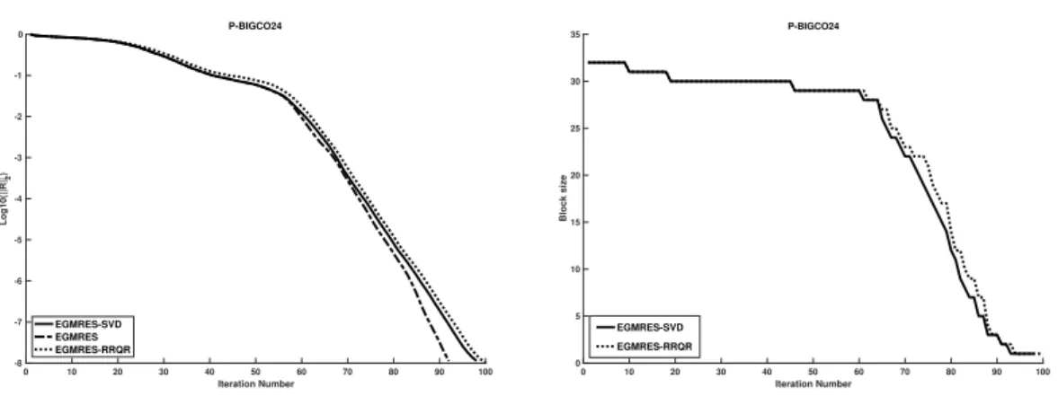
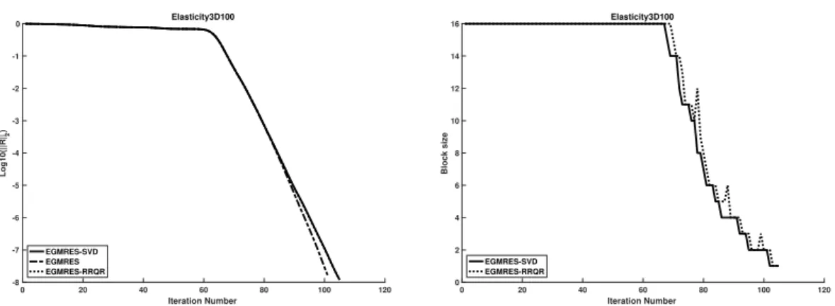
addition, we show that this s × s matrix can be computed iteratively. Furthermore, we study a new strategy based on rank-revealing QR to reduce the size of the block in BGMRES-like methods. We show that the reduced basis is sufficient to achieve the same rate of convergence as when no reduction is done. We compare our strategy on a set of matrices to the existing approach that is based on SVD [59], and we show that they have approximately the same behavior.

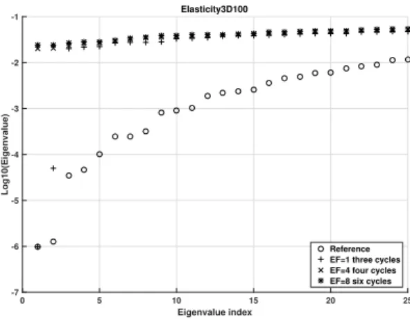
We show experimentally that the enlarged Krylov subspace method approximates better the eigenvalues of the input matrix than the classical GMRES method for the same basis size. This basis is built with a smaller number of iterations for the enlarged Krylov subspace method, hence, it costs less communication. We use this property to deflate eigenvalues between restart cycles. For this purpose, we introduce a criterion based on both the approximated eigenvalue and the norm of the residual of the associated eigenvector.

(40)

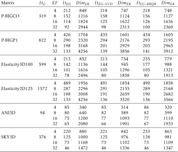
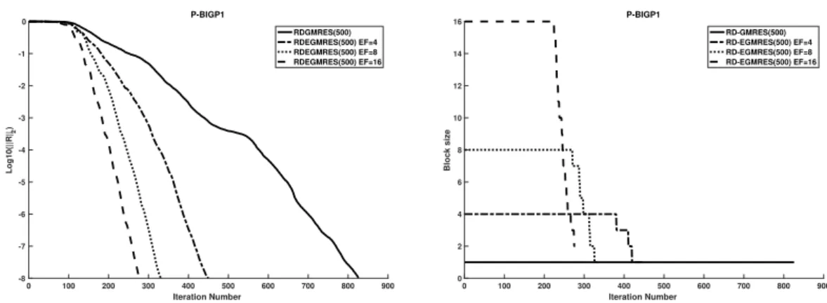
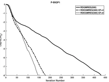
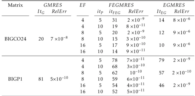
We refer to the resulting method as Restarted Deflated Enlarged GMRES or RD-EGMRES. By using RD-EGMRES, we obtain a gain of a factor up to 7 with respect to GMRES in terms of iteration count on our set of matrices. We show numerically how the enlarged Krylov subspace method better approximates the eigenvalues.

In Section2.5we adapt EGMRES to be a Constrained Pressure Residual (CPR) solver. The CPR-EGMRES is a special linear solver for saturation-pressure systems that arise from simulations of reservoirs. Since we are interested in solving linear systems arising from simulations of reservoirs, we adapt EGMRES to be used as a CPR solver, the CPR solver was introduced in [80]. Such linear systems are formed by two coupled systems. We propose to solve the global system (referred to as the second level) by using Enlarged GMRES. The first level corresponds to solving a sub-system associated with the pressure variable. This sub-system is solved at each iteration. To solve it, unlike the common choice of algebraic multigrid proposed in [63], we introduce two practical strategies based on using RD-EGMRES. Thus, by using RD-EGMRES, we benefit from the approximation of eigenvectors to solve the linear system with multiple right-hand sides that are given each one at a time. The first strategy uses a fixed number of iterations without the necessity to reach the convergence threshold. The second strategy uses the threshold of convergence as a stopping criterion. Since a Krylov iterative method is not a linear operator in general, the first strategy requires the usage of a flexible variant in the global level. Note that the second strategy can be considered as a linear operator by reason of convergence (we suppose that the convergence threshold is small enough), hence, we do not need to use the flexible variant on the second level. We compare these strategies in the numerical experiments in Section2.6. CPR-EGMRES reduces the number of iterations up to a factor of 2 compared to the ideal CPR-GMRES that solves the first level with a direct LU solver.

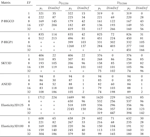
Numerical experiments are presented in Section2.6. First, we present results to show that the more we increase the enlarging factor, the faster the method converges. Furthermore, we show that reducing the basis by using the new strategy is as efficient as the approach based on SVD. We compare two thresholds for the criteria of eigenvalues deflation. This comparison is done with different maximal dimensions of the enlarged Krylov subspace. Then, we show results for linear systems of equations with multiple right-hand sides, each given at a time. This is related to the CPR preconditioner that is used later. Finally, results for linear systems of equations with multiple right-hand sides, given all at one time, are presented.

2.2 Background

In this section, we review the block GMRES method, exact breakdowns and the deflated Arnoldi procedure.

(41)

2.2.1 Notations

Matlab notations are used in a block sense: M(i, j) is the element in the block line

i and the block column j of the block matrix M. (M(i, j))i,j represents a block matrix

M whose block elements are M(i, j). k.kF represents the Frobenius norm. Let t > 0 be

the enlarging factor of the (block) Krylov subspace, and T = ts, the number of columns of the enlarged residual, where s is the number of right-hand sides. If t = 1 then, the enlarged Krylov subspace is identical to the (block) Krylov subspace. Let sj ≤s be

the number of added vectors to the basis of the block Krylov subspace K_j−1(A, R0) at

iteration j, and c_j = s − s_j. S_j =Pj

i=1si is the dimension of the block Krylov subspace

K_j_{(A, R}₀_{). We denote the cardinal by #. The identity matrix of size l is denoted by I}_l_{. The} matrix of size l × m with zero elements is denoted by 0l,m. A tilde over a matrix V , i.e.,

˜

V , means that an inexact breakdowns detection is done and this matrix is not updated

yet. A bar over a matrix V , i.e., ¯V , is the representation of V in the projection subspace

and this representation is by the constructed basis. VHrepresents the conjugate of V .

V>represents the transpose of V . R_j and RE_j are the (block) residual and the enlarged residual at the iteration j respectively. Similarly, we note X_j and X_jEthe solution and the enlarged solution. ⊕ refers to the direct sum between orthogonal subspaces. Finally, we define the following notations: ˜Vj+1∈ Cn×sj denotes the matrix whose columns are

the generated basis vectors at iteration j. Vj+1∈ Cn×sj+1 is the matrix whose columns

are effectively considered, as added vectors to the basis of K_j(A, R₀), to get K_j+1(A, R₀).

V_j _{= [V}₁_{, · · · , V}_j_{] ∈ C}n×Sj _{denotes the matrix whose columns are the basis vectors of the}

block Krylov subspace Kj(A, R0). Dj ∈ Cn×cj+1 is the matrix whose columns span the

subspace left aside in iteration j.

2.2.2 Block Arnoldi procedure and block GMRES

The block Arnoldi procedure (see Algorithm10) is the main part of the BGMRES method. It is basically the orthogonalization process applied on the new basis vectors to get an orthonormal basis for the block Krylov subspace.

(42)

Algorithm 10Block-Arnoldi (A, V1, m)

Require: Orthogonal matrix V1∈ Cn×s, matrix A ∈ Cn×n, number of iterations m.

Ensure: Orthonormal block basis vector. V_m+1_{, block Hessenberg matrix H}_m ∈ C(m+1)s×ms. 1: forj = 1 : m do 2: W = AV_j. 3: fori = 1 : j do 4: H(i, j) = V_iHW . 5: end for 6: W = W −Pj i=1ViH(i, j). 7: QR Factorization of W , W = Vj+1H(j + 1, j). 8: V_m_{= [V}₁_{, · · · , V}_m_{], V}_m+1_{= [V}_m_{, V}_m+1_{], H}_m_{= (H(i, j))}_i,j_. 9: end for

The block generalized minimal residual method (see Algorithm11), BGMRES [78], is a Krylov subspace method. It finds a sequence of approximate solutions Xj, j > 0, for

the system of linear equations AX = B. The residual norm kRjkF is minimal over the

corresponding block Krylov subspace

K_j_{(A, R}₀_{) = BlockSpan{R}₀_{, AR}₀_{, . . . , A}j−1_R₀}_. _(2.2) This method relies on building an orthonormal basis for the block Krylov subspace by using the block Arnoldi procedure. Once we build the basis, we solve a linear least squares problem in that subspace to obtain the solution.

Algorithm 11BGMRES

Require: Matrix A ∈ Cn×n, right-hand-sides B ∈ Cn×s, initial solution X0and the number

of iterations m.

Ensure: Approximate solution Xm. 1: R0= B − AX0∈ Cn×s.

2: QR Factorization of R0, R0= V1Π0.

3: Get Vm+1and Hmusing Block-Arnoldi (A, V1, m) (Algorithm10). 4: Solve the least squares problem Ym= arg min

Y ∈Cms×s

k_H_m_{Y − E}₁_Π₀k₂_, where E1= (Is, 0m,s)>∈ Cjs×s.

5: Xm= X0+ VmYm.

An algebraic relation holds at each iteration of the algorithm, AVj =P j+1

i=1ViHj(i, j).

It leads to the relation

AVj = VjHj(1 : j, 1 : j) + Vj+1Hj(j + 1, j)E >

j , (2.3)

where V_j = [V₁, · · · , V_j], and E_j = (0_s,(j−1)s, I_s)> ∈ Cjs×s_{. A detailed overview of block} Krylov methods is given in [33].

(43)

2.2.3 Block Arnoldi and exact breakdown

Definition 1. A subspace S ⊂ Cnis called A-invariant if it is invariant under the multipli-cation by A, i.e., ∀u ∈ S, Au ∈ S.

The importance of having an A-invariant subspace, for instance of dimension p, is that this subspace contains p exact eigenpairs if the matrix A is diagonalizable. In some cases, the matrix W , see (Line6, Algorithm10), is rank deficient. This occurs when an

A-invariant subspace is contained in the Krylov subspace.

Definition 2. An exact breakdown [59] is a phenomenon that occurs at the jthiteration in

the block Arnoldi procedure when the matrix W , at (Line6, Algorithm10), is rank deficient.

The order of the exact breakdown at iteration j is the integer c_j+1verifying c_j+1= s − rank(W )

where s is the rank of V1.

The following lemma is the GMRES case of [60, Proposition 6.1, p. 158]. It illustrates the importance of the breakdown in GMRES, we give its proof for completeness. Lemma 1. In GMRES, when a breakdown occurs during an iteration j, the Krylov subspace

K_j_{(A, R}₀_{) = Span{V}₁_{, · · · , V}_j}

is an A-invariant subspace.

Proof. A breakdown in GMRES occurs during the iteration j when Hj(j + 1, j) = 0. Thus,

immediately from relation (2.3), we get AVj= VjHj(1 : j, 1 : j). It yields that the subspace

Span{V₁, · · · , V_j}_{is A-invariant.}

However, in general, for the block Arnoldi procedure, an exact breakdown does not mean that there is an A-invariant subspace. For example, starting the algorithm with the initial block (u, Au), for any u ∈ Cn, yields an exact breakdown in the first iteration. Nevertheless, the obtained subspace is not necessarily A-invariant. We recall several equivalent conditions related to the exact breakdown in Theorem1. For the details and the proof see [59]. Let cj+1denote the rank deficiency of W (Line6, Algorithm10), i.e.,

cj+1= s − rank(W ), where s is the rank of V1.

Theorem 1. In the block GMRES algorithm, let X be the exact solution and R_j be the residual at iteration j. The conditions below are equivalent:

1. An exact breakdown of order cj+1at iteration j occurs.

2. dim{Range(V1) ∩ AKj(A, R0)} = cj+1.

3. rank(R_j) = s − c_j+1.

4. dim{Range(X) ∩ Kj(A, R0)} = cj+1.

(44)

As our method is based on the enlarged Krylov subspace, it naturally inherits a block version of GMRES. In the next section, we review the theory of block GMRES method with deflation at each iteration (referred to as IBBGMRES-R) proposed by Robbé and Sadkane [59]. This method was then reformulated in a different way by Calandra et

al. [10] (referred to as BFGMRES-S). Deflated Arnoldi relation

Here, we review the derivation of the modified algebraic relations of the Arnoldi procedure, presented in e.g. [59, 10]. We follow the presentation in [10]. We recall that Vj+1∈ Cn×sj+1 is the matrix formed by the columns considered to be useful and

thus, added to the basis Vj of the block Krylov subspace. Dj ∈ Cn×cj+1 is the matrix

whose columns span the useless subspace. The range of Dj is referred to as the deflated

subspace. The decomposition of the range of the matrix [ ˜Vj+1, Dj−1] into two subspaces

is

Range([ ˜Vj+1, Dj−1]) = Range(Vj+1) ⊕ Range(Dj), (2.4)

with [Vj+1, Dj]H[Vj+1, Dj] = Is. The sj+1-dimension subspace, spanned by the columns

of Vj+1, is added to the block Krylov subspace. The other cj+1-dimension subspace,

spanned by Dj, is left aside. At the end of iteration j, we want the following relation to

hold

AVj= [Vj+1, Dj]Hj, (2.5)

where the columns of Dj represent a basis of the deflated subspace after j iterations. The

columns of Vj+1, stand for a basis for the block Krylov subspace Kj+1. We assume that

this relation holds at the end of iteration j − 1. Thus,

AV_j−1= [V_j, D_j−1]H_j−1. (2.6) Let us study the iteration j. First, we multiply A by Vj. Then, we orthogonalize against

V_j _{and against D}_j−1_{. A QR factorization of the result leads us to ˜}_V_j+1_{. In matrix form} that could be written in the following equation,

AVj = [Vj, Dj−1, ˜Vj+1] ˜Hj. (2.7)

˜

Hj has the form

˜

H_j = Hj−1 Nj

0sj,Sj−1 Mj

!

(2.8) where Nj = [Vj, Dj−1]HAVj ∈ C(Sj−1+s)×sj and (AVj−[Vj, Dj−1]Nj) = ˜Vj+1Mj is the QR

factorization. To transform the relation (2.7) to the form in (2.5), let Q_j+1∈ Cs×s _{be a} unitary matrix such that

[Dj−1, ˜Vj+1]Qj+1= [Vj+1, Dj], (2.9)

then, we have