En vue de l’obtention du
DOCTORAT DE L’UNIVERSITÉ DE TOULOUSE
Délivré par l’Université Toulouse III – Paul Sabatier Discipline ou spécialité : Physique de la matière
Présentée et soutenue par Arunangshu Debnath Le 26 Septembre 2013
Titre : Dynamics and Control of open quantum systems: Applications to exciton dynamics in quantum dots and vibrational dynamics in carboxyhemoglobin
JURY
Prof. C. Meier LCAR, Toulouse Directeur de thèse Prof. M. Desouter-Lecomte LCP, Paris Examinateur Prof. V. Engel Universitat Wurzburg Examinateur Prof. N. Guihèry LCPQ, Toulouse Présidente du jury
Prof. S. Guèrin ICB, Bourgogne Rapporteur
Prof. C. Koch Universitat Kassel Rapporteur
Dr. T. Amand LPCNO, Toulouse Examinateur
Dr. C. Falvo ISMO Paris Examinateur
Dynamics and Control of Open Quantum Systems: Applications
to Exciton Dynamics in Quantum Dots & Vibrational Dynamics
in Carboxyhemoglobin
Dissertation
for partial fulfillment of Doctoral degree Universit´e Toulouse III - Paul Sabatier
Arunangshu Debnath
Burdwan, IndiaList of publications
Parts of this thesis have been published or submitted for publication in the following articles: • A. Debnath, C. Meier, B. Chatel, and T. Amand, Chirped laser excitation of quantum dot
excitons coupled to a phonon bath, Physical Review B 86, 161304 (R) (2012).
• C. Falvo, A. Debnath, C. Meier, Vibrational ladder climbing in carboxy-hemoglobin: Effects of the protein environment, The Journal of Chemical Physics 138, 14 (2013).
• A. Debnath, C. Meier, B. Chatel, and T. Amand, High fidelity biexciton generation in quantum dots by chirped laser pulses, submitted to: Physical Review B: 88, 201305 (R) (2013), Editor’s suggestions.
• A. Debnath, C. Falvo, C. Meier, State selective excitation of the CO stretch in carboxy-hemoglobin by mid-IR laser pulse shaping: a theoretical analysis,The Journal of Physical Chemistry A, Article ASAP (2013).
Contents
1 Introduction 1
2 Quantum dot: Basics 7
2.1 Introduction. . . 7
2.1.1 Quantum dot . . . 7
2.1.2 Quantum dot-Laser Interaction . . . 10
2.1.3 Phonon . . . 11
2.1.4 Exciton-phonon interaction . . . 13
2.2 Notion of Open quantum system . . . 15
2.3 The microscopic Hamiltonian . . . 15
3 Non-Markovian dynamics in quantum dots : Formalisms 17 3.1 Introduction. . . 17
3.2 Generalized master equation. . . 17
3.2.1 Projector operator formalism . . . 17
3.2.2 Context of the problem . . . 18
3.2.3 Evaluation of Memory Kernel . . . 19
3.2.4 Bath correlation function . . . 19
3.2.5 Parametrization of bath spectral density . . . 21
3.2.6 Auxiliary density matrix method . . . 22
3.3 Appendix . . . 23
3.3.1 Simplification of effective Liouvilian term . . . 23
3.3.2 Simplification of memory kernel term . . . 23
3.3.3 Bath correlation function . . . 25
3.3.4 Bath spectral density - from k space to energy space . . . 26
3.3.5 Quantum dot parameters . . . 26
4 Aspects of adiabatic population transfer I: Robust exciton generation 27 4.1 Introduction. . . 27
4.2 Dressed State Description . . . 27
4.2.1 Interaction representation and Rotating wave approximation(RWA) . . . 28
Contents
4.4 Analytical Treatment. . . 30
4.4.1 Markovian master equation in dressed basis . . . 30
4.4.2 Adiabatic Master Equation in Bloch vector representation . . . 32
4.5 Discussions . . . 35
4.5.1 Comparative assessments . . . 35
4.5.2 Prescriptions . . . 37
4.6 Remarks . . . 40
4.7 Appendix: . . . 40
4.7.1 Matrix Exponentiation of SU(2) . . . 40
4.7.2 Evaluation of dissipative kernel . . . 41
5 Aspects of adiabatic population transfer II: Robust biexciton generation 43 5.1 Introduction. . . 43
5.2 Dressed state description. . . 43
5.2.1 Interaction representation and Rotating wave approximation (RWA) . . . 44
5.3 Numerical treatment . . . 45
5.4 Analytical treatment . . . 45
5.4.1 Adiabatic Master equation in the Markovian limit . . . 45
5.5 Discussions . . . 53
5.5.1 Comparative Assessments . . . 53
5.5.2 Prescriptions . . . 55
5.6 Remarks . . . 56
5.7 Appendix . . . 57
5.7.1 Initial states in Adiabatic Basis . . . 57
5.7.2 Final states in Adiabatic Basis . . . 58
5.7.3 Derivation of generalized final population . . . 59
6 Vibrational ladder climbing in Carboxyhemoglobin: Model 61 6.1 Motivation . . . 61
6.2 Theoretical modeling . . . 62
6.2.1 The fluctuating quantum Hamiltonian . . . 63
6.3 Quantum dynamics subject to external driving and fluctuations . . . 65
6.3.1 Strong Pump pulse excitation . . . 66
6.3.2 Weak probe pulse absorption . . . 66
6.3.3 Observables . . . 69
7 Prospects of vibrational ladder climbing I: Chirped pulse excitation 71 7.1 Introduction. . . 71
Contents
7.2 Discussions . . . 72
7.2.1 Transient absorption spectra . . . 78
7.3 Perspective . . . 80
8 Prospects of vibrational ladder climbing II: Control 83 8.1 Coherent Control . . . 83
8.1.1 Control of coherent vibrational ladder climbing with shaped laser pulses . 84 8.2 Local Control Theory . . . 84
8.2.1 LCT: Mathematical Structure. . . 85
8.2.2 Application: Control of state selective excitation . . . 86
8.3 Discussions . . . 87
8.3.1 Perspective . . . 89
9 Summary 91 10 R´esum´e 95 10.1 Introduction. . . 95
10.2 G´en´eration d’excitons et bi-excitons dans des puits quantiques . . . 96
10.2.1 G´en´eration d’excitons dans des puits quantiques par des impulsions `a d´erive de fr´equence . . . 97
10.2.2 Generation de biexcitons par impulsions lasers intenses `a derive de frequence102 10.3 Excitation du mode d’´elongation de CO dans l’h´emoglobine par des impulsions infrarouges mises en forme . . . 108
10.3.1 Le mod`ele quantique fluctuant . . . 109
10.3.2 Excitation par des impulsions `a d´erive de fr´equence . . . 110
10.3.3 Excitation par des impulsions de contrˆole coh´erent . . . 111
10.4 Conclusion . . . 113
Figures 115
References 120
1 Introduction
Since its advent in 1960, laser based investigative tools has been proven to be essential for the un-derstanding of fundamental processes occurring in atomic and molecular systems, both in gaseous and condensed phases. The domains of such investigations are vast and varied and relevant ex-amples are in abundance e.g. excitation of preselected modes in a molecule [1–3]; manipulation of optical properties of a dense media [4]; preferential selection of a product channel during a chemical reaction [5]; manipulation of current and charge transport in mesoscopic systems [6,7]; control of spin magnetic properties in solid state nanostructures [8, 9] etc. These studies have enabled a rich variety of quantum dynamical phenomena to emerge and to be interpreted theo-retically as well.
A unique feature of ultrashort laser pulses is their ability to take advantage of the coherent in-teraction between light and matter. However, in the presence of an environment, like in solid state systems or in large molecular structures, the control of quantum processes is a challenge, since the interaction with the environment leads to decoherence.
The work presented in this thesis is devoted to the theoretical study of quantum control in the presence of an environment. In the first part, i.e. Chapters[2,3,4,5], we consider the ex-citon and biexex-citon generation in semiconductor quantum dots, and in the second part, i.e. Chapters[10.3.3,7,8]. the vibrational excitation to very high-lying states of the CO stretch in carboxy-hemoglobin. In both cases, the theoretical modeling is in relation to experiments. The work on quantum dots is in close collaboration with the groups of T. Amand (LPCNO-IRSAMC, Toulouse) and B. Chatel (LCAR-IRSAMC, Toulouse). The results presented in this thesis not only offers a direct comparison to the experiments reported in [10], but also provides a phys-ical interpretation of the observed results. The work on carboxyhemoglobin is closely related to planned experiments in the group of M. Joffre (LOB, Paris). This group has a long lasting experience in non-linear optical detection of vibrations in biological molecules. The development of a mid-infrared pulse shaper being underway, one of the motivations of this work is to give guidelines for future experiments on infrared control of specific modes in biological systems.
Scientific context of exciton and biexciton generation in quantum dots
The ever increasing use of precision and control in employing external probes deep into the quantum regime has sprung up the need for understanding the long-standing of quandary of many-body quantum systems: the decoherence problem. Decoherence phenomena are
respon-1 Introduction
sible for erasing out the novelty of the quantum regime - the manifestation of the coherence in a system, thereby hindering the realization of novel applications in meso-scale regime that ought to exploit coherence for newer applications. One of the advantages of exploiting quantum coherent properties lies in the area of computation and information processing [11, 12]. The ability to compute using superposition of states as ingredient, using quantum operations promise exponential speed up in comparison to classical computations.
Any task of quantum information processing (QIP) can be classified in three sub-tasks: ini-tialization or encoding of data in quantum bits (qubits), manipulations of qubits by quantum operations and finally the reading out the data from the qubits, all of which need to be done successively. There is extensive literature discussing the systematic analysis of all these three processes in the context of QIP [13–15] using different systems and devices as components e.g. magnetic resonance [16], cavity QED [17], SQUID [18,19], ion traps [20], quantum dots [21,22]. These systems have shown different levels of efficiency in operating under suitable conditions. However the common hindrance that all of them encounter is the decoherence problem which has been highlighted, discussed and analyzed in numerous articles [15,23, 24]. There has also been extensive work on how to tackle them by employing different open-loop and closed-loop control strategies [25–27].
The system under investigation in this thesis: the solid state quantum dots have shown the promise to be one of the potential candidates of a QIP device where the excitons and spins can be used as qubits. These qubits, when operated upon by coherent optical external control, have shown long coherence times that are required to perform multiple qubit operations. However the phase coherence needs to be protected from the surrounding decohering environment and maintained for a timescale comparable to the lifetime of the qubit for a successful operation. However, in last few years such attempts to have controlled operations on solid state systems have faced with challenges provided by the omnipresent phonons. Designing a control scheme is, therefore essential to overcome phonon induced decoherence.
In a related context, semiconductor quantum dots have recently attracted a lot of interest due to their potential for being a source of on demand entangled photons [28–32]. Indeed, the spon-taneous emission cascading down from the doubly excited state down to the ground state can produce pairs of polarization entangled photons, with a wide ranging applications in the fields like quantum teleportation [33,34] and quantum cryptography [34]. However, in order to make a practical source of triggered photon pairs, the biexciton state needs to be created with a very high quantum yield within a short timescale. With a view to these applications, the requirements of such a device based on quantum dots are manifold, namely,
• Low error rate or high distinguishability for the individual photons.
• Capability to operate at a high rate, well within the spontaneous lifetime and dephasing time scale.
• Capability of operation, preferably at room temperatures (temperatures around 77 K, since the liquid nitrogen temperature is more practical than the expensive cryogenic setups of helium based cooling architectures).
The reliable state initialization at room temperature is a major impediment towards the imple-mentation of these schemes. As a consequence, a simple and robust scheme is needed to achieve high fidelity biexciton creation at room temperature. Within this context, we will specifically address the problem of high fidelity quantum state initialization in the light of recent experiments [10,35], where the adiabatic population transfer schemes to generate exctions show diminishing efficiency with increasing pulse powers. In the first part of this thesis, we work on devising ways for state initialization in solid state quantum dot sources by employing ultra-short, shaped laser pulses. Specifically we will focus on robust creation of exction and biexciton states at temperatures around 77 K.
Scientific context of vibrational excitation of the CO stretch mode in carboxyhemoglobin
Conformational dynamics in proteins is known to be essential for understanding the protein functions. It relies on local elementary structural changes that occur on the ultrashort timescale of vibrations, and cannot be observed by usual structural determination techniques like Nuclear Magnetic Resonance (NMR) or X-ray crystallography. Since it allows to probe the fast vibrational dynamics of molecules during chemical or biological processes, ultrafast 2D infrared spectroscopy has become a powerful technique during the last decade. At the same time, methods for shaping pulses in the mid-infrared have been developed and can also bring useful information on the dy-namics behavior of the molecules by directly controlling their vibrational motions [36,37]. The number of atoms, the diversity of interaction involved and the effects of the environment make the theoretical description of such systems very complex, but novel methods mixing quantum and classical calculations give now access to dynamic processes with high precision and efficiency. There is a general interest to achieve vibrational coherent control of a diatomic ligand such as carbon monoxide (CO) in various hemoproteins for investigating yet unexplored regions of the potential energy surface and thus gain new information on the vibrational dynamics. To achieve this goal, different theoretical, experimental and technological aspects need to be considered. One of the specifically interesting features is that ligands in heme proteins can be impulsively photodissociated using visible pulses, so that CO can be used as a probe of the protein environ-ment in other interesting places such as the docking site in the heme pocket [38]. Furthermore, another very interesting application of IR pulse shaping is to excite specific high-lying levels of selected vibrational modes, and to follow their temporal evolution. By this method, state-specific relaxation times are directly accessible to experimental measurements, a very promising technique [36].
1 Introduction
pulses, thus addressing electronic transitions through one- or two-photon transitions. This fact results from the wide availability of commercial pulse shapers for visible or near-IR pulses, which is not the case for the mid-infrared pulses that are required to achieve direct vibrational control of a molecular system in its ground electronic state. However, although more challenging in terms of shaping technologies, vibrational control using shaped mid-IR femtosecond pulses holds great promises for several reasons:
• In the condensed phase, vibrational dephasing times are usually significantly longer than their electronic counterparts, rendering control easier to achieve.
• The complete theoretical modeling of a complex molecule in its ground electronic state is less challenging than when electronically excited states are involved, so that a complete comparison between theory and experiment is within reach, even for complex molecules such as the hemoproteins considered in this project.
• The anharmonic ladder associated with a vibrational mode can handle a rich quantum dynamics associated with the wavepacket motion on the potential energy surface, similarly as with earlier studies in the gas phase, e.g. in Rydberg states [39]. Although vibrational wavepackets have been excited and controlled in the condensed phase using visible pulses either on the potential energy surface of the electronic excited state or through Raman excitation of the ground electronic state, a mid-IR excitation of the vibrational motion clearly remains the most direct approach.
• In the case of protein systems, most physiological processes take place in the ground elec-tronic state, which makes vibrational coherent control more biologically relevant than co-herent control mediated by electronic transitions.
In this second part of the thesis, we thus consider the excitation of the CO stretch in carboxyhe-moglobin to specific, high-lying states. In this context, special emphasis is laid on the influence of the fluctuations induced by the protein environment. This is done by employing a previously de-veloped fluctuating quantum Hamiltonian, which is based on a realistic protein structure. Both, chirped pulse excitations and more complex control pulses are considered, to address this problem of specific mode excitation in the fluctuating environment.
Organization of the thesis
The organization of the thesis is as follows:
• In Chapter [2] we start with a basic introduction of the solid state quantum dots, excitons and phonons as a perquisite to the following chapters. We also introduce the working Hamil-tonian corresponding to the adiabatic population transfer process in few level quantum dot interacting with phonon bath. We show, how careful choices of experimental parameters could map the laser driven exciton-biexction system to three and two level open quantum
systems interacting with a harmonic oscillator bath representing the phonons. This analogy prepares the ground for the application of theory of open quantum systems, especially the non Markovian master equations to these problems.
• Chapter [3] builds up on the formalism of non Markovian master equation leading to the development of the auxiliary density matrix method which will be applied through nu-merical simulation in subsequent chapters. Starting with the generalized master equation, we introduce a special parameterization of the bath spectral density function that allows us to treat the intrinsic non-locality in the time evolution of the reduced density matrix equations and generate a coupled set of time-local equations. The details of the methods are presented in relation to the model at hand.
• In Chapter [4] we address the problem of robust creation of exciton states with shaped laser pulses in solid state quantum dots. Experiments in [10,35] were the first to motivate a host of studies specifically in this system [40]. Their results are successfully analyzed, corrobo-rated with and newer benchmarks are provided for an efficient creation of excitons at room temperature regime. This chapter explores the solution to the problem through numerical simulations developed in the previous chapter and by means of analytical expressions valid in appropriate parameter regime.
• The next Chapter [5] carries along the same line of reasoning into the problem of robust creation of biexciton states. The physical setting of exciton-biexciton system is markedly different from the exciton one, owing to the presence of the Coulomb detuning, fine struc-ture splitting and the distinct pathways of excitations. However, with help of a special choice of the orientation of the laser polarization, the complexity of the problem can be re-duced. We, once again, analyze the problem with numerical simulations based on auxiliary density matrix method. We also developed analytical expressions valid in adiabatic regime that not only make the physical aspects of the problem transparent, but also provide an insight leading to a set of guidelines for an efficient biexciton generation at room tempera-ture regime.
In the subsequent chapters, which form the second part of this thesis, we deal with the aspects of dynamics and control of vibrational population transfer in CO stretching mode in carboxyhemoglobin in the native protein environment.
• In Chapter [10.3.3] we describe the model for the carboxyhemogloin, originally developed in [41], which results in a fluctuating potential energy surface (PES) as a starting point, on which the wave packets are then propagated. At this point we also define and describe the time dependent observables that we intend to calculate in the subsequent chapters.
1 Introduction
• Chapter [7] deals with the issue of excitation of higher vibrational states using a intuitive chirped laser pulses driving. In order to explore the intricacies of the dynamics therein, we apply a strong pump pulse followed by weak probe pulse to generate transient absorption spectra. The results are then interpreted, analyzed and discussed preparing the ground for the further studies by employing a control strategy in the next chapter.
• In Chapter [8] we revisit the problem of vibrational ladder climbing by applying Local Control Theory (LCT). LCT, an open loop control strategy provides a simple way to monotonically increase or decrease expectation value of a chosen observable. Specifically, we employ LCT to the selective excitation of a vibrational state, in the presence of the fluctuating protein environment. Finally, it is shown how the experimentally established method of transient absorption spectroscopy can monitor the created populations, thus giving direct experimental verification of the control.
The scientific work that has been presented here had appeared in similar spirit the publications listed in the thesis. Additionally the all of them were subsequently acknowledged in the Reference section.
2 Quantum dot: Basics
2.1 Introduction
Semiconductor hetero-structures have been at the forefront of the electronic and optoelectronic applications for the last three decades. Among them, especially the low dimensional systems, where the carriers are confined in space manifest some diverse yet interesting physics. Our the-oretical analyses, in the following chapters, involve interactions of ultrashort laser pulses with such low dimensional solid state heterostructures. We will focus on III-V type semiconductor heterostructures, taking InAs-GaAs quantum dots as a generic example. These type of solid state III-V semiconductor heterostructures, have been the test bed of numerous experimental and theoretical studies in the past wherein their opto-electronic properties were systematically studied [42,43].
However, in view of recent experiments [10, 35,44,45] where the tools of strong field coherent control, traditionally developed in the atomic and molecular physics community, were put to use in the studies of these heterostructures, a host of interesting phenomena have emerged. These phenomena, if carefully exploited, hold the promise to make them strong candidates for opto-electronic devices operating in the quantum regime [29, 30]. Albeit, this will require a detailed understanding of the carrier dynamics in these heterostructures on a time scale of picoseconds or shorter, in consideration with their coherent properties and the decoherence phenomena that acts as a hindrance.
Before moving on to formally explore the exciton dynamics in InAs-GaAs quantum dots in Chap-ters [4,5], it is necessary to introduce, succinctly, some of the key concepts that are required to describe our system under investigation. Similar discussions about general confined heterostruc-tures can be found, in a pedagogical format in [46–48].
2.1.1 Quantum dot
Quantum dots are mesoscopic heterostructures in which the charge carrier (electrons, holes or quasiparticles etc.) dynamics is confined in all three dimensions (i.e. the confinement dimensions are comparable to or smaller than the characteristic De Broglie wavelengths of the carriers). Following the hierarchy of carrier confinement in increasing dimensions, quite appropriately, they are referred to as zero dimensional systems. The confining geometries have dramatic effects on the energy states and density of states (DOS) of these mesoscopic systems. Specifically, the confinement of motion in each dimension leads to quantized energy states, according to which the
2 Quantum dot: Basics
Figure 2.1: Variation of density of states (bottom) with confinement in increasing dimensions (top)
are shown schematically, adapted from Ref.[49]. Note that the DOS become peaked with increasing confinement.
DOS become peaked, bearing a resemblance to the atomic energy levels (coined the popular term ’artificial atom’). The figure below describes the effect of hierarchical confinement on density of systems. This resemblance to the discretized atomic levels is the primary motivation towards employing coherent optical techniques to the quantum dots, seeking to manipulate the dynamics of carrier states with precision and a high degree of control.
Synthesis, fabrication
There are several methods of fabrication of quantum dots in practice, involving varying degrees of controllability of size distributions, shape, and quality. For the fabrication of the solid state self assembled quantum dots under investigation, molecular beam epitaxy(MBE)1 based deposition
processes like the Stranski-Kastranow method [50, 51] were used. The basic physics behind a typical growth process of a quantum dot involves embedding a narrow band gap (with higher equilibrium lattice constants) semiconductor - the dot material within a matrix of wide band gap (with lower equilibrium lattice constants) semiconductor - the substrate material. The disparity of band gaps causes interfacial strain during the growth process which upon reaching a critical thickness of the dot material, is released, resulting in randomly distributed islands that entrap the carriers. Protective layers of substrate materials are grown further on the top to encapsulate these quantum dots. Solid state quantum dot growth processes are now mature. They are stable and scalable, thus can be readily fabricated onto the device architecture, making them viable for existing technology as well as new applications.
1In general MBE methods produces high quality materials with reliable control for most heterostructures but require elaborate and expensive deployment of technological machinery.
2.1 Introduction
Exciton and higher order exciton complexes
The realization of accessible states of quantum dots under laser driven processes comes through the creation of electron-hole pairs across the band-gap, as in the rest of semiconductor physics. On excitation, an electron gets promoted to the conduction band leaving behind a positively charged vacancy in the valence band while remaining under mutual Coulomb interaction. Such a charge neutral electron-hole quasi-bound complex is called Exciton. The physical attributes of the electron-hole pair also depend on the nature of spatial confinements. Under weak structural confinement the attractive Coulomb potential is primarily responsible for holding up the electron-hole pair and the excitonic states results of the quantization of their center of mass motion. In contrast, under strong structural confinement, the electron-hole pair largely maintain their independent single particle characters and the Coulomb interaction potential contributes to the total energy as a correction of typically∼ 25 meV [52].
In addition to the presence of single exciton in the neutral quantum dot, it is possible to add extra electrons/holes or electron-hole pairs by various physical means: for example, creation of electron-hole pairs by means of optical excitation or injection of single electron/hole through electrical charge generation methods. The resulting system containing an extra electron/hole or an electron-hole pair is called negatively/positively charged Trion or Biexciton respectively. As is clear, all these state creation processes involve many-particle interactions which result in a shift of corresponding energy levels compared to excitonic states, enabling their detection by optical means.
In our case, these state energies and energy shifts are visible in the photo-luminescence spectra from where the magnitudes of the energies corresponding to the excitonic energy levels have been extracted from [10]. Since we consider the the quantum dot excitons under strong structural
..
|0⟩
.
|Y⟩
.
|X⟩
.
|2X⟩
.
.
−∆
b.
δ
f....
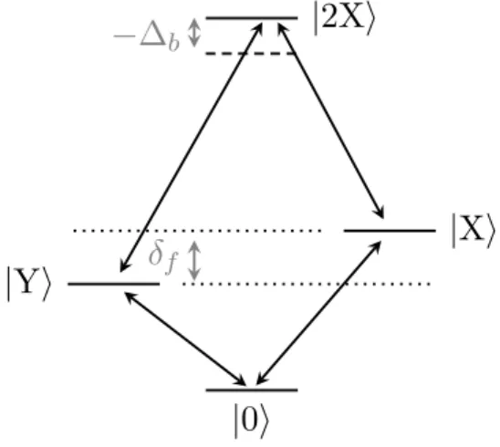
Figure 2.2: Schematic depiction of typical energy levels of an shaped single quantum dot. States|X⟩, |Y⟩
denote the energy split (by an amount δf, that is exaggerated in the figure) exciton states, whose
2 Quantum dot: Basics
confinement, the Coulombic correction to the energy for biexcitons ∆b ∼ 0 − 5 meV, is small
compared to the excitonic level splittings.
The occurrence of excitonic energy levels depend crucially on the shape and symmetry properties of the quantum dots. Under linearly polarized laser interactions, a symmetric quantum dot has exciton and bi-exciton states disposed in a four level configuration with two degenerate exciton states2. However, in an asymmetric quantum dot this degeneracy is lifted as a consequence of electron-hole exchange interactions between two otherwise degenerate exciton states (denoted by |X⟩ and |Y⟩ in Fig.[2.2]). The difference in energy of the resulting non-degenerate exciton states are referred to as fine structure splitting (δf) magnitude of which in our case∼ 0 − 500 µeV [53].
Exciton energy Hamiltonian
The resulting Hamiltonian can be represented by the four level diagonal Hamiltonian,
HQD= E0|0⟩⟨0| + EX|X⟩⟨X| + EY|Y⟩⟨Y| + E2X|2X⟩⟨2X| (2.1) where |0⟩, |X⟩, |Y⟩, |2X⟩ denotes energy states corresponding to the ground state (absence of electron-hole pair), exciton states and the biexciton state of the quantum dot respectively. Using a linearly polarized laser with polarization along one of the two crystallographic axes i.e. [110] or [1¯10] one can access either of the exciton states, which lead to a three level exciton-biexciton system representing one arm of the exciton-exciton-biexciton ladder3 (see Fig.[2.2]). The cor-responding Hamiltonian is given by:
HQD= E0|0⟩⟨0| + EX|X⟩⟨X| + E2X|2X⟩⟨2X| (2.2) which we will use in our simulations in Chapters [4,5].
2.1.2 Quantum dot-Laser Interaction
The interaction of the quantum dot with the electric field of a linearly polarized laser, which in-duces couplings between the excitonic energy levels, is described within the dipole approximation. We represent the Hamiltonian corresponding to the quantum dot-laser interaction as,
HQD−Laser=−µ0−XE(t) (
|0⟩⟨X| + |X⟩⟨0|)−µX−2XE(t) (
|X⟩⟨2X| + |2X⟩⟨X|) (2.3) where E(t) represents the electric field of the laser and µ is the dipole operator projected on the direction of laser polarization. The electric field of laser is given by,
E(t) =E(t) cos(ω0t + αt2) (2.4)
2
Though these degenerate states can be differentially accessed by employing laser with specific circular polar-ization, here we consider driving by a linearly polarized laser only
3
2.1 Introduction
which represents laser with central frequency ω0and chirp rate α evolving under the time varying profile: E(t) = Epe
−t2
τ 2p. Experimentally these pulses are obtained by passing a Fourier limited pulse of duration τ0 with a peak field strength E0 through the pulse shaping device which intro-duces a quadratic phase ϕ′′. Then the pulse duration and time varying profile of the resultant pulse are given by [54]:
τp = τ0 ( 1 +(2ϕ ′′)2 τ4 0 ) (2.5) Ep = E0 √ τ0 τp (2.6) with α = (τ42ϕ′′ 0+2ϕ′′)2
. Hence the chirped pulse is stretched and its peak field strength is reduced. We further define the pulse power:
P = ∫
dt|E(t)|2 (2.7)
which is independent of the chirp parameter and the pulse area: Θ =
∫
dt Ω(t) (2.8)
where we have defined: Ω(t) = µE(t).
2.1.3 Phonon
In periodically arranged atoms forming a lattice structure in one or more dimensions, the quan-tized normal modes of the collective motions are called phonons. These phonons offer one of the most important scattering mechanisms for electrons and holes in semiconductor heterostructures
4. Along with the omnipresent thermal vibrations, any impulsive force, for example
mechani-cal stress or electromagnetic pulses will trigger such collective motion of atoms. Decomposing the complex modes of vibrations into the normal modes offers a convenient analysis leading to the rationalization of experimental results. A simple description of their nature comes from the traditional energy vs. wavevector analysis given by dispersion relations5 Fig.[2.3]. According to their dispersion behaviour, determined by the nature of relative motions of atoms in the unit cells, these phonon modes can be classified into different subcategories [47,56]: a) Optical lon-gitudinal (LO) and transverse (TO) modes; and b) Acoutsctic lonlon-gitudinal (LA) and transverse modes (TA) . Specific roles of these individual phonon modes in the carrier scattering events can also be explained in terms of their dispersion properties. The motions within a unit cell where
4
The electron-spin interactions with the fluctuating nuclear spins bath via hyperfine effect is also a very efficient decoherence process for single electrons in quantum dots. However, due to the strong electron-hole short-range exchange interactions, which splits the optically active (bright) excitons from the non-active ones (dark excitons) by the energy of about of the order of 0.5− 1 meV in quantum dots, the exciton are protected. The hyperfine coupling terms, of the order of 50µeV for Ga, In, and As cannot therefore efficiently couple the exciton dark and bright states [55].
5
2 Quantum dot: Basics
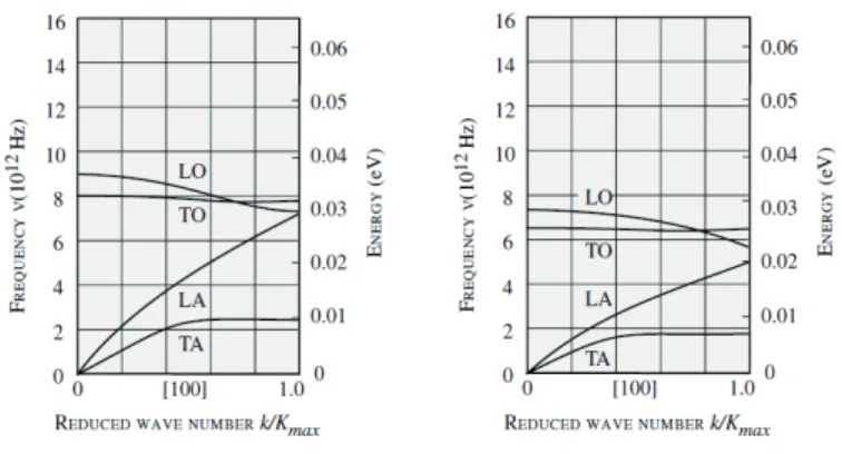
Figure 2.3: We show the typical dispersion curves from GaAs (left panel) and InAs (right panel), adapted
from Ref.[56]
neighboring atoms move in phase are referred to as coherent acoustic modes, while the relative movements of neighboring atoms out of phase are called coherent optical modes. The acous-tic modes are of lower energy compared to opacous-tical ones6 and follow a linear dispersion relation ωk,LA= cs,LA|k| (cs,LAis the speed of sound in bulk GaAs ∼ 5 × 10³m.s−1), close to the center
of the Brillouin zone. For each these modes ωk,j,{j ≡ TA1, TA2, LA, TO1, TO2, LO} there exist
one longitudinal and two transverse modes. In a series of recent experiments, these longitudinal acoustic (LA) phonon modes were identified as to be primarily responsible for exciton scattering events under strong field laser driving at low temperature ∼ 4 K [44, 45]. Henceforth we will concentrate on these particular LA phonon modes and drop the index j. Here we represent LA phonon modes surrounding the quantum dots as a collection of noninteracting harmonic oscillator modes following a Bose-Einstein distribution given by:
Nβ(ωk) =
1
eβωk− 1 (2.9)
The distribution function describes the relative abundance of LA phonon modes corresponding to energy~ωk at a temperature T = β−1/kB (where kB is the Boltzmann constant).
Phonon Hamiltonian
The Hamiltonian corresponding to the noninteracting LA phonons is then represented as, Hphonon=
∑
k
~ωkb†kbk (2.10)
6
As shown in the figure, in a typical band diagram, acoustic phonon branches occur at lower energy than the optical phonons branches. Moreover the optical branches appear flatter and the acoustic branches vanish near the center of the Brillouin zone [56]
2.1 Introduction
where b†k, bk represents the bosonic creation and annihilation operators respectively, correspond-ing to the k-th mode of energy~ωk. This independent boson model provides a sufficient
descrip-tion for our semi-empirical modeling. As mendescrip-tioned before, these LA phonon modes contribute primarily to elastic carrier scattering in quantum dot heterostructures.
2.1.4 Exciton-phonon interaction
The general nature of exciton-LA phonon interactions, in our case, involve two principle type of interactions: deformation potential coupling and piezoelectric coupling to acoustic phonon modes. InAs-GaAs dot material is weakly piezoelectric [47, 56], therefore we concentrate on the deformation potential coupling to longitudinal acoustic (LA) phonon modes only. Note that the perturbing deformation potential arises from the strain caused by motion of lattice atoms. Such interactions have been identified as the important source of phonon induced pure dephasing processes in quantum dots [45,57,58].
The general form of exciton-LA phonon coupling strength for the k-th phonon mode can be written as7 [47],
gk≡ MekF[ψe(r)]− MhkF[ψh(r)] (2.11) where,Me/hk is the matrix element corresponding to the electron-phonon/ hole-phonon interac-tion which is given as [47]:
Me/h k = |k| De/h √ 2ϱ~ωkV (2.12) where ϱ is the mass density of the host material, V is the normalization volume (which extends upto the whole sample volume) and De/his the deformation potential coupling for electron/hole taken as a constant. F[ψe/h(r)] is the form factor of the electron/hole wavefunction under the quantum dot confinement potential, taken as,
Fe/h
k [ψ
e/h(r)] =
∫
dr|ψe/h(r)|2eik·r (2.13) Assuming a spherical shape for the quantum dot and a harmonic potential confinement, the ground state wavefunction of electron/hole can be approximated as,
ψe/h(r) = e
− r2
2de/h (√πde/h)32
(2.14)
where de/h is the electron/hole ground state localization length. Since in the quantum dot samples under study, both eletrons and hole potentials have similar order of magnitude we will take: de = dh = d. Note that taking the ground state wavefunction for the electron/hole as
7In writing g
kin a factorized form, we assume that the lattice and dielectric properties of surrounding phonons
2 Quantum dot: Basics
Gaussian function is an approximation and should be exercised with caution in relation to the scattering events, especially in the low energy regime8. Also note that using a similar ground state localization length for electrons and holes is reasonable only for the strong confinement limit. Finally, the exction-LA phonon coupling strength can be written as,
gk = √ |k| 2ϱ~ωkV ( DeFk[ψe(r)]− DhFk[ψh(r)] ) = √ |k| 2ϱ~ωkV ( De ∫ dr eik.r|ψe(r)|2− Dh ∫ dr eik.r|ψh(r)|2 ) (2.15) Evaluating the integrals and squaring we get:
|gk|2=
ωk(De− Dh)2
2ϱ~c2 sV
Exp(−ω2k/ω2c) (2.16)
where we have defined, ωc = √
2cs/d as the high frequency cut-off (cs is the speed of sound in
GaAs, taken to be 5110 m.s−1 ). As it is clear from this expression, the cut-off depends on the localization length of the electron/hole which is related to the size of the quantum dot. From the estimate of the size of the InAs/GaAs quantum dots under study, we use a cut-off value: ωc= 0.72 meV.
In calculating the coupling terms we use the bulk GaAs parameters, which is a good approxi-mation in our case. We stress that these approxiapproxi-mations are valid only in the long wavelength limit of LA phonon modes (as mentioned before, all our analysis is valid for a parameter regime close to the center of Brillouin zone where linear dispersion relation for acoustic phonons hold) for which the continuum model provides a very good approximation justifying the use of bulk parameters.
Exciton-Phonon, Biexciton-Phonon interaction Hamiltonian
We introduce the exciton-phonon interaction Hamiltonian in the following form, HQD−phonon= λ { |X⟩⟨X|∑ k ( gkb†k+ g∗kbk)+ 2|2X⟩⟨2X|∑ k ( gkb†k+ g∗kbk)} (2.17)
The interaction Hamiltonian is taken in a bilinear form: HQD−phonon = λ (S ⊗ B), where S and B corresponds to excitonic system and bath coupling operator respectively,
S = |X⟩⟨X| + 2 |2X⟩⟨2X| (2.18)
B = ∑
k
(
gkb†k+ g∗kbk) (2.19)
and λ is a scaling parameter whose magnitude determines the strength of coupling9. For the biLA phonon interaction, we use a coupling constant two times that of the
exciton-8
For a recent article discussing this approximation, see [59]. 9
2.2 Notion of Open quantum system
phonon, and keep the diagonal form for the excitonic part of the interaction operator10. The coupling strengths to k-th phonon mode is denoted by gk and given by Eq.[2.15].
2.2 Notion of Open quantum system
Traditionally, the system of investigation which exchange particles and energy with other systems during the course observation are classified as open quantum systems. The motivation can be ascribed to practical situations, where we are almost always interested in some specific variables (or degrees of freedom) in a system as observables which are invariably interacting with the remaining variables during a physical process. Therefore, while exploring the dynamics of such systems one is encountered with the conceptual need to establish a formal partitioning between the variables of interest and variables of secondary interest in order to analyze them with dis-criminating rigor and accuracy. Subsystem specifies a part of the whole physical system which contains the relevant while Bath or reservoir indicates to those irrelevant dynamical variables whose dynamics are not of primary interest. This partitioning is almost always physically mo-tivated and depends on the specific system and properties one is interested in. The microscopic description of dynamics thereafter involves identifying the nature interaction between the system and the bath and describing the time evolution of the system. We are specifically interested in the observables related to quantum dot excitonic dynamics which interacts with surrounding phonon degrees of freedom while the laser driving is on. Therefore, we formalize the context in which the methods of open quantum systems will be applied in our problem. We classify the quantum dots interacting with the laser as system which interacts with the LA phonon modes classified as bath through the interactions mediated by system-bath coupling terms. This motivates us to define the total microscopic Hamiltonian corresponding to the system under study in the next section.
2.3 The microscopic Hamiltonian
The full Hamiltonian consists of terms corresponding to the quantum dot system, the LA phonon bath, and the exciton-LA phonon interaction taking the form,
HT = HQD+HQD−laser+Hphonon+HQD−phonon = H0+Hint+Hb+Hsb
= Hs+Hb+Hsb (2.20)
where we have identified: H0 ≡ HQD;Hb ≡ Hphonon;Hsb ≡ HQD−phonon;Hint ≡ HQD−laser. Furthermore we take: Hs=H0+Hint including the laser driving into the system Hamiltonian.
This is suitable for describing dissipation in a dressed state picture.
10In the case of strongly confined quantum dots, for small number of carriers, the electron/hole envelope functions do not depend strongly on the number of carriers within the quantum dots.
2 Quantum dot: Basics
Exciton-Biexciton Hamiltonian
The full microscopic Hamiltonian of the biexciton-laser-phonon system can be represented in a concise form as,
HT = Hs+Hb+Hsb = E0|0⟩⟨0| + EX|X⟩⟨X| + E2X|2X⟩⟨2X| − µ0−XE(t) { |0⟩⟨X| + |X⟩⟨0| } − µX−2XE(t) { |X⟩⟨2X| + |2X⟩⟨X| } + ∑ k ~ωkb†kbk+ λ { |X⟩⟨X|∑ k ( gkb†k+ gk∗bk)+ 2|2X⟩⟨2X|∑ k ( gkb†k+ g∗kbk)}(2.21)
where the symbols have their usual meanings defined before.
Exciton Hamiltonian
Furthermore, if one restricts the laser bandwidth so as to evade the biexciton transition and chooses a suitable laser polarization, it is possible to access the exciton transition only. The system can then be modeled as a two level system and the corresponding Hamiltonian can be represented as, HT = Hs+Hb+Hsb = E0|0⟩⟨0| + EX|X⟩⟨X| − µ0−XE(t) { |0⟩⟨X| + |X⟩⟨0| } + ∑ k ~ωkb†kbk+ λ|X⟩⟨X| ∑ k ( gkb†k+ gk∗bk) (2.22)
Thus we have defined all the effective, working Hamiltonians that describe the relevant processes of interest. In several of the previous analysis published [45,60] similar Hamiltonians were used to analyze the exciton dynamics in relations to quantum dot laser interactions.
3 Non-Markovian dynamics in quantum dots :
Formalisms
3.1 Introduction
Here we develop the necessary formalisms for non Markovian master equation that will describe the excitonic dynamics corresponding to the Hamiltonians presented in the previous chapter. We will take up the projection operator formalism developed in [61,62] which has been successfully employed in the past to obtain generalized master equations for the reduced density matrix. In particular, we will develop a master equation using the auxiliary density matrix method based on a special parametrization of bath spectral density introduced in [63]. The resulting time local coupled set of equations are amenable to straightforward numerical solutions.
3.2 Generalized master equation
3.2.1 Projector operator formalism
The time dependence of the full density operator, is governed by the Liouville-von Neumann equation of the full system-bath density matrix: ρT(t),
∂tρT(t) =−i[HT(t),ρT(t)]≡ LT(t)ρT(t) (3.1) where the second equivalence is due to the introduction of the Liouville superoperator notation: LT=Ls+Lb+Lsb. Our motivation is to introduce a formal partitioning of the density operator
in order to be able to analyze the dynamics of the relevant variables in terms of reduced density matrix. Hence, we introduce the projection superoperator: P and the complementary: Q=1 − P. Using these projection superoperators, the total density operator can be partitioned in the following mutually exclusive summands: density operator containing ’relevant’ variables and ’non-relevant’ variables.
ρT(t) =PρT(t) +QρT(t) (3.2)
Hereafter, we want a dynamical equation for the relevant part of the density operator only. While, the dynamical effects of the non-relevant part will be included by one of the several available
3 Non-Markovian dynamics in quantum dots : Formalisms
schemes. Inserting Eq.[3.2] back into the von Neumann equation, we obtain a coupled set of differential equations,
∂tPρT(t) = PLPρT(t) +PLQρT(t)
∂tQρT(t) = QLPρT(t) +QLQρT(t) (3.3) which formally express the dynamical evolution for the relevant part (PρT) and non-relevant part (QρT) of the density operator, respectively. Note that they affect each other dynamically and by working with on any one of them would lead to non locality as we are working in a reduced space of variables. Solving these coupled equations formally lead to:
∂tPρT(t) =PLPρT(t) +PLT e ∫t t0dt′QLQρ T(t0) + ∫ t t0 dt′PLT e∫t′tdt′′QLQLPρ T(t′) (3.4) where we have used time ordering operator: T necessary to allow an explicit time dependent Liouvillian. The equation above is a formal and exact expression of the time evolution of the relevant part of the density operator. However, to proceed further, the projector needs to be defined, depending to the specific problem at hand.
3.2.2 Context of the problem
We introduce the particular form of the Nakajima-Zwanzig projection superoperator:
P(·) = Br⊗ Trb(·) (3.5)
where (·) denotes the operand the projector acts upon. As can be seen, the projector, acting on the full density operator, separates it into direct product subspaces containing subsystem density operator (or reduced density operator) and a reference bath density operator. The reference state of bath, given by: Br is taken to be in the thermal equilibrium1 i.e. Br≈ B0 ≡ ρeqb where,
ρeqb = 1 Zb
e−βHb with Tr
b(ρeqb ) = 1 (3.6)
Introducing the projector, in Eq.[3.4], we get, B0Trb{∂tρT(t)} = B0Trb{LPρ(t)} + B0Trb{LT e ∫t t0dt′QLQρT(t0) + ∫ t t0 dt′B0Trb{LT e ∫t t′dt′′QLQρT(t′)} ∂tρ(t) = Trb{LPρT(t)} + Trb{LT e ∫t t0dt′QLQρ T(t0) + ∫ t t0 dt′Trb{LT e ∫t t′dt′′QLQρT(t′)} (3.7) This equation presents the time evolution of subsystem density operator. Here, the first term de-scribes the dynamics under an effective Liouvillian as: LeffρT(t) = Trb{LPρ(t)} using: Trb{ρT(t)} =
1
This is an approximation which is valid in our case. However caution should be taken in extrapolating such assumption to other situations where an initially correlated bath cannot be replaced by an equilibrium one as highlighted in [63,64].
3.2 Generalized master equation
ρ(t). The second term represents the influence from the subsystem-bath correlation at initial time referred to as initial correlation: I(t) = Trb{LT e
∫t
t0dt′QLQρ
T(t0). Here we assume that prior to the laser interaction at t0, we have ρT(t0) = ρeqb |0⟩⟨0|, which leads to I = 0. Further, in the Appendix [3.3.1], it is shown that in our case, we haveLeff =Ls. The third term accounts for the
influence of subsystem-bath dynamical correlation and is called memory kernel: K(t − t′)ρ(t′). The simplification of this term is more involved, and requires further developments which will be detailed in the next section.
3.2.3 Evaluation of Memory Kernel
We start with the definition:
K(t − t′)ρ(t′) = Tr b{LT e
∫t
t′dt′′QLQLB0ρ(t′)} (3.8) which following the simplification in Appendix[3.3.2], takes the form,
K(t − t′)ρ(t′) = −λ2[S, T e∫t′tdt′′LsSρ(t′)Trb{ei(t−t′)HbBe−i(t−t′)HbBB0}
− T e∫t′tdt′′Lsρ(t′)S Trb{ei(t−t′)HbBe−i(t−t′)HbBB0}] (3.9) Introducing the bath correlation function: C(α) = Trb{eαHbBe−αHbBB0} where α = i(t − t′) the memory term can be re-written in a simplified form as:
K(t − t′)ρ(t′) = iλ2[S, iC(t − t′)T e∫t′tdt′′LsSρ(t′) | {z } I −iC∗(t− t′)T e∫t t′dt′′Lsρ(t′)S | {z } II ] (3.10) The effect of bath therefore enters the subsystem dynamics through the bath correlation function. Note that the term [II] is the hermitian conjugate of term [I], which will be utilized later for the development of an efficient numerical procedure for solving the non-Markovian master equation.
3.2.4 Bath correlation function
The general bath correlation function appearing in the memory kernel of the master equation has the following form:
C(α) = Trb{eαHbBe−αHbBB0} (3.11)
However this is a formal equation and needs to be evaluated further by defining the bath Hamil-tonian: Hb and the bath operator: B in the context of the problem at hand. Therefore, we will
evaluate the bath correlation function by insertingHb and B defined in Eq.[2.10,2.19], Hb = ∑ k ωkb†kbk B = ∑ k (gkb†k+ g∗kbk)
3 Non-Markovian dynamics in quantum dots : Formalisms
Following a simplification (see Appendix[3.3.3]) it takes the form, C(α) =∑ k ( eαωkN β(ωk)|gk|2+ e−αωk(Nβ(ωk) + 1)|gk|2 ) (3.12)
Further, in the limit of infinitely many oscillators, assuming a continuous variation of spectral distribution function over frequencies, we write,
C(α) = ∫ ∞ 0 dω ( J (ω) eβω− 1− J (−ω)e−αω 1− eβω ) = ∫ ∞ −∞dωJ (ω) ( eαω eβω− 1 ) (3.13) where we have introduced, J (ω) = ∑k|gk|2δ(ω − ωk). In finding the form of J (ω) we use the
following replacement (which amounts to transferring the integral from k-space to energy space), ∑ k → V (2π)3 ∫ d3k (3.14)
Also using the relation from Eq.[2.16] i.e. |gk|2 = ωk|De−Dh|
2 2πϱcs2V Exp(−ω 2 k/ωc2), we find: J (ω) = ∑ k |gk| 2 δ(ω− ωk) = |De− Dh| 2 4π2ϱc5 s ∫ ∞ 0 dωkωk3Exp(−ω2k/ωc2) δ(ω− ωk) = A ω3e− ( ω ωc )2 (3.15) Thus we have the spectral distribution function of the form:
J (ω) = A ω3e− ( ω ωc )2 (3.16) with the parameter A that depends on the parameters from the microscopic model and the physical properties of the substrate,
A = |De− Dh| 2
4π2ϱc5 s
(3.17) The value of A used in the simulation is given in Appendix [3.3.5]. Note that the spectral distribution function is super-ohmic in nature where the low frequency behavior is governed by a power law and the high frequency tail is truncated by the cut-off ωc. This is commensurate
with the physical behavior of LA phonons in the relevant parameter regime.
We again stress, that in the calculation of the the coupling parameter it is found that the bulk GaAs parameters provide a good estimate for the surrounding material of the embedded quantum dot.
3.2 Generalized master equation
3.2.5 Parametrization of bath spectral density
One of the key ingredient of the non-Markovian master equation that we are developing is the parametrization of the bath spectral distribution function [63, 65, 66] given by Eq.[3.16]. We represent the bath spectral density as:
J (ω) = A ω3e− ( ω ωc )2 ≡ n ∑ l=1 p(l)j(l)(ω) (3.18) where, j(l)(ω) = ω 3 [(ω + Ω(l)1 )2+ Γ(l) 1 2 ][(ω− Ω(l)1 )2+ Γ(l) 1 2 ][(ω + Ω(l)2 )2+ Γ(l) 2 2 ][(ω− Ω(l)2 )2+ Γ(l) 2 2 ] (3.19)
The parametrization is generally introduced via numerical fitting procedures which determines the number of terms to be included in the sum. In our treatment, we use 4 terms in the summand for a sufficiently accurate fitting. Taking sum of products of Lorentzians allows one to perform the integration over J (ω) in Eq.[3.13] analytically by contour integration. Each term under the summation in Eq.[3.19] has 4 poles in the upper complex plane corresponding to Im[α] > 0, and an infinite number of poles at the Matsubara frequencies: νm = 2π mβ stemming from Nβ. Then
the correlation function can be expressed as a sum of exponentials:
C(t − t′) = 2πi n ∑ l=1 p(l) 4 ∑ κ=1 Nβ ( G(l)κ ) Res G(l)κ [ j(l)(ω) ] eiG(l)κ (t−t′) + 2πi β ∞ ∑ m=1 J (iνm)e−νk(t−t ′) (3.20) with G(l)1 = Ω(l)1 + iΓ(l)1 G(l)2 = −Ω(l)1 + iΓ(l)1 G(l)3 = Ω(l)2 + iΓ(l)2 G(l)4 = −Ω(l)2 + iΓ(l)2 (3.21)
3 Non-Markovian dynamics in quantum dots : Formalisms and ResG(l) 1 [ j(l)(ω) ] = −iG (l) 1 2 8Ω(l)1 Γ(l)1 {( G(l)1 )4 + 2 ( G(l)1 )2[( Γ(l)2 )2 −(Ω(l)2 )2] + [( Γ(l)2 )2 + ( Ω(l)2 )2]2 }−1 ResG(l) 2 [ j(l)(ω) ] = iG (l) 2 2 8Ω(l)1 Γ(l)1 {( G(l)2 )4 + 2 ( G(l)2 )2[( Γ(l)2 )2 −(Ω(l)2 )2] + [( Γ(l)2 )2 + ( Ω(l)2 )2]2}−1 ResG(l) 3 [ j(l)(ω) ] = −iG (l) 3 2 8Ω(l)2 Γ(l)2 {( G(l)3 )4 + 2 ( G(l)3 )2[( Γ(l)1 )1 −(Ω(l)1 )2] + [( Γ(l)1 )2 + ( Ω(l)1 )2]2}−1 ResG(l) 4 [ j(l)(ω) ] = iG (l) 4 2 8Ω(l)2 Γ(l)2 {( G(l)4 )4 + 2 ( G(l)4 )2[( Γ(l)1 )2 −(Ω(l)1 )2] + [( Γ(l)1 )2 + ( Ω(l)1 )2]2}−1 (3.22) We re-write the correlation function, in a concise form:
C(t − t′) = ∑∞ k=1
Λkeiγk(t−t
′)
(3.23)
where Λk and γk are given by direct comparison with Eq.[3.20]. This property will be used to
deconvolute the memory kernel, in order to obtain a coupled set equations in terms of effective density matrices. This approach, termed Auxiliary density matrix method [40, 63,65–67], is detailed in the next section.
3.2.6 Auxiliary density matrix method
To begin with, we re-write the time evolution of reduced density matrix,
˙ ρ(t) = Lsρ(t) + ∫ t t0 dt′K(t − t′)ρ(t′) = Lsρ(t) + iλ2 ∫ t t0 dt′[S, iC(t − t′)T e ∫t t′dt′′LsSρ(t′)− iC∗(t− t′)T e− ∫t t′dt′′Lsρ(t′)S] (3.24) We define auxiliary density matrices by:
ρk(t) = iΛk
∫ t t0
dt′eγk(t−t′)T e∫t′tdt′′LsSρ(t′) (3.25)
which allows us to write:
˙ ρ(t) = Lsρ(t) + iλ2 ∞ ∑ k=1 [ S, ρk(t) + ρ†k(t) ] (3.26)
3.3 Appendix
where we have used the fact that term II in Eq.[3.9] is the hermitian conjugate of Eq.[3.25]. The auxiliary density matrices themselves can be calculated alongside with ρ on the fly. Indeed, from Eq.[3.25,3.26], one finds that ρ and the ρk obey a system of coupled differential equations:
˙ ρ(t) = Lsρ(t) + iλ2 ∞ ∑ k=1 [ S, ρk(t) + ρ†k(t) ] ˙ ρk(t) = { Ls+ γk } ρk(t) +Sρ(t) k = 1,∞ (3.27)
This set of coupled Liouville equations takes memory effects fully into account, since it is equiv-alent to Eq.[3.7]. In practice, a finite number of auxiliary density matrices are used and the coupled set of equations is solved using a standard Runge-Kutta integrator. Thus in deriving these working equations, we have avoided the time non-locality in the non Markovian master equation Eq.[3.24] by expanding the space of parameters, by introducing a set of auxiliary den-sity matrices.
3.3 Appendix
3.3.1 Simplification of effective Liouvilian term
Here we simplify the effective Liouvillian term. LeffρT(t) = Trb{LB0ρT(t)}
= Trb{(Ls+Lb+ λLsb)B0ρT(t)}
= Trb{LsB0ρT(t)} + Trb{LbB0ρT(t)} + Trb{λLsbB0ρT(t)}
= Lsρ(t) (3.28)
where we have used the fact that the coupling Hamiltonian is bilinear.
3.3.2 Simplification of memory kernel term
Here we proceed to simplify the term corresponding to the memory kernelK(t − t′) Eq.[3.8]. In doing so we will employ perturbation expansion in system-bath coupling strength to the second order. To simplify the notation, we define: L0=Ls+Lb
K(t − t′)ρ(t′) = Tr b{LT e ∫t t′dt′′QLQLPρ(t′)} = Trb{(L0+ λLsb)T e ∫t t′dt′′Q(L0+λLsb)Q(L 0+ λLsb)Pρ(t′)} = λTrb{LsbT e ∫t t′dt′′Q(L0+λLsb)(QL 0P + λQLsbP)ρ(t′)} = λ2Trb{LsbT e ∫t t′dt′′QL0QLsbPρ(t′)} = λ2Trb { LsbT e ∫t t′dt′′QL0(LsbP − PLsbPρ(t′))} (3.29)
3 Non-Markovian dynamics in quantum dots : Formalisms
Further simplifying the term,T e∫t′tdt′′QL0LsbPρ(t′) as,
T e∫t′tdt′′QL0LsbPρ(t′) = T e∫t′tdt′′(1−P)L0LsbPρ(t′) = { 1 + ∫ t t′ dt′′(L0− PL0) +1 2 ∫ t t′ dt′′ ∫ t′′ t′′′ dt′′′(L0− PL0)(L0− PL0) + . . . } LsbPρ(t′) = { 1 + ∫ t t′ dt′(L0− L0P) +1 2 ∫ t t′ dt′′ ∫ t′′ t′′′ dt′′′(L0− L0P)(L0− L0P) + . . . } LsbPρ(t′) = { LsbP + ∫ t t′ dt′ ( L0LsbP − L0PL| {z }sbP =0 ) +1 2 ∫ t t′ dt′′ ∫ t′′ t′′′ dt′′′(L0− L0P) ( L0LsbP − L0PL| {z }sbP =0 ) + . . . } ρ(t′) = { LsbP + ∫ t t′ dt′L0LsbP + 1 2 ∫ t t′ dt′′ ∫ t′′ t′′′ dt′′′(L0− L0P)L0LsbP + . . . } ρ(t′) = { LsbP + ∫ t t′ dt′L0LsbP + 1 2 ∫ t t′ dt′′ ∫ t′′ t′′′ dt′′′ ( L0L0LsbP − L0PL| {z }0LsbP =0 ) + . . . } ρ(t′) = { 1 + ∫ t t′ dt′L0+ 1 2 ∫ t t′ dt′′ ∫ t′′ t′′′ dt′′′L0L0+ . . . } LsbPρ(t′) = T e∫t′tdt′′L0LsbPρ(t′) (3.30)
Inserting back in Eq.[3.29], we get, K(t − t′)ρ(t′) = λ2Trb{LsbT e ∫t t′dt′′L0LsbPρ(t′)} = −iλ2Trb{LsbT e ∫t t′dt′′L0(t−t′)[Hsb,Pρ(t′)]} = −iλ2Trb{LsbT e ∫t t′dt′′LseLb(t−t′)[SB,B0ρ(t′)]} = −iλ2Trb { Lsb ( T e∫t′tdt′′LsSρ(t′)eLb(t−t′)BB0− eLb(t−t′)B0BT e ∫t t′dt′′Lsρ(t′)S )} = −iλ2Trb { [ Hsb, ( T e∫t′tdt′′LsSρ(t′)eLb(t−t′)BB 0− eLb(t−t ′) B0BT e ∫t t′dt′′Lsρ(t′)S )] } = −λ2Trb { [ S,(T e∫t′tdt′′LsSρ(t′)B eLb(t−t′)BB 0− BeLb(t−t ′) B0B T e ∫t t′dt′′Lsρ(t′)S )] } = −λ2 [ S,T e∫t′tdt′′LsSρ(t′)Trb{BeLb(t−t′)BB 0 } − Trb { BeLb(t−t′)B 0B } T e∫t′tdt′′Lsρ(t′)S ] (3.31) This form corresponds to Eq.[3.9].
3.3 Appendix
3.3.3 Bath correlation function
Here, we detail the simplification of the time correlation function, in the context of our problem by bringing in the bath Hamiltonian and system-coupling operator.
C(α) = Trb { eα∑kωkb † kbkBe−α ∑ kωkb † kbkBB0 } = Trb { eα∑kωkb†kbk∑ k (gkb†k+ g∗kbk)e−α ∑ ωkb†kbk∑ k (gkb†k+ gk∗bk)B0 } = Trb { ∑ k ∑ k′ ( eα∑kωkb†kbkg kb†ke−α ∑ k′ωk′b†k′bk′g k′b†k′+ e−α ∑ k′ωkb†kbkg kb†ke−α ∑ k′ωk′b†k′bk′g∗ k′bk′ + eα∑kωkb†kbkg∗ kbke−α ∑ k′ωk′b†k′bk′g k′b†k′+ eα ∑ kωkb†kbkg∗ kbke−α ∑ k′ωk′b†k′bk′g∗ k′bk′ ) B0 } = Trb { ∑ k δkk′ ( eα∑kωkb†kbkg kb†ke−α ∑ k′ωk′b†k′bk′g k′b†k′+ e−α ∑ k′ωkb†kbkg kb†ke−α ∑ k′ωk′b†k′bk′g∗ k′bk′ + eα∑kωkb†kbkg∗ kbke−α ∑ k′ωk′b†k′bk′g k′b†k′+ e α∑kωkb†kbkg∗ kbke−α ∑ k′ωk′b†k′bk′g∗ k′bk′ ) B0 } =∑ k |gk|2 { e−αωk⟨b† kb†k⟩β+ eαωk⟨bkb†k⟩β+ e−αωk⟨b†kbk⟩β+ eαωk⟨bkbk⟩β } (3.32)
In determining the above expression we have used following identities [68]: e−λb†bb† = e−λb†e−λb†b
e−λb†bb = eλbe−λb†b (3.33)
and the following relations [68],
δkk′⟨b†kb†k′⟩β = 0
δkk′⟨bkbk′⟩β = 0 (3.34)
Moreover using the following replacement rules which follows from Bose-Einstein statistics [68], ⟨b†kbk⟩β ≡ Nβ(ωk) = 1 eβωk− 1 ⟨bkb†k⟩β ≡ Nβ(ωk) + 1 = eβωk eβωk− 1 (3.35) we can obtain, C(α) =∑ k ( eαωkN β(ωk)|gk|2+ e−αωk(Nβ(ωk) + 1)|gk|2 ) (3.36)
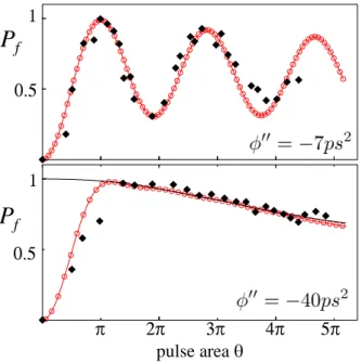
![Figure 4.3: Numerical simulation of the exciton population, (Eq.[ 4.5 ]) compared to the analytical ex- ex-pression (Eq.[ 4.34 ]), full black line) for different temperatures, as indicated](https://thumb-eu.123doks.com/thumbv2/123doknet/2228819.15846/47.892.252.599.141.480/numerical-simulation-population-analytical-pression-different-temperatures-indicated.webp)