Improvement of cross section model in COCAGNE code of the calculation chain of EDF

(1)

HAL Id: tel-01630268

https://tel.archives-ouvertes.fr/tel-01630268

Submitted on 7 Nov 2017

HAL is a multi-disciplinary open access

archive for the deposit and dissemination of sci-entific research documents, whether they are pub-lished or not. The documents may come from teaching and research institutions in France or abroad, or from public or private research centers.

L’archive ouverte pluridisciplinaire HAL, est destinée au dépôt et à la diffusion de documents scientifiques de niveau recherche, publiés ou non, émanant des établissements d’enseignement et de recherche français ou étrangers, des laboratoires publics ou privés.

of the calculation chain of EDF

Thi Hieu Luu

To cite this version:

Thi Hieu Luu. Improvement of cross section model in COCAGNE code of the calculation chain of EDF. Mathematical Physics [math-ph]. Université Pierre et Marie Curie - Paris VI, 2017. English. �NNT : 2017PA066120�. �tel-01630268�

(2)

Thèse de doctorat de

l’Université Pierre et Marie Curie

Spécialité

Mathématiques Appliquées

présentée par

Thi Hieu LUU

pour obtenir le grade de

DOCTEUR de l’UNIVERSITÉ PIERRE ET MARIE CURIE

Amélioration du modèle de sections efficaces dans le code

de cœur COCAGNE de la chaîne de calculs d’EDF

Soutenue le 17/02/2017

Directeur de thèse : _{M. Yvon MADAY} Professeur, Université Pierre et Marie Curie Encadrants de thèse : _{M. Matthieu GUILLO} Ingénieur - Chercheur, EDF - R&D

M. Pierre GUÉRIN Ingénieur - Chercheur, EDF - R&D Rapporteurs : _{M. Anthony NOUY} Professeur, École Centrale de Nantes

M. Lars GRASEDYCK Professeur, RWTH Aachen University Examinateurs : _{M. Albert COHEN} Professeur, Université Pierre et Marie Curie

M. Daniele TOMATIS Chercheur, CEA M. Andrea ZOIA Chercheur, CEA

(3)

(4)

Thèse effectuée aux :

Laboratoire Jacques-Louis Lions, UMR 7598 Adresse géographique :

Laboratoire Jacques Louis Lions 3ème étage, tour 15-16, 15-25, 16-26 4 place Jussieu

75005 Paris, France

+33 (0)1 44 27 42 98 (Tél.) Adresse postale :

Laboratoire Jacques-Louis Lions Université Pierre et Marie Curie Boîte courrier 187

75252 Paris Cedex 05 France

Département SINETICS, EDF - R&D Adresse :

Département SINETICS EDF Lab Paris - Saclay 7, Boulevard Gaspard Monge 92120 Palaiseau, France

(5)

(6)

Résumé

Afin d’exploiter au mieux son parc nucléaire, la R&D d’EDF est en train de développer une nouvelle chaîne de calcul pour simuler le cœur des réacteurs nucléaires avec des outils à l’état de l’art. Ces calculs nécessitent une grande quantité de données physiques, en particulier les sections efficaces.

Dans la simulation d’un cœur complet, le nombre de valeurs des sections efficaces est de l’ordre de plusieurs milliards. Ces sections efficaces peuvent être représentées comme des fonctions multivariées dépendant de plusieurs paramètres physiques. La détermination des sections efficaces étant un calcul complexe et long, nous pouvons donc les précalculer en certaines valeurs des paramètres (caluls hors ligne) puis les évaluer en tous points par une interpolation (calculs en ligne). Ce processus demande un modèle de reconstruction des sections efficaces entre les deux étapes.

Pour réaliser une simulation plus fidèle du cœur dans la nouvelle chaîne d’EDF, les sections efficaces nécessitent d’être mieux représentées en prenant en compte de nouveaux paramètres. Par ailleurs, la nouvelle chaîne se doit d’être en mesure de calculer le réacteur dans des situations plus larges qu’actuellement. Le modèle d’interpolation multilinéaire pour reconstruire les sections efficaces est celui actuellement utilisé pour répondre à ces objectifs. Néanmoins, avec ce modèle, le nombre de points de discrétisation augmente exponentiellement en fonction du nombre de paramètres ou de manière considérable quand on ajoute des points sur un des axes. Par conséquence, le nombre et le temps des calculs hors ligne ainsi que la taille du stockage des données deviennent problématique. L’objectif de cette thèse est donc de trouver un nouveau modèle pour répondre aux demandes suivantes : (i)-(hors ligne) réduire le nombre de précalculs, (ii)-(hors ligne) réduire le stockage de données pour la reconstruction et (iii)-(en ligne) tout en conservant (ou améliorant) la précision obtenue par l’interpolation multilinéaire.

D’un point de vue mathématique, ce problème consiste à approcher des fonctions multivariées à partir de leurs valeurs précalculées. Nous nous sommes basés sur le format de Tucker - une approx-imation de tenseurs de faible rang afin de proposer un nouveau modèle appelé la décomposition de Tucker. Avec ce modèle, une fonction multivariée est approchée par une combinaison linéaire de pro-duits tensoriels de fonctions d’une variable. Ces fonctions d’une variable sont construites grâce à une technique dite de décomposition en valeurs singulières d’ordre supérieur (une “matricization” com-binée à une extension de la décomposition de Karhunen-Loève). L’algorithme dit glouton est utilisé pour constituer les points liés à la résolution des coefficients dans la combinaison de la décomposition de Tucker.

Les résultats obtenus montrent que notre modèle satisfait les critères exigés sur la réduction de données ainsi que sur la précision. Avec ce modèle, nous pouvons aussi éliminer a posteriori et a priori les coefficients dans la décomposition de Tucker. Cela nous permet de réduire encore le stockage de données dans les étapes hors ligne sans réduire significativement la précision.

Mots-clés : sections efficaces, décomposition de Tucker, approximation de tenseurs de faible rang, décomposition en valeurs singulières d’ordre supérieur, algorithme glouton, neutronique, ré-duction de modèle, sparse grids

(7)

(8)

Abstract

In order to optimize the operation of its nuclear power plants, the EDF’s R&D department is currently developing a new calculation chain to simulate the nuclear reactors core with state of the art tools. These calculations require a large amount of physical data, especially the cross-sections.

In the full core simulation, the number of cross-section values is of the order of several billions. These cross-sections can be represented as multivariate functions depending on several physical parameters. The determination of cross-sections is a long and complex calculation, we can therefore pre-compute them in some values of parameters (offline calculations), then evaluate them at all desired points by an interpolation (online calculations). This process requires a model of cross-section reconstruction between the two steps.

In order to perform a more faithful core simulation in the new EDF’s chain, the cross-sections need to be better represented by taking into account new parameters. Moreover, the new chain must be able to calculate the reactor in more extensive situations than the current one. The multilinear interpolation is currently used to reconstruct cross-sections and to meet these goals. However, with this model, the number of points in its discretization increases exponentially as a function of the number of parameters, or significantly when adding points to one of the axes. Consequently, the number and time of offline calculations as well as the storage size for this data become problematic. The goal of this thesis is therefore to find a new model in order to respond to the following requirements: (i)-(offline) reduce the number of pre-calculations, (ii)-(offline) reduce stored data size for the reconstruction and (iii)-(online) maintain (or improve) the accuracy obtained by multilinear interpolation.

From a mathematical point of view, this problem involves approaching multivariate functions from their pre-calculated values. We based our research on the Tucker format - a low-rank tensor approximation in order to propose a new model called the Tucker decomposition. With this model, a multivariate function is approximated by a linear combination of tensor products of one-variate functions. These one-variate functions are constructed by a technique called higher-order singular values decomposition (a “matricization” combined with an extension of the Karhunen-Loeve decom-position). The so-called greedy algorithm is used to constitute the points related to the resolution of the coefficients in the combination of the Tucker decomposition.

The results obtained show that our model satisfies the criteria required for the reduction of the data as well as the accuracy. With this model, we can eliminate a posteriori and a priori the coefficients in the Tucker decomposition in order to further reduce the data storage in offline steps but without reducing significantly the accuracy.

Keywords: cross-sections, Tucker decomposition, low-rank tensor approximation , higher-order singular value decomposition, greedy algorithm, neutronics, reduced model, sparse grids

(9)

(10)

Acknowledgements

Time always goes by so fast and the moment has come after three years for this thesis to end. I am writing these lines to express my acknowledgment to the people who helped me and accompanied me throughout of this memorable period. Without their support, my work could not have been accomplished.

First, let me express my deepest gratitude to my supervisor, Professor Yvon MADAY, at the Laboratoire Jacques Louis Lions (LJLL). Yvon, you are the person who led me to this thesis (by chance) and you are also the person who guided me through the important progress in my work. Without your patience, your enthusiasm and above all, your extensive scientific knowledge, I would not have got the results I have today. Although very busy, Yvon still reserved his precious time to follow my work and to help me when I needed it. Thank you so much for what you did for me.

The most sincerest and deepest thanks I also give to my two industrial supervisors: Matthieu GUILLO and Pierre GUÉRIN, at EDF - R&D. I was very lucky to have two very competent in-dustrial supervisors in two complementary domains: Matthieu for neutronic physics and Pierre for mathematics. Thank you both for trusting me in this work despite all my defects that you knew. Matthieu and Pierre, you have both always been my references for any technical and administrative problem. Your guidance and your advice have helped me enormously in the organization of my work and in the progress of this thesis. Your availability, your patience and your time reserved for my work, all are immeasurable.

I would like to thank all the members of the jury: Professor Anthony NOUY and Professor Lars GRASEDYCK for having accepted to be the reviewers of this thesis, for having conscientiously read my work and having spent your time to write the constructive reports. My sincere thanks also goes to Professor Albert COHEN, researcher Daniele TOMATIS and researcher Andrea ZOIA for your examination as well as your interest in my work.

This research was done in EDF’s SINETICS department and the LJLL laboratory of Université Pierre et Marie Curie. I would like to thank these two establishments for hosting me during the entire research period. In particular, I would like to express my gratitude to the group leader of I27 at EDF: Philippe MAGAT, and the head of the SIMUCOEUR2 project, Coline BROSSELARD.

(11)

A very big thanks is expressed to Nadine SCHWARTZ who has helped me a lot with the instal-lation and the utilization of GAB. It would have been hard to accomplish this work without your guidance. Nadine also provided me with many documents on her research and methods related to the problem in my thesis, which gave me a better overview of my work.

I would also like to thank Serge MARGUET for your enthusiasm and patience in enlightening me with knowledge about neutron equations. Also, many thanks to Angelique PONCOT for your documents on Areva’s model.

Special thanks to Ansar CALLOO for your discussions as well as your advice about writing the first journal paper in a PhD thesis. Thanks to Nathalie GULER for the times you picked me up to go to work. Thanks to Hélène MONDAIN for your interest in Vietnam, for your kindness. Thanks to Florian HAURAIS for sharing with me our office.

And sincere thanks to the two groups I27, I28, who always created a friendly environment full of humor with many delicious homemade cakes and picnic meetings.

I now think about my husband, Thanh-Hà and my two sons Hugo and Louis. A lot of emotion when I write about my small family. A person once asked me how I can do this thesis with my two little sons beside me? It would not be true if I said that there was no difficulty. But above all, my husband and my two sons are the ones who are always beside me, encourage me, balance my emotions. My husband is not only the one who shares with me all the troubles in my life but also the one who guides me with patience on scientific research. There is no word to express the importance of my family in my heart.

Finally, a huge thanks and deep gratitude to all members of my family in Vietnam. Thanks to my parents who always supported me before, during and even after this thesis. The presence of my parents-in-law, me. Thanh and b´ô Dân, at this moment with their help in my daily work is unmeasurable for this final stage. The support of “em Lân” is also very important so the word “thank you” is never enough. For my sisters: H`ăng, Nga, Tha’o, this PhD thesis is a gift I dedicate to you.

(12)

Introduction (Version française)

Motivation

EDF est le premier électricien du monde, grâce notamment à son parc français composé de 58 réacteurs nucléaires à eau pressurisée (REP). Afin de piloter et contrôler le fonctionnement de ces réacteurs, EDF a développé des chaînes de calcul qui simulent le comportement du cœur d’un réacteur. Face aux demandes de plus en plus exigeantes de l’ingénierie en termes de temps de calcul et de précision, une nouvelle chaîne de calcul de cœur, appelée ANDROMEDE, est en cours de développement à EDF-R&D.

L’un des éléments de la chain est le code neutronique, appelé COCAGNE, dont l’un des objectifs est de résoudre numériquement l’équation du transport neutronique (ou l’une de ses approxima-tions), qui nous permet d’obtenir des grandeurs physiques d’intérêt pour décrire le comportement du réacteur, telles que : le flux neutronique, le facteur de multiplication effectif, la réactivité... La résolution de cette équation a besoin d’une grande quantité de données physiques, en particulier les sections efficaces.

En neutronique, les sections efficaces représentent la probabilité d’interaction d’un neutron inci-dent avec les noyaux cibles, pour différents types d’interaction. Dans une simulation neutronique, les sections efficaces peuvent être représentées comme des fonctions dépendant de plusieurs paramètres physiques. Ces paramètres sont utilisés pour décrire les conditions thermo-hydrauliques et la con-figuration du cœur du réacteur, tels que : température du combustible, densité du modérateur, concentration en bore, niveau de xénon, burnup, ... Ainsi, les sections efficaces sont des fonctions multivariées définies sur un espace appelé l’espace de phase des paramètres. Le nombre de valeurs des sections efficaces dans la simulation d’un cœur complet est de l’ordre de plusieurs milliards à cause de la discrétisation du cœur en des centaines de milliers de cellules et les valeurs des sections efficaces sont différentes dans chaque cellule.

Afin de simuler le cœur d’un réacteur dans un temps de calcul raisonnable, un schéma de calcul industriel comprenant les deux étapes suivantes est utilisé:

— Calculs hors ligne : les sections efficaces sont précalculées par un code dit code réseau sur

(17)

des points fixes et présélectionnés dans l’espace de phase des paramètres. L’équation du transport neutronique est résolue de manière précise grâce à des discrétisations spatiales très fines sur des motifs plus petits que le cœur (typiquement un assemblage combustible) et une discrétisation en énergétique elle-même très fine (plusieurs centaines de groupes). Le flux neutronique sorti de cette résolution est utilisé pour l’homonégisation spatiale et la condensation énergétique des sections efficaces. L’information obtenue sur les sections efficaces est stockée dans des fichiers, appelés les bibliothèques neutroniques.

— Calculs en ligne : les sections efficaces sont évaluées en n’importe quel point du cœur par un code de cœur et grâce à une méthode d’évaluation basée sur l’information stockée dans les bibliothèques neutroniques. Ces valeurs sont utilisées comme données pour la résolution de l’équation du transport neutronique au niveau du cœur du réacteur. La résolution est simplifiée sur la géométrie complète, par exemple en utilisant une approximation de diffusion. Les discrétisations du cœur sont beaucoup plus grossière que celle employée par le code réseau. Ce schéma montre qu’entre les deux étapes, un modèle de reconstruction des sections efficaces est nécessaire pour évaluer les sections efficaces à partir de données précalculées et stockées dans les bibliothèques neutroniques.

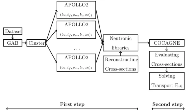
Dans la nouvelle chaîne de calcul ANDROMEDE, le code APOLLO2 développé au CEA est utilisé comme code réseau et le code COCAGNE développé à EDF-R&D est utilisé comme code de cœur. Actuellement, l’interpolation multilinéaire est utilisée pour la reconstruction des sections efficaces dans le code COCAGNE.

Pour le modèle d’interpolation multilinéaire, les sections efficaces sont pré-calculées sur une grille tensorielle à partir de valeurs discrétisées sur les axes des paramètres. Toutes les valeurs pré-calculées par APOLLO2 sur cette grille sont ensuite stockées directement dans les bibliothèques neutroniques. Avec ce modèle, le nombre de calculs APOLLO2 ainsi que la taille des bibliothèques neutroniques sont de l’ordre de O(nd) si on suppose que les sections efficaces dépendent de d paramètres et que chaque paramètre est discrétisé par n points sur l’axe correspondant. Avec les contraintes industrielles imposées à EDF, ce modèle devient trop coûteux en mémoire et en temps de calcul pour des situations complexes à cause de l’augmentation rapide et exponentielle du nombre de points de calcul. Ces situations peuvent arriver, par exemple, dans le cas accidentel où de nouveaux paramètres s’ajoutent (température de l’eau, taille des lames d’eau) et/ou quand le domaine de calcul s’étend (avec des domaines de définition plus larges).

Afin de dépasser les limitations du modèle actuel, l’objectif de cette thèse est de développer un nouveau modèle de reconstruction des sections efficaces pour répondre aux exigences suivantes :

(i) Calculs hors ligne : utiliser moins de pré-calculs effectués par le code réseau APOLLO2,

(18)

(iii) Calculs en ligne : avoir une bonne précision (de l’ordre du pcm (10−5)) pour l’évaluation des sections efficaces.

Une autre contrainte est qu’un calcul APOLLO2 en un point donné (de l’espace de phase des paramètres) fournit toutes les valeurs des sections efficaces en même temps. La raison est que toutes ces sections efficaces dépendent du même flux neutronique calculé par APOLLO2 et ce flux est coûteux en temps de calcul. Par conséquence, la reconstruction de chaque section efficace doit être optimisée avec les autres afin de limiter le nombre de calculs APOLLO2.

Face à ce problème, nous avons étudié et proposé un modèle appelé la décomposition de Tucker. Ce modèle est basé sur le format de Tucker - une approximation de tenseur de faible rang. Pour une section efficace représentée comme une fonction multivariée, la décomposition de Tucker se réalise comme suit:

(i) Calculs hors ligne :

— Nous construisons dans chaque direction, des fonctions d’une variable dites fonctions de base tensorielle directionnelle grâce à des techniques comme la “matricization” et la décom-position de Karhunen-Loève. Ces techniques sont utilisées pour acquérir et reconstruire, direction par direction, l’information à partir de valeurs des sections efficaces précalculées par le code APOLLO2. Les fonctions de base tensorielle directionnelle sont parfois ap-pelées simplement fonctions de base. En pratique, ces fonctions sont construites à partir de vecteurs propres de la décomposition de Karhunen-Loève.

— La section efficace considérée est approchée par une combinaison linéaire des produits tensoriels des fonctions de base.

— Les coefficients de la combinaison dans la décomposition de Tucker sont déterminés par un système d’équations linéaires. Ce système dépend de points dans l’espace de phase des paramètres (sur ces points nous devons utiliser les calculs APOLLO2). Dans notre travail, nous proposons de choisir ces points par une technique basée sur un algorithme dit “glouton” qui sera détaillée dans ce manuscrit.

(ii) Calculs hors ligne : Nous stockons dans la bibliothèque neutronique les vecteurs qui représen-tent les valeurs des fonctions de base tensorielle directionnelle aux points de calcul présélec-tionnés et les coefficients dans la décomposition de Karhunen-Loève.

(iii) Calculs en ligne : Nous utilisons l’interpolation de Lagrange pour évaluer les fonctions de base en un point donné et finalement, évaluer les sections efficaces en n’importe quel point de l’espace de phase des paramètres par la décomposition de Tucker.

Nous avons testé et validé notre modèle sur deux domaines de calcul : le domaine dit standard (les valeurs des paramètres sont proches d’un point particulier dit point nominal, qui détermine le fonctionnement nominal du réacteur) et le domaine dit étendu où les domaines de définition des

(19)

paramètres sont éloignés par rapport au cas standard. Les résultats obtenus montrent la performance de notre méthode : alors que le nombre de calculs APOLLO2 et le stockage dans la bibliothèque neutronique sont significativement réduits dans les étapes hors lignes, la précision de notre modèle reste meilleure ou égale à l’interpolation multilinéaire dans l’étape en ligne. Le creusage (a posteriori et a priori) pour les coefficients dans la décomposition de Tucker permet de réduire encore le stockage, ainsi que le temps de calculs en ligne, tout en gardant une précision similaire à notre approche initiale.

Présentation des chapitres

Chapitre 1

Ce chapitre présente succinctement les concepts neutroniques (réactions en chaîne, sections effi-caces, flux neutronique, équation du transport des neutrons,...) ainsi que le contexte de la simulation (structure multi-échelles du cœur d’un réacteur, schéma de calcul en deux étapes,...). L’objectif prin-cipal est d’aider le lecteur à mieux comprendre le contexte de notre travail.

Chapitre 2

Ce chapitre est dédié à décrire différents formats de tenseur de faible rang, tel que : format en r-termes, format en sous-espace tensoriel (le format de Tucker), format hiérarchique. Nous expliquons ensuite pourquoi nous avons choisi la décomposition de Tucker (basée sur le format de Tucker) pour le problème de reconstruction des sections efficaces.

Chapitre 3

Ce chapitre, basé sur notre premier article, détaille la méthode que nous proposons : la décom-position de Tucker. Les sections efficaces sont approchées par une combinaison linéaire des produits tensoriels des fonctions de base tensorielle directionnelle. Nous décrivons étape par étape les prob-lèmes suivants: la construction des fonctions de base tensorielle directionnelle (par une extension de la décomposition de Karhunen-Loève), la détermination des coefficients dans la combinaison (par un système d’équations linéaires en utilisant l’algorithme glouton). Un premier benchmark est aussi proposé pour comparer notre modèle avec l’interpolation multilinéaire.

Chapitre 4

Dans ce chapitre, basé sur notre deuxième article, nous proposons des benchmarks physiques sur les deux domaines de calcul : standard et étendu. Des analyses statistiques sont proposées qui nous permettent de déterminer les facteurs principaux pour améliorer la précision de la reconstruction

(20)

: augmenter le nombre de fonctions de base tensorielle directionnelle ou discrétiser plus finement certaines zones de valeurs des paramètres trouvées par l’analyse.

Chapitre 5

Ce chapitre, basé sur notre troisième article, présente la possibilité de creuser les coefficients dans la décomposition de Tucker. Deux techniques sont proposées : le creusage a posteriori et le creusage a priori. Le creusage a posteriori est effectué quand les coefficients sont déjà calculés et nous pouvons donc éliminer les plus petits coefficients. Le creusage a priori est basé sur une prédiction de valeurs des coefficients grâce à un ordre proposé pour les fonctions de base tensorielle directionnelle. Ces méthodes nous permettent de réduire significativement le nombre de coefficients pour une précision équivalente et ouvrent une possibilité de réduire le nombre de calculs APOLLO2.

Chapitre Conclusion

(21)

(22)

Introduction (English version)

Motivation

EDF is the first electricity utility in the world, thanks in particular to its nuclear power plants in France with 58 pressurized water reactors (PWR). In order to pilot and control the operation of these reactors, EDF has developed calculation chains that simulate the behavior of a reactor core. To face more and more exigent engineering demands in terms of calculation time and accuracy, a new core calculation chain, named ANDROMEDE, is being developed at EDF-R&D.

One of the elements of the chain is the neutron code, called COCAGNE, one goal of which is to solve numerically the neutron transport equation (or one of its approximations), which allows us to obtain physical quantities of interest to describe the behavior of the reactor, such as: the neutron flux, the effective multiplication factor, reactivity... The resolution of this equation requires a large amount of physical data, especially cross-sections.

In neutronics, cross-sections represent the interaction probability of an incident neutron with target nuclei, for different types of interaction. In a neutron simulation, the cross-sections can be represented as functions depending on several physical parameters. These parameters are used to describe the thermo-hydraulic conditions and the configuration of the reactor core, such as: fuel temperature, moderator density, boron concentration, xenon level, burnup,... Thus, the cross-sections are multivariate functions defined on a space called the parameters-phase space. The number of cross-section values in the simulation of a full core is in the order of several billion due to the core discretization in hundreds of thousands of cells, with different cross-section values in each cell.

In order to simulate the reactor core in a reasonable calculation time, an industrial calculation scheme consisting in the two following steps is used:

— Offline calculations: the cross-sections are pre-calculated by a code named lattice code on fixed and preselected points in the parameters-phase space. The neutron transport equa-tion is solved precisely through very fine spatial discretizaequa-tions on smaller patterns than the reactor core (typically a fuel assembly) and an energy discretization itself very fine (hun-dreds of groups). The neutron flux which is the output of this resolution is used for spatial

(23)

homogenization and energy condensation of cross-sections. The obtained information on cross-sections is stored in files, called neutron libraries.

— Online calculations: the cross-sections are evaluated at any point of the core by a core code and through an evaluation method based on the information stored in neutron libraries. These values are used as inputs for the resolution of the neutron transport equation at the reactor core level. The resolution is simplified on the full geometry, for example by using an approximation of diffusion. The core discretizations are much coarser than those used by the lattice code.

This scheme shows that between the two steps, a model of cross-section reconstruction is required to evaluate the cross-sections from pre-calculated and stored data in the neutron libraries. In the new calculation chain ANDROMEDE, the code APOLLO2 developed at CEA is used as lattice code and the core code COCAGNE developed at EDF-R&D is used as core code. Currently, multilinear interpolation is used for the reconstruction of cross-sections in the code COCAGNE .

For the multilinear interpolation model, cross-sections are pre-calculated on a tensorized grid from discretized values on the parameters axes. All pre-calculated values by APOLLO2 on this grid are then stored directly in neutron libraries. With this model, the number of APOLLO2 calculations and the size of neutron libraries are in the order of O(nd) if we assume that the cross-sections depend on d parameters and that each parameter is discretized by n points on the corresponding axis. With the industrial constraints imposed at EDF, this model becomes too expensive in memory and computation time for complex situations due to the rapid and exponential increase of calculation points. Such situations can happen, for example, in the incidental case where new parameters are added (water temperature, water blades) and/or when the calculation domain extends (with larger definition domains for the parameters).

In order to overcome the limitations of the current model, the aim of this thesis is to develop a new model of cross-sections reconstruction to respond to the following requirements:

(i) Offline calculations: use fewer pre-calculations performed by the lattice code APOLLO2. (ii) Offline calculations: store less data for the reconstruction of cross-sections and,

(iii) Online calculations: get a high accuracy (in the order of pcm (10−5)) for cross-section eval-uation.

Another constraint is that an APOLLO2 calculation at a given point (in the parameters-phase space) provides all the values of the cross-sections at the same time. The reason is that all these cross-sections depend on the same neutron flux computed by APOLLO2 and this flux is a time-consuming calculation. Therefore, the reconstruction of each cross-section must be optimized with the others in order to limit the number of APOLLO2 calculations.

(24)

Introduction (English version) 9

This is based on the Tucker format - a low-rank tensor approximation. For a cross-section represented as a multivariate function, Tucker decomposition is performed as follows:

(i) Offline calculations:

— We construct in each direction, the one-variate functions called tensor directional basis functions through techniques like the “matricization” and the Karhunen-Loève decompo-sition. These techniques are used to acquire and reconstruct, direction by direction, the information from cross-section values pre-calculated by APOLLO2. The tensor directional basis functions are sometimes simply called basis functions. In practice, these functions are constructed from eigenvectors of the Karhunen-Loève decomposition.

— The considered cross-section is approximated by a linear combination of tensor products of basis functions.

— The coefficients of the combination in the Tucker decomposition are determined by a system of linear equations. This system depends on points in the parameters-phase space (on these points we need to use APOLLO2 calculations). In our work, we propose to select these points with a technique based on an algorithm called “greedy” which will be detailed in this manuscript.

(ii) Offline calculations: We store in neutron libraries the vectors that represent the values of tensor directional basis functions at pre-selected calculation points, and the coefficients in the Karhunen-Loève decomposition.

(iii) Online calculations: We use the Lagrange interpolation to evaluate basis functions at a given point and finally, evaluate cross-sections at any point in the parameters-phase space by the Tucker decomposition.

We have tested and validated our model on two calculation domains: the domain named standard (parameters values are close to a particular point called nominal point, which determines the nominal operation of the reactor) and the domain called extended where definition domains of parameters are far from the standard case. The results obtained show the performance of our method: while the number of APOLLO2 calculations and storage in the neutron libraries are significantly reduced in the offline steps, the accuracy of our model is better or equal to multilinear interpolation in the online step. The sparse representation (a posteriori and a priori) for the coefficients in the Tucker decomposition allows us to further reduce storage, as well as the online calculation time, while maintaining a similar accuracy to our initial approach.

(25)

Presentation of chapters

Chapter 1

This chapter briefly presents neutron notions (reaction chain, cross-sections, neutron flux, neu-tron transport equation,...) as well as the simulation context (the multi-scale structure of the reactor core, the calculation scheme in two steps, ...). The main goal is to help readers reach a better un-derstanding of our problem.

Chapter 2

This chapter is dedicated to the description of different formats of low-rank tensors, such as: r-term format, subspace tensor format (Tucker format), hierarchical format. We then explain why we chose the Tucker decomposition (based on the Tucker format) for the cross-section reconstruction problem.

Chapter 3

This chapter, based on our first article, details our proposed model: the Tucker decomposition. The cross-sections are approached by a linear combination of the tensor products of the tensor directional basis functions. We describe step by step the following problems: the construction of tensor directional basis functions (by an extension of the Karhunen-Loève decomposition) and the determination of the coefficients in the combination (by a system of linear equations using the greedy algorithm). The first benchmark is also proposed to compare our model with the multilinear interpolation.

Chapter 4

In this chapter, based on our second article, we propose benchmarks on two calculation domains: standard and extended. Statistical analyzes are proposed that allow us to find the major factors to improve the reconstruction accuracy: increasing the number of tensor directional basis functions or discretizing finer some parameter values zones found by the analysis.

Chapter 5

This chapter, based on our third article, presents the possibility of a sparse representation of data (the coefficients in the Tucker decomposition) in our model. Two techniques are proposed: a posteriori sparse representation and a priori sparse representation. A posteriori sparse representa-tion is performed when the coefficients are already calculated and we can therefore remove small

(26)

Introduction (English version) 11

coefficients. A priori sparse representation uses a prediction of coefficients values based on an or-der proposed for tensor directional basis functions. These methods allow us to significantly reduce the number of coefficient for equivalent accuracy and open the possibility to reduce the number of APOLLO2 calculations.

Chapter Conclusion

(27)

(28)

Part I

Physical context and mathematical

background

(29)

(30)

Chapter 1

Physical context of the neutron

cross-section reconstruction

The purpose of this chapter is to present the physical context of neutron cross-section recon-struction. Some notions of neutronic physics related to our problem will be introduced. We refer the reader to the books [Lewis and Miller, 1984], [Reuss, 2003] and [Marguet, 2013] for more details of neutronic physics and nuclear reactors.

1.1 Nuclear reactions

1.1.1 Atomic structure and isotopes

We recall here some basic notions of the structure of an atom in order to get a better compre-hension for the next introduction. The atom is the unit component of matter, it consists of smaller particles (sub-atomic), such as: neutron (n), proton (p) and electron (e−) , as described in figure

1.1. The neutrons and the protons of an atom are called nucleons and they constitute the so-called a nucleus. The term nuclei is used to designate many nucleus. We often denote by the letter Z the number of protons and by the letter A the number of nucleons (protons and neutrons).

A chemical element is identified by the number Z. The isotopes (also called nuclide) of a chemical element are determined by an atom that has a fixed number of protons but different number of neutrons. For example, uranium has the following isotopes: uranium 234 (234₉₂ U ), uranium 235 (235₉₂ U ) and uranium 238 (238₉₂ U ), they have the same number of protons (92 protons) while the number of neutrons are respectively: 142, 143 and 146. Due to this difference, the isotopes of an element can have different properties, e.g: one can be fissible while others are not. An important property of fissile isotopes is to have uneven number of nucleons (A), e.g. 233₉₂ U , 235₉₂ U , 239₉₄ P u.

(31)

electron neutron proton atom(radius ∼ 10−8cm) nucleus (radius ∼ 10−12cm)

Figure 1.1 – Structure of an atom.

1.1.2 Principal reaction kinds

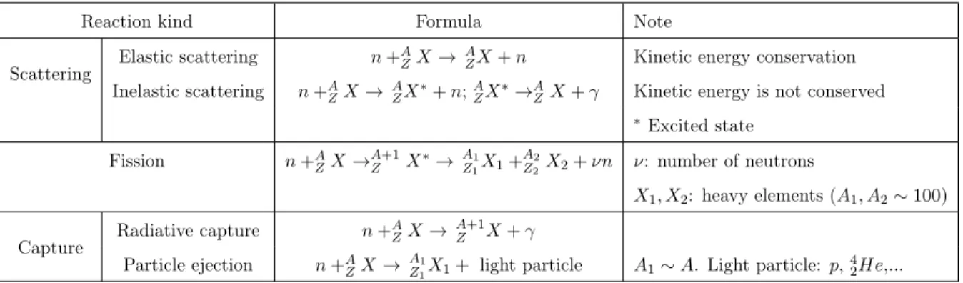
In table1.1, we present the principal reaction kinds of nuclear reactions: scattering, fission and capture.

Reaction kind Formula Note

Scattering

Elastic scattering n +A

ZX → AZX + n Kinetic energy conservation

Inelastic scattering n +A

ZX → AZX∗+ n;AZX∗→AZX + γ Kinetic energy is not conserved ∗_{Excited state} Fission n +A_ZX →A+1_Z X∗→A1 Z1X1+ A2 Z2 X2+ νn ν: number of neutrons X1, X2: heavy elements (A1, A2∼ 100) Capture Radiative capture n +A ZX → A+1 Z X + γ Particle ejection n +A ZX → A1

Z1X1+ light particle A1∼ A. Light particle: p,

4 2He,...

Table 1.1 – Principal reaction kinds of nuclear reactions.

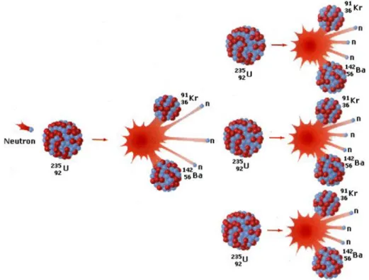
1.1.3 Nuclear fission chain reaction

A fission is a process in which a fissile nucleus (typically, Uranium U235

92 , Plutonium P u23994 )

absorbs neutrons and splits into lighter nuclei, for example:

235

92 U + n −→23692 U∗ −→9236Kr +14156 Ba + 3n (1.1)

This process produces new free neutrons (3 in example (1.1)) and releases a large amount of energy in the form of heat (about 200 MeV per fission of U235). Again, part of this newly produced free neutrons collide with other fissile nucleus (while the others can be absorbed by the non-fissile material or leak out of the material), which generates more heat, more neutrons and cause a reaction chain, see figure1.2.

The global behavior of the nuclear fission chain is related to a factor, called effective multiplication factor and denoted by k_{ef f}. The k_{ef f} is used to describe the average number of neutrons from one

(32)

1.1. Nuclear reactions 17

Figure 1.2 – Nuclear fission chain reaction.1

fission that cause other fissions. Therefore, this factor determines the evolution of the reaction chain, i.e. N fissions lead to the next ones: N k_{ef f}, N k2

ef f, N k3ef f, ..., fissions.

The value of kef f is classified as follows:

— kef f > 1 (super-criticality ): number of fissions increases exponentially and the reaction is

explosive.

— kef f = 1 (criticality): number of fissions is stable (constant) in time.

— kef f < 1 (sub-criticality): number of fissions decreases exponentially and finally the reaction

stops.

Fission rate (number of fissions per a unit time) depends on the population of neutrons. Thus, in order to reduce the number of neutrons which were born in the reactor core, absorbent substances (also called neutron poisons or neutron absorbers) are used, such as: boron, gadolinium, etc. The reaction chains themselves produce neutron poisons in their fission products, of which the most important substance is xenon-135 (135₅₄ Xe). The concentration of xenon increases quickly when the reactor starts (which may cause the reactor to shutdown at this stage) and gradually becomes more stable, see figure1.3.

The fission rate also depends on the energy E or the velocity v = ||−→v || of the incident neutron (since E = mv2/2). In general, the slow neutrons (corresponding to the low energy) are captured

(33)

Figure 1.3 – Xenon behavior in reactor core.2

more easily in the collision than the fast ones (corresponding to the high energy), meaning that the slow neutrons are more favorable for fission reactions. Therefore, a moderator medium which absorbs very few neutrons and slows down the fast neutrons is employed to increase the fission rate. A good moderator is regular water (H2O), a better one is heavy water (D2O).

1.2 Nuclear reactor

1.2.1 General description

A nuclear reactor is a system designed to initiate and control nuclear chain reactions. Depending on its purpose, it can be classified as the research reactor, the military reactor or the power reactor. Here, we are more interested in power reactors because they are used in the nuclear power plants to generate electricity.

The principal mechanism of nuclear reactors is that they produce thermal energy from the heat of nuclear chain reactions which is convert into mechanical or electrical form. Some important components in a nuclear reactor are:

— The core that contains nuclear fuels, control systems, and structural materials. The nuclear reactions take place inside the nuclear fuels and produce heat;

— The coolant that is a fluid circulating through the core and transferring the heat from the fuel to a turbine. It could be liquid (e.g. water), gas (e.g. hydrogen, helium), liquid gas (e.g. carbon dioxide);

— The turbine that converts the heat into electricity.

(34)

1.2. Nuclear reactor 19

1.2.2 Pressurised Water Reactors (PWR)

Pressurised Water Reactor (PWR) is the most widely used type of reactors for nuclear power plants in the world as well as in France. In a PWR, the heat is created by the fissions inside the fuels of the core. The core is put in a reactor vessel. Water (pressurized at about 155 atm to avoid boiling) circulates in a primary coolant loop and carries the heat (about 330˚C) to a steam generator. Inside the steam generator which has lower pressure, the water is vaporized and conducted through a secondary loop, spinning the turbine. The turbine is connected to a generator which produces electricity. The steam is then condensed back into water inside the condenser (figure 1.4). We note that between the primary and the secondary loop, there is only heat exchange but not water exchange. In the PWR core, water (used in the primary coolant loop) is also employed as moderator to slow down neutrons.

Figure 1.4 – Diagram of a pressurized water reactor.3

The PWR core has a multi-scale structure (figure1.5). It contains between 150-200 fuel assem-blies arranged as a square lattice and surrounded by boron water . A typical assembly is often made of 17 × 17 = 289 rods, consisting of 264 fuel rods and 25 vacant rods (figure 1.6a). The fuel rods (∼ 4 m in height) are filled with the individual pellets (∼ 1 cm in height) (see figure 1.6b). The vacant rods are dedicated for the vertical insertion of the absorbent rod in the guide tubes or the instrument.

(35)

Figure 1.5 – PWR - multi-scale structure: core containing many assemblies, assembly containing many rods.4

(a) Fuel assembly of PWR with about 289 rods.5

Fuel Rod (∼ 4 m)

pellet (∼ 1 cm )

(b) Fuel rod.

Figure 1.6 – Fuel assembly of PWR and fuel rod.

1.2.3 Some assembly types: UOX, MOX, UOX-Gd

As described in previous section, an assembly contains different fuels and vacant rods put in 289 positions. Depending on the fuel rod composition and position, we have different types of assemblies. We present here some assemblies related to our work.

4. Source of figure: Ph.D Thesis of Pierre GUÉRIN (Méthodes de décomposition de domaine pour la formulation mixte duale du problème critique de la diffusion des neutrons)

(36)

1.3. Neutronic 21

1.2.3.1 UOX (Uranium Oxide: U O2) assembly

Most reactors use uranium enriched in the isotope 235 with the enrichment is between 3%-5% because the natural uranium contains only 0.7% of uranium-235. The assembly constituted by the UOX fuel will be called the UOX assembly.

1.2.3.2 MOX (Mixed Oxide: U O₂-P uO₂ ) assembly

Plutonium (P u) is also a fissile source for nuclear reactors beside the natural uranium. It is produced inside the nuclear reactors by capturing the neutrons as the following reaction:

238 92 U + n −→23992 U −→23993 N p + e −_−→239 94 P u + e − (1.2)

Moreover, plutonium can be extracted from spent fuels. This allows us to recycle the used fuels. Therefore, MOX, an uranium fuel mixed with plutonium, is also used for the nuclear reactors. The assembly constituted by some MOX fuels will be called the MOX assembly.

1.2.3.3 UOX-Gd (UOX-Gadolinium: U O2-Gd2O3) assembly

An UOX-Gd assembly is an UOX assembly where some positions of the UOX fuel rods are replaced by U O₂-Gd₂O3 rods (gadolinia rods), see figure 1.7. Since the gadolinium Gd2O3 is a

neutron poison (absorbing neutrons), the U O₂-Gd₂O3 rods are used as burnable poison rods to limit

excess of fissions, hence to mitigate localized power peaking.

Guide Tube U O2 rod

(a) UOX assembly.

Guide Tube U O2 rod

gadolina rod

(b) UOX-Gd assembly.

Figure 1.7 – UOX and UOX-Gd assemblies.

1.3 Neutronic

1.3.1 Neutron cross-section

In order to quantify the neutron reaction rates, a notion which represents interaction probability between an incident neutron and a target nucleus or nuclei is required. This notion is referred to

(37)

as cross-section in particle physics. A simple explanation of cross-section notion is illustrated by figure1.8. In this figure, an incident neutron moves with a velocity −→v toward a target nucleus. The incident neutron and the target nucleus are supposed to have spherical forms with the radius r and R respectively. In this figure, a collision only happens if the mass center of the incident neutron is inside the cylinder of the radius R + r and of axis paralleling to the velocity −→v . Thus, the surface (or the cross-section) perpendicular to the axis of the cylinder represents the interaction likelihood of the incident neutron and the target nucleus. Neutron cross-section notion are therefore illustrated by the area of this surface. This explains why magnitude’s neutron cross-sections is in the order of 10−24cm2 (since the area ∼ πR2 and R ∼ 10−12cm). Cross-sections are measured in the unit barn:

1 barn = 10−24cm2= 10−28m2 Incident Neutron r∼ 10−13cm Target Nucleus R∼ 10−12cm − →_v R+r Cross Section σ

Figure 1.8 – Illustration for cross-section notion.

A cross-section may be microscopic, denoted by σ, that characterizes an individual target nucleus, or macroscopic, denoted by Σ, that describes the material interaction characteristic with a large number of target nuclei. Microscopic cross-sections depend on energy E of the incident neutron: σ = σ(E) whereas macroscopic cross-sections depend on spatial position −→r = −→r (x, y, z), energy E of the incident neutron at a given instant t: Σ = Σ(−→r , E, t). The relation between the macroscopic and microscopic cross-sections is defined by:

Σ(−→r , E, t) = N (−→r , t)σ(E)

where N (−→r , t) is the density of the target nucleus per a volume unit at the moment t. This relation implies that macroscopic cross-sections are expressed in inverse of length unit: [Σ] = cm−1.

The different cross-sections kinds are distinguished by their corresponding reaction which are denoted by the index r in (σ_r, Σr). Here, r could be: f (fission), s (scattering), c (capture), a

(38)

1.3. Neutronic 23

(absorption), t (total), ... The relations between these cross-sections are defined as follows:

σa= σf + σc; Σa= Σf + Σc

σt= σs+ σa; Σt= Σs+ Σa

Using the definition of the cross-sections, we deduce that the larger the cross-section is, the more likely interaction between the nucleus and the incident neutron is. Moreover, cross-sections depend on the isotope type. For example, at low neutron energy, the fissile isotope U₉₂235 has a large fission cross-section (σ_f, Σf) while for the isotope U92239 this cross-section is small.

Until now, we considered only cross-sections for an isotope kind i. In reality, most material is composite. Therefore, we need to determine a notion corresponding to the global macroscopic cross-section for the composite material. With a given reaction kind r, this macroscopic cross-cross-section is the sum of the macroscopic cross-sections of all elements:

Σr=Σr,1+ . . . + Σr,I =c1σr,1+ . . . + cIσr,I = I X i=1 ciσr,i (1.3)

where I is the number of isotopes i included in the composite material and ci is the concentration

of the isotope i.

1.3.2 Neutron flux

Cross-sections provide us information about interaction probability but this is not sufficient for studying the chain reactions. We also need information about the population of free neutrons in the medium inside a nuclear reactor. This population is sufficiently large (∼ 108 neutrons/cm3) to use the “neutron density” concept for simulating the variation of this population. Neutron density, denoted by n, is the number of neutrons per time unit t and per volume unit of a phase space Ω . Here, the phase space Ω for a neutron of mass m is spanned by its spatial position −→r = (rx, ry, rz)

and its velocity −→v . In neutronic, we prefer to replace −→v by (E,−→Ω = − →_v v ) since E = 1 2mv 2 _with

v := ||−→v ||. The direction of motion −→Ω is called solid angle which is defined in a polar coordinate system by a polar angle θ and an azimuthal angle α, i.e. −→Ω =−→Ω (θ, α). Thus, we can denote the phase space Ω = Ω(−→r , E,−→Ω ) and the neutron density n = n(−→r , E,−→Ω , t). The neutron population is then represented by the so-called angular flux ψ with the following definition:

ψ(−→r , E,−→Ω , t) = n(−→r , E,−→Ω , t)v (1.4)

(39)

The integral of the angular flux over whole solid angle gives us the so-called scalar flux φ with the following definition:

φ(−→r , E, t) = Z

4π

ψ(−→r , E,−→Ω , t)d2Ω (1.5)

The formula (1.4) means that the angular flux ψ(−→r , E,−→Ω , t) takes into account only the neutrons having the energy E and moving in the fixed direction −→Ω . The scalar flux φ(−→r , E, t) in (1.5) takes into account all neutrons having the energy E and moving in any direction with the condition that they are in a same volume d3−→r .

It can be noticed that the notion of “flux” in neutronics is completely different from which of classical fluid mechanics. The equivalent would be current−→j = n−→v .

1.3.3 Neutron transport equation

The neutron transport equation is based on the Boltzmann equation. The Boltzmann equation is proposed by Ludwig Boltzmann [Boltzmann, 1970] to describe the statistical behavior of mono-atomic gas. The properties of the neutron population in a reactor core are similar to this gas since the neutron density is very low compared with that of atoms. Therefore, this equation can be applied to the neutron population (by neglecting the neutron-neutron and neutron-electron interactions), to predict the global variation of this population.

The neutron transport equation can be written under different forms: either integral or integral-differential. These two forms are mathematically equivalent but the integral-differential one is often used for deterministic methods (to which this work is related). The integral-differential transport equation is expressed as:

1 v ∂ψ(−→r , E,−→Ω , t) ∂t = − − → ∇.[−→Ω ψ(−→r , E,−→Ω , t)] − Σt(−→r , E, t)ψ(−→r , E, − → Ω , t) + Z ∞ 0 dE0 Z 4π d2Ω0Σs(−→r , E0→ E, − → Ω0→−→Ω , t)ψ(−→r , E0,−→Ω0, t) + 1 4π Z ∞ 0

dE0χ(E0 → E)νΣ_f(−→r , E0, t)φ(−→r , E0, t) + Sext(−→r , E,

− →

Ω , t) (1.6)

Where:

— −→∇. is the divergence operator.

— χ(E0 → E) is the energy distribution spectra. — Sext is the external source term.

In order to reach the critical stationary state (where time-dependence terms disappear in (1.6)), we introduce a parameter to balance the appearance and disappearance terms. This parameter is considered as the effective multiplication factor k_{ef f} (see the section 1.1.3) and determined as the

(40)

1.3. Neutronic 25

eigenvalue of the following equation: − → ∇.[−→Ω ψ(−→r , E,−→Ω )] + Σt(−→r , E)ψ(−→r , E, − → Ω ) = Z ∞ 0 dE0 Z 4π d2Ω0Σs(−→r , E0→ E, − → Ω0 →−→Ω )ψ(−→r , E0,−→Ω0) + 1 4πkeff Z ∞ 0

dE0χ(E0 → E)νΣ_f(−→r , E0)φ(−→r , E0) + Sext(−→r , E,

− →

Ω ) (1.7)

This equation requires inputs as different macroscopic cross-sections: Σt, νΣf, Σs and provides us

outputs as neutron flux ψ(−→r , E,−→Ω ) and kef f.

A simplified equation of the equation (1.7) is the diffusion equation:

−−→∇.[D(−→r , E)−→∇φ(−→r , E)] + [Σa(−→r , E) + Z Emax Emin Σs(−→r , E → E0)dE0]φ(−→r , E) = Z Emax Emin Σs(−→r , E0 → E)φ(−→r , E0)dE0+ χ(E) kef f Z Emax Emin ν(E0)Σf(r, E0)φ(−→r , E0)dE0 (1.8)

Where D is the diffusion coefficient.

With the two-group energy theory (the energy E is discretized into two groups g = 1 and g = 2), the diffusion equation (1.8) becomes the two-group diffusion equations:

     −D14φ1+ (Σ1a+ Σ1→2s )φ1 = νΣ1_fφ1+ νΣ2_fφ2 kef f + Σ2→1_s φ2 −D₂4φ₂+ (Σ2_a+ Σ2→1_s )φ2 = Σ1→2s φ1 (1.9)

1.3.4 Reactivity in the infinite medium with two-group diffusion theory

The k_{ef f} value is used to describe the behavior of nuclear reactors. In normal operating conditions of reactor, k_{ef f} is equal to 1 (criticality value). When k_{ef f} varies, a small deviation from the criticality value can result a significant change in reactor power. Therefore, for the practical purpose, the “reactivity” is more useful with the following definition:

reactivity = 1 − 1 kef f

(1.10)

We consider here a simplified configuration: reactor core is assumed as a homogeneous infinite medium and the 2 two-group diffusion equations (1.9) are solved over this medium. Using this hypothesis, the reactivity can be determined by an analytic formula which takes into account some macroscopic cross-sections.

The infinite medium means that all assemblies have the same configuration and they are infinitely arranged together. In this medium, neutrons can not leak out of the system and the effective

(41)

multiplication factor kef f becomes the infinite multiplication factor k∞: kef f = k∞. With the

two-group diffusion theory, we obtain the following analytic formula (see page 1172, 1173, 1221 of the book [Marguet, 2013]): reactivity = 1 − 1 k∞ , with k∞= νΣ1_f ∗ (Σ2 t − Σ2→2so ) + νΣ2f ∗ Σ1→2so (Σ1_t − Σ1→1 so ) ∗ (Σ2t − Σ2→2so ) − Σ1→2so ∗ Σ2→1so (1.11)

This formula takes into account some macroscopic cross-sections (not all), such as: the macro totale-Σg_t, the macro fission-Σg_f, the macro nu*fission-νΣg_f and the macro scattering-Σg→gso 0, where

the energy group g ∈ {1, 2}, g0 ∈ {1, 2} and the index o in Σso is the anisotropy order (order for

Legendre polynomial expansion for variable “angle”).

1.4 Reactor core simulation and process of cross-section

reconstruc-tion

In the following descriptions, the neutron transport equation is always considered in the station-ary state (time-independence). This equation is also called transport equation in this work.

1.4.1 Numerical methods

Solving the neutron transport equation plays a fundamental role in reactor core simulation. Deterministic methods [Lewis and Miller, 1984] are used to solve numerically this equation (often under the integral-differential form). There are six parameters involved in such resolutions: three for −

→_{r = (r}

x, ry, rz), two for

− →

Ω = (θ, α) and one for E. The resolution is based on some discretization techniques, for instance:

— For space −→r : spatial discretization with finite difference methods [LeVeque, 2007] or finite element methods [Madenci and Guven, 2015].

— For angle−→Ω : angular discretization with discrete ordinates methods SN, spherical harmonics

methods P_N [Abramowitz and Stegun, 1964], or simplified spherical harmonics methods SP_N [Pomraning, 1993], [McClarren, 2010].

— For energy E: energy discretization with multi-group formalism [Hébert, 2010], often ex-pressed as follows: E = [Emax, Emin] = [E0, E1] | {z } group g = 1 ∪ [E1, E2] | {z } group g = 2 ∪ . . . ∪ [E_G−1, EG] | {z } group g = G (1.12)

(the energy groups are indexed by the index g in the decreasing order of energy because neutron energy decreases in time when colliding with moderator (water).)

In figure1.9, we summarize the principal numerical methods for solving the neutron transport equation.

(42)

1.4. Reactor core simulation and process of cross-section reconstruction 27

Neutron Transport Equation

Integral-Differential Form

Deterministic methods: discretization

Angle: SN, PN, SPN

Space: Finite Difference/Element Energy:Multi group

Figure 1.9 – Numerical methods to solve the neutron transport equation.

1.4.2 Calculation scheme with two steps

The neutron transport equation is well understood nowadays but its numerical resolution for the full core simulation is still a challenge, due to the requirement of memory storage and computational time. Indeed, for a real geometry modeling of core (core in 3D), we need to solve the neutron transport equation with a huge number of unknowns (∼ O(109)).

To deal with this problem, a two-step calculation scheme is proposed in order to reduce com-plexity calculations and accomplish the core simulation. This scheme is based on the multi-scale structure of the reactor core: core containing assemblies, assembly containing rods/cells. Therefore, the two steps are separately performed by two codes: first, lattice code for all assembly types and then core code for the whole core, as described in figure 1.10.

First step Second step

(43)

These two steps are respectively named assembly calculation and core calculation with the fol-lowing goals:

— Assembly calculation: the lattice code solves the neutron transport equation on each assembly type. These assemblies are assumed in a 2D infinite medium. The resolution is performed on a very fine discretization for space −→r and for energy E. Finally, we obtain the angular neutron flux ψ(−→r , E,−→Ω ) which is used in the energy condensation and the spatial average for cross-sections: Σg_r(cella) := Σ g r(cella) = R − →_{r ∈cell} a R E∈g Σr(−→r , E)ψ(−→r , E, − → Ω )d−→r dE R − →_{r ∈cell} a R E∈g ψ(−→r , E,→−Ω )d−→r dE (1.13)

where r is the reaction kind, g is the energy group and cell_ais a cell in a spatial discretization of the assembly a. All these results are gathered inside hierarchical library files which are named neutron libraries.

— Core calculation: the core code solves a simplified neutron transport equation for the full core in 3D. This resolution needs cross-section values at any point in the core. However, we can not calculate on the fly these values due to its huge cardinal (∼ O(109)). We therefore replace required values by their interpolation values based on a reconstruction process. This reconstruction process relies on the pre-computed values of Σgr determined by (1.13).

We illustrate in figure1.11the two-step calculation scheme for the core simulation.

First step Second step

Lattice code (for 2D- assemblies )

Solving transport equation - very fine discretization for:

space and energy

ψ Neutronic libraries Containing Σgr: - spatial average - energy condensation Core code (for 3D-core) Solving transport equation Cross-section reconstruction

Figure 1.11 – Two-step calculation scheme for the core simulation.

It should be noted that averaged and condensed cross-sections in (1.13) use the angular flux as weight functions in order to preserve the global reaction rate τ between the two steps: τ = Σgr R − →_r R E∈g ψ =R − →_r R E∈g Σrψ.

(44)

1.4. Reactor core simulation and process of cross-section reconstruction 29

1.4.3 Reconstruction of cross-sections in each calculation step

Cross-section values are required in the whole core simulation but we only have a limited num-ber of these values pre-calculated on assemblies because the two-step calculation scheme is used. Therefore, the reconstruction of cross-sections needs to be performed in order to connect the two calculation steps. This process can be briefly described as follows:

(i) Offline: pre-computing cross-sections on assemblies by a lattice code.

(ii) Offline: storing information about these pre-computed values in neutron libraries. (iii) Online: using the stored information to evaluate cross-sections in the core.

In order to avoid the confusion between the reconstruction notion used in the offline and online step, we distinguish here the two sub-processes:

— Reconstructing cross-sections: this is done before storing reconstruction information in the neutron libraries. Such sub-process is only explicit in the case where we need to convert pre-computed cross-section values into equivalent reconstruction information. If all pre-pre-computed cross-section values are kept and stored, no convertation process is required and performed. — Evaluating cross-sections: this is done for any point in the core. This sub-process uses

reconstruction information in the previous sub-process to evaluate cross-sections by an inter-polation method.

We call in general these two sub-processes by the reconstruction of cross-sections.

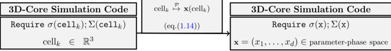
1.4.4 Reconstruction of cross-sections from 3D-space in the reactor core to parameter-phase space in the assemblies

In the nuclear reactor core simulations, cross-sections can be represented as multivariate func-tions: σ = σ(x₁, . . . , xd) and Σ = Σ(x1, . . . , xd), where d is the number of physical parameters on

which cross-sections depend.

Indeed, cross-sections depend on various parameters involved with different physical conditions and configurations, for instance: i) burnup-bu (M W d/t), ii) fuel temperature-t_f (˚C), iii) moderator density-ρ_m (g/cm3), iv) boron concentration-b_c (ppm), v) xenon level-xe (%), .... Here, the burnup parameter is used to measure how much the nuclear fuel is consumed, that is expressed by the fraction of the actual energy released per initial mass of fuel (gigawatt-days/ton). The other parameters (t_f, ρm, bc, xe) have already been introduced in previous sections. All these parameters vary in a physical

space named here parameter-phase space. (This is not the phase space presented in the section1.3.2

about neutron flux).

In the reactor core simulation, the core is modeled in 3D. Therefore, the core’s geometry is meshed by cells in a full three-dimensional coordinates Oxyz. In ordre to solve the transport