O
pen
A
rchive
T
OULOUSE
A
rchive
O
uverte (
OATAO
)
OATAO is an open access repository that collects the work of Toulouse researchers and
makes it freely available over the web where possible.
This is an author-deposited version published in :
http://oatao.univ-toulouse.fr/
Eprints ID : 13209
URL :
http://dx.doi.org/10.13140/2.1.4420.6885
To cite this version :
Benachir, Djaouad and Deville, Yannick and Hosseini,
Shahram and Karoui, Moussa and Hameurlain, Abdelkader Modified
Independent Component Analysis for Initializing Non-negative Matrix
Factorization :An approach to Hyperspectral Image Unmixing (2013) In:
WHISPERS 2013 : 5th IEEE Workshop on Hyperstectral Image and Signal
Processing : Evolution in Remote Sensing, 25 June 2013 - 28 June 2013
(Gainesville (Floride), United States).
Any correspondance concerning this service should be sent to the repository
administrator:
[email protected]
Modified Independent Component Analysis for
Initializing Non-negative Matrix Factorization:
An approach to Hyperspectral Image Unmixing
Djaouad Benachir∗‡§, Shahram Hosseini∗, Yannick Deville∗, Moussa Sofiane Karoui∗‡ Abdelkader Hameurlain§
∗IRAP, Université de Toulouse, UPS-OMP-CNRS, 14 av. Edouard Belin, 31400 Toulouse, France. {Djaouad.Benachir, Shahram.Hosseini, Yannick.Deville, Sofiane.Karoui} @irap.omp.eu
‡ASAL-CTS, Agence Spatiale Algérienne, Centre des Techniques Spatiales, Algeria. §IRIT, Université Paul Sabatier, 118 Route de Narbonne, 31062 Toulouse, France.
Abstract—Hyperspectral unmixing consists of identifying, from mixed pixel spectra, a set of pure constituent spectra (endmembers) in a scene and a set of abundance fractions for each pixel. Most linear blind source separation (BSS) techniques are based on Independent Component Analysis (ICA) or Non-Negative Matrix Factorization (NMF). Using only one of these techniques does not resolve the unmixing problem because of, respectively, the statistical dependence between the abundance fractions of the different constituents and the non-uniqueness of the NMF results. To overcome this issue, we propose an unsuper-vised unmixing approach called ModifICA-NMF (which stands for modified version of ICA followed by NMF). Consider the ideal case of a hyperspectral image combining (M − 1) statistically independent source images, and an Mth image depending on them due to the sum-to-one constraint. Our modified ICA first estimates these(M −1) sources and associated mixing coefficients, then derives the remaining source and coefficients, while it also removes the BSS scale indeterminacy. In real conditions, the above(M −1) sources may be somewhat dependent. Our modified ICA method then only yields approximate data. These are then used as the initial values of an NMF method, which refines them. Our tests show that this joint modifICA-NMF approach significantly outperforms the considered classical methods.
Keywords—ICA; NMF; hyperspectral unmixing.
I. INTRODUCTION
Remote sensing is the set of techniques used to determine, from a distance, object properties from the radiations they emit or reflect, depending on their molecular composition or shape. Historically, spatial remote sensing came to birth in the 1970s when different types of multispectral sensors emerged. Since then, these sensors have continued to improve up to the emergence of hyperspectral space sensors in the 2000s [1]. For each image pixel, the latter are capable to produce reflectance spectra in a large number of narrow and contiguous spectral bands. This allows the representation of a continuous spectrum, which is not the case of multispectral conventionally used sensors.
Nevertheless, due to the limited spatial resolution of most hyperspectral sensors, the pixel spectra composing the image are usually linear mixtures of elementary contributions from pure materials [2]. In such situations, traditional classification techniques are not acceptable for many major applications. It is therefore necessary to perform a Linear Spectral Unmixing (LSU). This procedure permits the decomposition of a mixed
pixel spectrum into a set of pure material spectra (endmembers) and a set of abundance fractions. A review of classical LSU methods may be found in [2]. Mathematically, LSU corresponds to the typical linear blind source separation (BSS) problem [3], where the collected pixels, endmember spectra and corresponding abundance fractions can be respectively considered as the observations, mixing matrix and sources. Most developed linear BSS methods are based on Independent Component Analysis (ICA) (see e.g. the review of classical methods in [3]). Under the source independence constraint, they provide a unique theoretical solution up to permutation and scale indeterminacies. However, the independence con-straint on sources is not met for remote sensing data [4]. When the sources and mixing matrix are non-negative, as in remote sensing images, methods relying on non-negativity constraints may be used. This especially includes methods based on non-negative matrix factorization (NMF). However, standard NMF methods are not guaranteed to provide a unique solution and their convergence point usually depends on their initialization [5]. In this paper, we propose an extended version of a new unsupervised unmixing approach, called modifICA-NMF [6], which combines a modified version of ICA with NMF. Our approach avoids the limitations which arise when using only one of the ICA and NMF methods. Indeed, we will show how the physical constraints of our problem can be used to eliminate indeterminacies related to ICA and to provide a first approximation of endmembers and abundance fractions. These approximations are then used to initialize NMF which provides refined estimates.
The remainder of the paper is organized as follows. In the second section, we present the data model. Section III de-scribes ICA and NMF methods and their limitations. Our proposed approach is presented in Section IV. In Section V, a comparative performance analysis for the proposed approach is provided, before concluding in Section VI.
II. DATA MODEL
We hereafter assume that each incident radiation interacts with a single type of material, which implies a linear mixing model [2]. In this case, the lth spectral component of thenth observed pixel can be expressed as follows:
xl(n) = M X
m=1
where:
• alm is the lth spectral component of the mth pure material,
• sm(n) represents the abundance fraction of the mth pure material in thenth pixel,
• M is the number of pure materials.
If one considers the N pixels of a hyperspectral image composed of L spectral bands, one gets the following matrix expression:
X = AS, (2)
where:
• X is the observed hyperspectral image, defined as: X = [x(1) · · · x(N )] with x(n) = [x1(n) · · · xL(n)] T
, • the columns ofA contain the endmember spectra:
A = [a1· · · aM] with am= [a1m· · · aLm] T
,
• each column ofS contains the abundance fractions of all pure components in the considered pixel:
S = [s(1) · · · s(N )] with s(n) = [s1(n) · · · sM(n)]T. Moreover, these data meet the following positivity and sum-to-one constraints: sm(n) ≥ 0, alm≥ 0 ∀ m = {1 · · · M } n = {1 · · · N } l = {1 · · · L} , (3) M X m=1 sm(n) = 1 ∀n = {1 · · · N } . (4) Using the BSS terminology, the abundance fraction matrix S and the endmember spectra matrix A will be hereafter respectively called source and mixing matrices. We aim at estimating the matrices S and A from an observation matrix X, representing the hyperspectral image.
III. LIMITATIONS OF STANDARDICAANDNMF When observations are linear combinations of statistically independent sources, ICA may be used to achieve BSS [3]. In our study, ICA cannot be applied in a standard manner to extract the M sources because they are statistically dependent due to the sum-to-one constraint (4) [4]. Besides, because of the scale indeterminacy inherent to ICA, the estimated abundance fractions provided by standard ICA are not physically interpretable. Nevertheless, we will show hereafter that a non-conventional use of ICA here yields approximations of source signals and mixing matrix without scale indeterminacy.
NMF [5] aims at deriving, from an observation matrix X consisting of non-negative elements, two other non-negative matrices ˆA and ˆS, such that:
X ≈ ˆA ˆS , X ∈ R+L×N, ˆA ∈ R+L×M, ˆS ∈ R+M ×N. Most NMF algorithms minimize an objective function by updating the estimated components ˆA and ˆS. The objective
function used in our investigation is the Euclidean distance defined by the following Frobenius norm:
DF = X −A ˆˆS F.
This function is minimized using the following Lee and Seung’s multiplicative update rules [7], [5]:
ˆ S ← ˆS ⊙ AˆT X ˆ ATA ˆˆS and A ← ˆˆ A ⊙ X ˆST ˆ A ˆS ˆST,
whereA⊙B and A
B respectively represent element-wise matrix multiplication and division.
The most important drawback of NMF is the non-uniqueness of this decomposition. It is well known that the convergence point of NMF algorithms highly depends on initialization. A random initialization of unconstrained NMF generally leads to a spurious solution. To obtain accurate matrix estimates, several methods make use of additional hypotheses about the sources and/or the mixing coefficients, particularly sparsity constraints [5], or of geometric constraints as in the MVC-NMF method [8]. In the next section, we propose an alternative approach to provide a suitable initialization of NMF.
IV. MODIFICA-NMFAPPROACH
The above discussion shows that the considered problem cannot be solved using only one of the ICA and NMF methods. We therefore propose a new approach consisting of the following 3 stages: (i) standard ICA is first used to provide approximations of (M − 1) sources and part of the mixing matrix up to some indeterminacies, (ii) indeterminacies are removed and approximations of the Mth source and the Mth column of the mixing matrix are computed. These first two stages will be hereafter considered as our modified ICA (modifICA). (iii) TheM estimated sources and the estimate of the mixing matrix are then used to initialize an NMF method. Thus, our approach consists in avoiding the non-uniqueness issue of NMF by initializing it with the result of a non-conventional extension of ICA.
A. First stage: ICA with(M − 1) components
As explained in Section III, because of the sum-to-one constraint (4), among all consideredM sources, only (M − 1) may be linearly independent. In practice, these(M −1) sources only have limited statistical dependence in various realistic scenarios: e.g. consider natural scenes, where(M − 1) classes of vegetation have moderately dependent spatial distributions, and the remainder of the scene (Mth class) consists of bare ground. In the first stage of our approach, we therefore use ICA to extract(M −1) independent components which provide first approximations of(M − 1) sources, to be refined in the next stages. More precisely, due to (4), and omitting the pixel indexn, Eq. (1) yields:
xl = al1s1+...+al(M −1)sM −1+alM(1 − ( M −1
X
m=1 sm)) = (al1−alM)s1+...+(al(M −1)−alM)sM −1+alM.(5) Modeling of linear mixture as in (5) has already been consid-ered in [9] but the authors do not explain how to reconstruct the actual sources and mixing matrix from this model.
Letα1, · · · , αM −1be(M − 1) arbitrary scale factors. Eq. (5) can then be rewritten as:
xl= al1−alM α1 α1s1+· · ·+ al(M −1)− alM αM −1 αM −1sM −1+a lM. (6) In the following, we denote the zero-mean versions ofxland smbyx¯l= xl− µxl ands¯m= sm−µsm, whereµxl andµsm
represent the means of xl andsm. Eq. (6) yields: ¯ xl= al1−a lM α1 α1¯s1+...+ al(M −1)− alM αM −1 αM −1¯sM −1. (7) Due to indeterminacies, when applying ICA to extract(M −1) components from allx¯l, we ideally get the mixing coefficient differencesali− alM and the zero-mean sources¯sm up to the above-defined unknown scale factors, i.e. we ideally obtain at the output of an ICA algorithm (with arbitrary source numbering): A∗ = a11−a1M α1 · · · a1(M −1)−a1M αM−1 .. . ... aL1−aLM α1 · · · aL(M −1)−aLM αM−1 and S∗ = α1¯s1 .. . αM −1¯sM −1 . (8)
B. Second stage: removing indeterminacies
The physical constraints of our configuration then allow us to eliminate indeterminacies related to ICA, as follows. We initially only consider the first (M −1) sources, involved in (8). The corresponding scale factors αm may be easily estimated if there exist at least one pure pixel for each of the M pure materials in the studied data (the procedure proposed below does not require one to know where the pure pixels are in the observed images). In this case, in each pure pixel, the abundance fraction of one of the materials is equal to one while the abundance fractions of all other materials are equal to zero. Thus, the actual sources satisfy the following conditions:
min{sm(n)} = 0 , max{sm(n)} = 1 , ∀m = 1, · · · , M . Considering (8) and denoting s∗
m(n) = αm(sm(n) − µsm),
we study the following two cases, separately for each source with indexm ∈ {1, . . . , M − 1}.
(1) The scale factorαm is positive. In this case: max{s∗ m(n)} = αm[max{sm(n)} − µsm] = αm(1 − µsm) min{s∗ m(n)} = αm[min{sm(n)} − µsm] = −αmµsm, which yields: αm= max{s∗m(n)} − min{s ∗ m(n)} (9) µsm = − min{s ∗ m(n)}/αm. (10) Knowing these values, we can find themthactual(i.e. without scale and mean-value indeterminacies) source:
sm(n) = s∗ m(n) αm + µsm= s∗ m(n) − min{s∗m(n)} max{s∗ m(n)} − min{s∗m(n)} . (11) (2) The scale factorαm is negative. In this case:
max{s∗ m(n)} = αm[min{sm(n)} − µsm] = −αmµsm min{s∗ m(n)} = αm[max{sm(n)} − µsm] = αm(1 − µsm), which yields: αm= min{s∗m(n)} − max{s ∗ m(n)} (12) µsm= − max{s ∗ m(n)}/αm, (13) and sm(n) = s∗ m(n) αm + µsm = s∗ m(n) − max{s ∗ m(n)} min{s∗ m(n)} − max{s∗m(n)} = 1 − s ∗ m(n) − min{s ∗ m(n)} max{s∗ m(n)} − min{s∗m(n)} . (14) In practice, the sign of the scale factor αm for each source is unknown. Hence, we do not know which of the equations (11) or (14) (respectively (9) or (12)) must be used to compute the actual source sm(n) (respectively the scale factor αm). Comparing Equations (11) and (14), it is clear that if the wrong equation is used, we obtain the inverted source: the zero-values in the actual source correspond to the one-values in the computed inverted source and vice versa. Let’s denote bys˜m(n) and ˜αm themth reconstructed source and the corresponding scale factor, computed using one of the couple of equations (9)-(11) or (12)-(14). If the right equations are used ˜sm(n) = sm(n) and ˜αm= αm, otherwise ˜
sm(n) = 1 − sm(n) and ˜αm= −αm.
In the following, we propose two strategies to solve the above problem, called sign indeterminacy in the BSS terminology.
First strategy: Each of the (M − 1) reconstructed sources ˜
sm(n) may be computed in two possible manners using (11) or (14). Thus, there are 2M −1 possible combinations for all (M −1) sources. For each of these combinations and all pixels with indexn, we compute the following criterion:
Q(n) = 1 − M −1 X m=1 ˜ sm(n). (15)
As shown in Appendix A, if all (M − 1) reconstructed sources are computed using the right equation, this criterion is non-negative ∀n. Otherwise, i.e. if at least one reconstructed source is computed using the wrong equation, the criterion becomes negative (and lower than or equal to -1) for at least a value of n if M > 2. This property can then be used to choose the right sources (and the corresponding factors αm) among all 2M −1 possibilities, when there are at least 3 endmembers in the hyperspectral image1.
Second strategy: In many applications, the number of pure pixels for each material is much lower than the number of pixels where that material is not present. Thus, we know that the number of zeros is higher than the number of ones for each actual source. If this is not the case after computing themthreconstructed source supposing a positive scale factor and therefore using Eq. (11), we deduce that the actual scale factor is negative and use Eq. (12) and (14) to compute αm
1Note that if only two endmembers are present in the whole image, ICA
is useless because in this case, due to the sum-to-one constraint, there is only one independent component.
and sm(n). In the simulations presented in Section V, the second strategy is used.
Once the first (M − 1) actual sources were found using the above procedure, theMth source may be computed using the sum-to-one constraint (4) by:
sM(n) = 1 − ( M −1
X
m=1
sm(n)). (16) Moreover, multiplying the mth column ofA∗ by the above-computed scale factor αm yields:
a11−a1M · · · a1(M −1)−a1M .. . ... aL1−aLM · · · aL(M −1)−aLM . (17)
Using the mean of (5), we can compute the entriesalM of the Mth column of the actual mixing matrixA as follows: alM = µxl − (al1− alM)µs1− · · · − (al(M −1)− alM)µsM−1.
(18) KnowingalMand matrix (17), we can finally deduce the actual mixing matrix, including theMth column:
A = a11 a12 · · · a1M .. . ... ... aL1 aL2 · · · aLM . (19)
C. Third stage: NMF initialization and update
The above method leads to perfect results in ideal con-ditions. In practice, however, the (M − 1) sources usually may be moderately statistically dependent. Besides, no ICA algorithm provides a perfect separation. Finally, the existence of a pure pixel per material may not be realistic in some configurations and data may be noisy. In such conditions, the source and mixing matrix estimates found by our modified ICA method may be unacceptable but they provide a rough approximation of the actual sources and mixing matrix. These approximate data may then be used to initialize an NMF algorithm subject to the sum-to-one constraint, which should provide better results.
In order to satisfy the sum-to-one constraint defined by (4) in the NMF update rule, we add to the observation and spectra matrices, a row consisting of a positive constant value [10].
V. EXPERIMENTAL RESULTS
In this section, we use the following normalized root mean square error to compare the estimated and actual abundance fractions (sources) as well as the estimated and actual spectra (mixing matrices):
N RM SE= kactual − estimatedk
kactualk . (20)
We also use the spectral angle mapper (SAM, in degrees) to compare the estimated and actual spectra:
SAM= arccos( hactual, estimatedi
kactualk · kestimatedk). (21)
In these equations, kxk and hx, yi respectively stand for the 2-norm ofx and the scalar product of x and y.
In a first experiment, we tested our method in an ideal case with (M − 1) independent sources. Thus, we first generated (M − 1) independent random abundance fraction maps, each one containing 6400 samples, uniformly distributed on [0,M1]. Then, we created an M
thsource using the sum-to-one constraint (4). We added to these data one pure pixel per source, i.e. a pixel where one of the sources is equal to one and all the others are zero. Finally, we mixed these M sources with a real-world mixing matrix containing M 420-point endmember spectra, randomly selected from the USGS spectral library [11]. We then applied our method for separating these mixtures.
TABLE I. RESULTS WITHM = 6ARTIFICIAL SOURCES
modif ICA modif ICA − N M F Spectra
N RM SE 0.022 0.012
SAM 0.85 0.50
Abundances
N RM SE 0.030 0.016
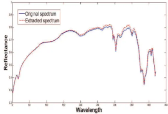
Table. 1 shows the average (over all sources) of NRMSE and SAM obtained using only modifICA or using NMF initialized by the outputs of modifICA (modifICA-NMF) for M = 6 sources. Our modified ICA provides very good results which are further improved by NMF. In Fig. 1, we present one of the spectra and its estimate using modifICA-NMF in this experiment. Fig. 2 illustrates the performance criteria for modifICA-NMF as functions of the number of sourcesM .
Fig. 1. Example of actual and estimated spectra used in the first test In another experiment,8 realistic sources (400 × 400-pixel abundance maps) were created from a real classification of land cover (see [12] for details). Contrary to the first experiment, these realistic sources, shown in Fig. 3, are moderately depen-dent. The observed hyperspectral images were then generated according to the linear mixing model described in Eq. (2), by mixing these sources using eight 431-point spectra from the AGC spectral library [13].
The RGB composition of the observations is shown in Fig. 4. The estimated abundance fraction maps using only the modifICA part of our approach and using the entire modifICA-NMF approach are respectively shown in Fig. 5
Fig. 2. Performance criteria vs. number of sources
Fig. 3. The eight sources used in the second test (the white color represents the one-values).
Fig. 4. RGB composition of the observed hyperspectral image
Fig. 5. The approximations of the sources derived by ModifICA.
and 6. The results obtained by modifICA are not acceptable for some of the maps (e.g. the first one in Fig. 5) because the independence assumption is not totally verified. However, the entire modifICA-NMF approach provides very good results which are similar to the actual maps (Fig. 6).
Fig. 6. The eight sources estimated by ModifICA-NMF. TABLE II. RESULTS WITH REALISTIC SOURCES
N M F M V C − N M F modif ICA − N M F Spectra N RM SE 0.120 0.103 0.029 SAM 4.83 4.88 1.22 Abundances N RM SE 0.131 0.098 0.003
Table. 2 shows the results obtained using standard NMF and MVC-NMF (presented in [8]) methods with a random initialization and our modifICA-NMF method. These results confirm the good performance of our algorithm in a realistic configuration as compared to these classical methods. In Fig. 7, we present one of the actual spectra and its estimate using modifICA-NMF.
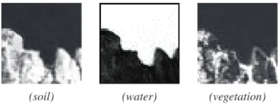
Fig. 7. Example of actual and estimated spectra used in the second test. Finally, we applied our approach to a(50 × 50) subimage from the Moffett Field (CA, in 1997) acquired by the AVIRIS spectro-imager. This subimage is mainly composed of three components: water, soil, and vegetation [14]. In Fig. 8, we present the 3 abundance maps obtained with our algorithm. These results are visually similar to those reached by a more complex Bayesian method presented in [14], but we cannot compare both of them quantitatively to the lacking ground truth.
(soil) (water) (vegetation)
Fig. 8. The abundance fraction maps estimated by the proposed approach
It is worth mentioning that all our reported results have been obtained using the kurtosis-based FastICA algorithm [3], which relies on the non-Gaussianity of source signals. How-ever, other tests of the proposed approach were also undertaken using other ICA methods such as JADE [3] yielding the same results as with FastICA.
VI. CONCLUSION AND FUTURE WORK
In this paper, a new unsupervised unmixing approach for hyperspectral images was proposed. It is based on two broad classes of BSS methods. We first modified standard ICA taking into account the sum-to-one constraint and then eliminated some indeterminacies related to ICA using different strategies. The obtained outputs were then used to initialize an NMF method which refines them. The efficiency of our approach was experimentally validated, first in an ideal configuration involving artificial sources, then using realistic simulated data and finally using real data (without ground truth). The test results thus obtained show the attractiveness of using our modified ICA as a pre-processing stage for NMF, compara-tively to classical methods. This motivates us to continue this work by determining the performance of our method for other abundance fraction maps mixed with other spectra, and for other real recorded hyperspectral images.
APPENDIXA
Among the first (M −1) sources involved in (8), suppose K reconstructed sourcess˜m(n) (corresponding to a first set D1) are computed using the wrong formula and the(M − 1 − K) others (represented by a second set D2) are reconstructed by the right one. There are 3 possible cases:
(1) K = 0, i.e. all the sources are correctly reconstructed. In this case the criterion (15) yields:
Q(n) = 1 − M −1
X
m=1
sm(n) = sM(n) (22) which corresponds to the Mth actual abundance fraction whose value is between 0 and 1.
(2) 1 ≤ K ≤ M − 2, such that D1 and D2 each contain at least one source. The criterion (15) becomes in this case:
Q(n) = 1 − X i∈D1 (1 − si(n)) − X j∈D2 sj(n) = 1 − K + X i∈D1 si(n) − X j∈D2 sj(n). (23) In a pure pixel n corresponding to one of the sources in D2, the value of that source is equal to one while all the other sources are zero. Thus, from (23),Q(n) = −K ≤ −1 in that pixel.
(3)K = M − 1, such that all the sources are inverted. In this case: Q(n) = 1 − M −1 X i=1 (1 − si(n)) = 1 − (M − 1) + M −1 X i=1 si(n) = 2 − M + (1 − sM(n)) = 3 − M − sM(n). In a pure pixel where sM(n) = 1, the criterion becomes Q(n) = 2 − M ≤ −1 if M > 2.
ACKNOWLEDGMENT
We would like to thank D. Ducrot and A. Halimi for providing us with remote sensing images used in some of our tests. This work was partly supported by "Axe transverse anal-yse et traitement de données" of Observatoire Midi-Pyrénées (Toulouse, France).
REFERENCES
[1] G. Shaw and D. Manolakis, “Signal processing for hyperspectral image exploitation,” in Signal Processing Magazine. IEEE, 2002, vol. 19, Issue 1, pp. 12–16.
[2] J.M. Bioucas-Dias, A. Plaza, N. Dobigeon, M. Parente, Q. Du, P. Gader, and J. Chanussot, “Hyperspectral unmixing overview: Geometrical, statistical, and sparse regression-based approaches,” in IEEE J. of Sel. Topics in Appl. Earth Observ. Remote Sens., 2012, vol. 5, no. 2, pp. 354–379.
[3] A. Hyvärinen, J. Karhunen, and E. Oja, “Independent component analysis,” John Wiley and Sons, 2001.
[4] J.M.P. Nascimento and J.M. Bioucas-Dias, “Does independent compo-nent analysis play a role in unmixing hyperspectral data?,” in IEEE Trans. on Geosci. and Remote Sensing, 2005, vol. 43, no. 1, pp. 175– 187.
[5] A. Cichocki, R. Zdunek, A. H. Phan, and S-I. Amari, “Nonnegative matrix and tensor factorizations: Applications to exploratory multi-way data analysis and blind source separation,” John Wiley and Sons, 2009. [6] D. Benachir, Y. Deville, S. Hosseini, M.S. Karoui, and A. Hameurlain, “Hyperspectral image unmixing by non-negative matrix factorization initialized with modified independent component analysis,” in Proceed-ings of the fifth IEEE Workshop on Hypers. Image and Signal Proces.: Evolution in Remote Sensing (WHISPERS), Gainesville, USA, 2013. [7] D.D. Lee and H.S. Seung, “Algorithms for non-negative matrix
factorization,” in Advances in Neural Information Processing Systems, 2001, vol. 13, pp. 556–562.
[8] L. Miao and H. Qi, “Endmember extraction from highly mixed data using minimum volume constrained nonnegative matrix factorization,” in IEEE Trans. on Geosci. and Remote Sensing, 2007, vol. 45, no. 3, pp. 765–777.
[9] C-Y. Kuan and G. Healey, “Using source separation methods for end-member selection,” in SPIE. Algorithms and Technologies for Multispectral, Hyperspectral, and Ultraspectral Imagery VIII, 2002, vol. 4725, pp. 10–17.
[10] D.C. Heinz and C.I. Chang, “Fully constrained least squares linear spec-tral mixture analysis method for material quantification in hyperspecspec-tral imagery,” in IEEE Trans. on Geosci. and Remote Sensing, 2001, vol. 39, no. 3, pp. 529–545.
[11] R. N. Clark, G. A. Swayze, R. Wise, E. Livo, T. Hoefen, R. Kokaly, and S. J. Sutley, “USGS digital spectral library splib06a,” in U.S. Geological Survey, Digital Data Series 231, http://speclab.cr.usgs.gov/spectral.lib06, 2007.
[12] M.S. Karoui, Y. Deville, S. Hosseini, and A. Ouamri, “Blind spatial unmixing of multispectral images: New methods combining sparse component analysis, clustering and non-negativity constraints,” in Pattern Recognition, 2012, vol. 45, pp. 4263–4278.
[13] “http :// www.tec.army.mil/hypercube,” .
[14] O. Eches, N. Dobigeon, and J.-Y. Tourneret, “Enhancing hyperspectral image unmixing with spatial correlations,” in IEEE Trans. on Geosci. and Remote Sensing, 2011, vol. 49, issue 11, pp. 4239–4247.