An 1d-beam approach for both stress analysis and fatigue life prediction of bonded joints

Any correspondence concerning this service should be sent to the repository

administrator:

staff-oatao@listes-diff.inp-toulouse.fr

O

pen

A

rchive

T

oulouse

A

rchive

O

uverte (

OATAO

)

OATAO is an open access repository that collects the work of Toulouse researchers and

makes it freely available over the web where possible.

This is an author version published in:

http://oatao.univ-toulouse.fr/

Eprints ID: 17647

To cite this version:

Paroissien, Eric and Da Veiga, Anthony and Laborde, Audrey An

1d-beam approach for both stress analysis and fatigue life prediction of bonded joints.

(2011) In: 26th ICAF Symposium, 1 June 2011 - 3 June 2011 (Montréal, Canada).

AN 1D-BEAM APPROACH FOR BOTH

STRESS ANALYSIS AND FATIGUE

LIFE PREDICTION OF BONDED

JOINTS

E. Paroissien1, A. Da Veiga1 and A. Laborde1

1 _{SOGETI HIGH TECH, TRPE, PE6, Blagnac, France}

Abstract: An approach for both stress analysis and fatigue life prediction of bonded joints, based on a 1D-beam model, is presented. Only the adhesive is supposed to fail. The Goland and Reissner framework [1] is extended to unbalanced laminar or monolithic adherends under thermal loads. The J-integral is derived and employed in a modified Paris law, leading to fatigue lives, which are assessed w.r.t. published experimental results [2,

3]_.

INTRODUCTION

In the frame of the structural component design, bonding can be considered as a suitable assembly method or an attractive complement to conventional ones as mechanical fastening. Bonding offers the possibility of joining without damaging various materials, such as plastics or metals, as well as various combinations of materials. This first advantage is reinforced by a large choice of adhesive families and by the possibility to formulate adhesives to meet at best the joint specifications. Compared to bolting, bonding shall allow for mass benefits, since the continuous distribution of load transfer all over the overlap implies that additional concentrated materials are not required to sustain loads. Nevertheless, the main restriction to a more widespread application of bonding could be the lack of assessment ability of its reliability. To our knowledge, non destructive test methods allow for detecting possible adhesive absences but not the adhesion absences. As a result, to control the design of bonded joints, it is necessary to predict its strength, including both stress and fracture analyses. In this paper, a 1D-beam approach, allowing both for stress analysis and fatigue life prediction of

bonded joint, is presented. Only the adhesive is supposed to fail. The single-lap bonded joint described in [2] (see Figure 1) allows for exemplifying the approach. Firstly, a general 1D-beam model for bonded joint stress analysis is presented. The model can be related to the Goland and Reissner framework [1], which is extended by considering unbalanced overlaps made of laminated monolithic beams under thermal loading (thermal mismatch effect). The computation method [4], inspired by the finite element method (FEM), enables solving the full set of equations. It is based on the analytical formulation of macro-element with four nodes, called bonded-beams (BB) element, able to simulate an entire bonded overlap. The model provides the distribution in the adherends of normal displacements, deflections and bending angles and of normal forces, shear forces and bending moments, as well as the distribution of adhesive shear and peeling stresses along the overlap. Elements of validation are then presented, in order to show that same hypotheses lead to same results. Secondly, the presented approach is employed to predict fatigue life of bonded joints, through elementary manipulations consisting in the introduction of adhesive cracks at both overlap ends. A modified form of Paris law [2, 3] allows for linking the fatigue cycle crack growth rate and the maximum energy release rate per cycle. The maximum energy release rate is related to the computation of the J-integral, the analytical simplified expression of which is derived, based on [5-7], in the presented framework. The approach is assessed with regard to experimental fatigue test results on isotropic balanced single-lap bonded joints, provided in [2, 3]. A way to simply approximate the thermal mismatch effect is suggested and remains to be assessed.

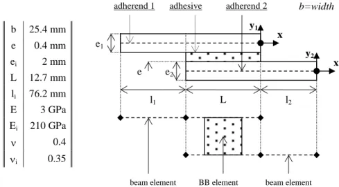
Figure 1 – Idealization of a single-lap bonded joint with of beam and BB elements. Geometrical and mechanical parameters [2]

b 25.4 mm e 0.4 mm ei 2 mm L 12.7 mm li 76.2 mm E 3 GPa Ei 210 GPa  0.4 i 0.35 adherend 1 BB element adhesive adherend 2 beam element beam element e1 e2 l1 L l2 e x y1 y2 x b=width

1D-BEAM MODEL FOR BONDED JOINT STRESS ANALYSIS

Overview of the approach [4]

The presented approach allows for the resolution of the set of differential equations. The bonded joint is meshed in elements (see Figure 1). While the parts outside the bonded overlap are simulated by beam elements, the bonded overlap is simulated by a four nodes macro-element, called bonded-beams (BB) element; this macro-element is the model core and is specially formulated. After finding the stiffness matrices of each element type, the stiffness matrix of the full structure – termed K – is assembled. The boundary conditions are then introduced. The vector of displacements – termed U – and the vector of forces – termed F – including the thermal equivalent nodal forces – termed FT – are determined; the stiffness matrix

is updated. The resolution consists then in inverting the linear system F=KU. Hypotheses

The model is based on the following hypotheses: (i) the thickness of the adhesive layer is constant along the overlap, (ii) the adherends are considered as linear elastic Euler-Bernoulli laminated or monolithic beams, (iii) the adhesive layer is simulated by a linear two-parameter uncoupled elastic foundation and consists thus in a continuously distributed layer of shear and transverse normal springs, (iv) the temperature is uniformly distributed on the adherends. In particular, the hypothesis (iii) implies that the adhesive stress field is reduced to the shear and peeling stress only, constant in the adhesive thickness. A quasi-static analysis is considered. Formulation of BB element

Governing equations. The subscript i refers to the ith adherend; i=1,2. Each adherend is associated to a local referential x, yi, zi (see Figure 1); the origin of

which is located at its neutral line; the neutral line is oriented according to an x-axis, while the y-axis is defined according to its thickness.

In the frame of the classical Euler-Bernoulli model of beams, the assumed displacement field is under the shape:

 

x,y w

 

x ' w ; y u dx dw y ) 0 , x ( u ) y , x ( ' u_{i j}  _i  _i i  _i _i_{i i j}  _i (1)

where ui’ and wi’ are the displacement of any points of the ith adherend

cross-section according to the x- and yi-axis, respectively; ui and wi are the displacement

of points located at the ith adherend neural line according to the x- and yi-axis,

respectively; i is the bending angle. By taking into account the thermal strain due

to a variation of temperature T, the tensile stress can be expressed as:

 

 

           ₂i _{i i T} 2 i i i i i y dx w d y dx du y E    (2) where Ei is the Young’s modulus and i the thermal expansion coefficient.

The integration on the cross-section of tensile stresses and elementary bending moments induced by these tensile stresses allows for the computation of the normal force Ni and bending moment Mi:









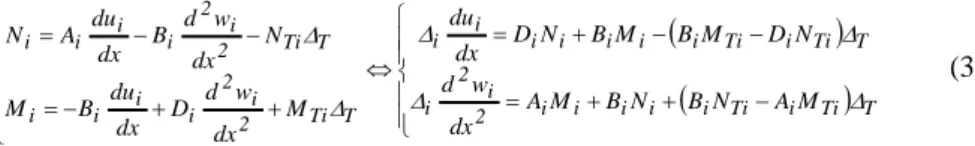
                             T Ti i Ti i i i i i 2 i 2 i T Ti i Ti i i i i i i i T Ti 2 i 2 i i i i T Ti 2 i 2 i i i i M A N B N B M A dx w d N D M B M B N D dx du M dx w d D dx du B M N dx w d B dx du A N       (3)

where Ai is the extensional stiffness, Di is the bending stiffness, Bi the extension

bending coupling stiffness, NTi is the thermal force per °K, and MTi is the bending

moment per °K, i=AiDi-Bi² 0.

The local equilibrium of adherends is performed according to [1] (see Figure 2):

 

 

bT 0 2 e V dx dM ; S 1 bdx dV ; T 1 bdx dN _i i i 1 i i i i _{   }  _{   (4)}

where b is the overlap width and Vi is the shear force.

Figure 2 – Free body diagrams of infinitesimal adherend elements of the overlap The adhesive shear stress T and the adhesive peeling stress S are then given by:



1 2



1 1 1 2 2 2 w w e E E S ; 2 e u 2 e u e G G T          _{  }       (5) N1(x+dx) V1(x+dx) M1(x+dx) V1(x) N1(x) M1(x) bdxT bdxS N2(x+dx) V2(x+dx) V2(x) N2(x) M2(x) bdxT bdxS M2(x+dx)

where G and E are the adhesive Coulomb’s and Young’s moduli. In the case of an enclosed adhesive layer, the effective Young’s modulus could be used instead of the Young’s modulus.

System of differential equations in terms of adhesive stresses. By combining Eqn. 3, Eqn. 4 and Eqn. 5, the following differential equation system is obtained in terms of adhesive stresses:

dx dT k S k dx S d ; S k dx dT k dx T d 3 4 4 4 2 1 3 3      (6)

where the constants are:

                                                                                2 2 1 1 2 2 2 1 1 1 3 2 2 1 1 2 2 2 1 1 1 2 2 2 1 1 4 2 2 2 1 1 1 2 2 2 2 2 2 1 2 1 1 1 1 1 B B 2 A e 2 A e e Eb k ; B B 2 A e 2 A e e Gb k A A e Eb k ; B e B e D 4 e A 1 D D 4 e A 1 D e Gb k               (7)

This system of differential equations in terms of adhesive stresses can be uncoupled by consecutive differentiations and combinations as:

                         0 ) ( 0 ) ( 4 1 3 2 2 2 4 4 4 1 6 6 4 1 3 2 2 2 4 4 4 1 6 6 k k k k T dx T d k dx T d k dx T d dx d k k k k S dx S d k dx S d k dx S d (8) The Cardan’s method is employed to solve the characteristic equation of the differential equation system in Eqn. 8 (see Appendix A) and find its root r² and (sit)² – r, s and t are positive real numbers – so that the adhesive shear and peeling stress are given by:

                                           7 6 5 4 3 2 1 6 5 4 3 2 1 ) cos( ) sin( ) cos( ) sin( ) ( ) cos( ) sin( ) cos( ) sin( ) ( K e K e K tx e K tx e K tx e K tx e K x T e K e K tx e K tx e K tx e K tx e K x S rx rx sx sx sx sx rx rx sx sx sx sx (9) Nodal displacements and forces. The computation of the BB element stiffness matrix takes place through the determination of nodal displacements and forces (see Figure 3). The second term of equivalency in Eqn. 3, together with Eqn. 4, allows uncoupling the expressions of derivatives of u1, u2, w1 and w2 (and then 1

and 2) as a function of linear combinations of adhesive stress derivatives and

polynomial expressions; following the resolution scheme in [8], the total number of independent integration constants can be reduced to 12:

                                                                                                  _           _{ }                        6 7 2 2 1 3 2 0 6 6 2 5 7 2 2 1 3 2 0 5 5 1 3 2 2 1 3 0 6 2 2 2 4 4 2 3 2 2 1 3 0 5 2 2 2 4 3 1 6 2 5 1 7 2 1 2 6 2 1 1 5 2 2 0 2 7 2 2 2 2 6 5 2 1 0 1 7 2 1 1 1 ~ K L J L x J 2 L x J 3 dx dS T ~ ) x ( ~ K L J L x J 2 L x J 3 dx dS T ~ ) x ( J L x J L x J L x J S dx S d k dx dT k ~ ) x ( w J L x J L x J L x J S dx S d k dx dT k ~ ) x ( w ~ 2 e ~ 2 e K ) e e ( L 2 J J L x ) e e ( L J J L x A 2 L J B 6 K bL dx dS T ~ ) x ( u J L x J L x A 2 L J B 6 K bL dx dS T ~ ) x ( u                   (10) with:

                             _                                       7 2 2 1 1 2 1 2 1 3 0 3 2 4 1 6 4 3 2 4 1 5 3 3 2 4 1 1 20 2 20 6 3 2 4 1 3 20 4 20 6 3 2 4 1 1 10 2 10 5 3 2 4 1 3 10 4 10 5 3 2 4 1 1 20 2 20 2 3 2 4 1 3 20 4 20 2 3 2 4 1 1 10 2 10 1 3 2 4 1 3 10 4 10 1 K A B A B 6 ) e e ( 3 A 1 A 1 bL J k k k k ~ ~ ; k k k k ~ ~ k k k k k B k A ; k k k k k B k A ~ k k k k k B k A ; k k k k k B k A ~ k k k k k D k C ; k k k k k D k C ~ k k k k k D k C ; k k k k k D k C ~            

















                              2 2 20 2 2 2 2 20 1 1 10 1 1 1 1 10 2 2 20 2 2 2 2 20 1 1 10 1 1 1 1 10 b B D ; D 2 B e 2 b C b B D ; D 2 B e 2 b C b A B ; A e B 2 2 b A b A B ; A e B 2 2 b A         (11)

The 12 nodal displacements are then the values at x=0 and x=L of the previous expressions of displacements, as a function of 12 integration constants. The relationship U=MC can be written in the form of a matrix, where C is the integration constant vector. By introducing Eqn. 10 in Eqn 3 and with Eqn. 4, the normal and shear forces and the bending moment in both adherends can be computed as a function of the 12 integration constants (Eqn. 12), leading to the expressions of nodal forces (see Figure 3), which can be written F=NC at T=0°K.

                                                                                                       T 2 b e A B bLK A L J 6 L 1 dx S d a dx T d a ~ ) x ( V T 2 b e A B bLK A L J 6 L 1 dx S d a dx T d a~ ) x ( V M L J B L e e B L D 2 J A B bLK A L J 6 L x dx S d a dx dT a ~ ) x ( M M L J B L J D 2 A B bLK A L J 6 L x dx S d a dx dT a ~ ) x ( M N L J A L e e A L B 2 J x bK dx S d a dx dT a ~ ) x ( N N L J A L J B 2 x bK dx S d a dx dT a ~ ) x ( N 2 2 2 7 2 2 2 0 3 3 4 2 2 4 2 1 1 1 7 1 1 2 0 3 3 3 2 2 3 1 T 2 T 5 2 2 2 1 2 2 2 1 2 2 7 2 2 2 0 2 2 4 4 2 T 1 T 5 1 2 1 1 1 1 7 1 1 2 0 2 2 3 3 1 T 2 T 5 2 2 2 1 2 2 2 1 7 2 2 2 2 2 T 1 T 5 1 2 1 1 7 2 2 1 1 1        

(12) with:

                            6 2 2 2 4 6 2 2 2 4 5 1 1 1 3 5 1 1 1 3 6 2 2 2 2 6 2 2 2 2 5 1 1 1 1 5 1 1 1 1 D B a ; ~ D ~ B a~ D B a ; ~ D ~ B a~ B A a ; ~ B ~ A a~ B A a ; ~ B ~ A a~                

(13)

Figure 3 – Bonded-beams element: a four-nodes macro-element with three degrees of freedom per node (u, w, )=i,j,k,l.

Stiffness matrix of BB element. The coefficients of the stiffness matrix are obtained by differentiating each nodal force by each nodal displacement. Of course, the stiffness matrix is not modified by the consideration of a thermal load:

0 K l , k , j , i , , S w S u S R w R u R Q w Q u Q K T BB BB _                                                                                                                          (14)

The twelve nodal displacements (u,  = 1:12) and the twelve nodal forces (Q,  = 1:12) are expressed as functions of the twelve independent integration constants (C,  = 1:12) at T=0°K. The nodal forces depend linearly on integration

constants as well as the nodal displacements. Thus, the integration constants depend linearly on the nodal displacements (Eqn. 15), enabling the determination of 144 coefficients of KBB (Eqn. 16): x y node i node j node k node l u2(x) u1(x) uk ul ui uj adhes w1(x) w2(x) wi wk wl wj i j k l 1(x) 2(x) e 0 x L x y node i node j node k node l N2(x) N1(x) Qk Ql Qi V1(x) V2(x) Ri Rk Rl Si Sk Sl M1(x) M2(x) e 0 x L Qj Rj Sj





    12 1 12 1 u ' m C and C n Q         (15)

 

_          u u ' m n u Q (16) But: ) 0 , , 0 , 1 u , 0 , 0 ( C ) 0 u , 1 u ( C ' m ' m n u Q if 0 if 1 u u 12 1                      



                    (17)

The coefficients of KBB are thus obtained through:





_

      12 1 , BB n C (0 0,u 1,0 0) u Q K           (18) Practically, C_(0…0,u_=1,0…0) is automatically generated by looping on the twelve canonical vectors of displacement, through the following inversion C(0…0,u=1,0…0)]=M-1(0…0,u=1,0…0).

In other words, the stiffness matrix of the BB element KBB is such that F=KBBU.

With U=MC, this becomes F=KBBMC; thus KBB=NM -1

, since F=NC at T=0°K.

Resolution

Stiffness matrix of the single-lap bonded joint. The single-lap bonded joint (for example) stiffness matrix is then assembled, using the FEM conventional assembly rules. The beam stiffness matrix is provided in Appendix B. The total number of nodes is 6, resulting in a total number of 6*3=18 degrees of freedom (DoF). Equivalent thermal nodal forces for the BB element. The thermal load is classically transformed in terms of equivalent thermal nodal forces, resulting in the same displacements caused by the actual thermal loads. This does not change the element stiffness matrices. In the case of the BB element, the equivalent thermal nodal force vector can be computed as (without any transverse temperature gradient):





t T 2 T T 1 T L 0 t T B dx N N 0 0 0 0 F _         



(19) where:

 

_t



₁



t 1 2 1 2 1 t t t HM B U HM HC dx d dx d 0 0 dx du dx du E ) BU ( E                     (20)

Boundary conditions. The stiffness matrix is then classically reduced by removing rows and lines, which correspond to fixed – thus known – DoF. Various boundary conditions can be easily applied, such as those for the simply supported (u=w=0 at one joint end and w=0 at the other joint end, leading to a total number of 15 DoF; see Figure 4) or clamped (u=w==0 at one joint end and w==0 at the other joint end, leading to a total number of 13 DoF). The vector of nodal force is then constructed taking into account the applied mechanical forces and replacing the thermal load by the equivalent nodal thermal forces.

Figure 4 – Simply supported boundary conditions and applied loads. Computation. A computer programme, implemented in SCILAB [9], was produced to solve the analysis. The resolution consists simply in the computation of the nodal displacement vector U=K-1F, allowing for the determination of the integration constant vector. The adherend displacements, rotations, forces and moments, and adhesive shear and peeling stresses can be then deduced at any abscissa.

Elements of validation

Goland and Reissner. The adhesive stress distribution predicted by the Goland and Reissner theory [1] are compared to the model predictions for the single-lap bonded joint defined in Figure 1 and Table I. In order to perform a comparison on exactly the same hypotheses, the length outside the overlap is chosen equal to 59.66 mm, resulting in a same bending factor of 0.9038 (for a beam approach) at an applied force of 1 kN and simply supported boundary conditions. The

f

u=w=0

w=0

 T

superimposition of curves shown in Figure 5 allows for the conclusion that the same hypotheses lead to the same results.

Thermal loading. In order to evaluate the adhesive stress distributions predicted by the present model under a pure thermal loading, a FE model of a single-lap bonded joint is developed using the SAMCEF FE code [10] to be as close as possible to the present model. Indeed, the adherends are simulated by beam elements; in the overlap region, they are connected through springs working in shear and transverse tensile mode in order to simulate the adhesive layer; both stiffnesses of these springs are assessed according to [11]. The computation is linear (geometry and materials). The simply supported boundary conditions are chosen. The geometrical and mechanical parameters are given in Table I, some of which are replaced by E1=72 GPa and 1=0.33; moreover: 1=24.10

-6

°K-1 and 2=12.10 -6

°K-1. A very good agreement is shown.

Figure 5 – Comparison of adhesive stresses predicted by Goland and Reissner theory by the present model under a pure mechanical loading (f=1 kN; T=0°K).

-2 -1 0 1 2 3 4 5 6 7 0 0.2 0.4 0.6 0.8 1

normalized overlap abscissa

a d h e s iv e s tr e s s i n M P a

shear - Goland & Reissner shear - present model peeling - Goland & Reissner peeling - present model

Figure 6 – Comparison of adhesive stresses predicted by a FE model and by the present model under a pure thermal loading (T=100°K; f=0 N).

FATIGUE LIFE PREDICTION

Method for crack growth prediction under fatigue load cycle

The presentation of the method is performed on a single-lap bonded joint configuration, for which a crack in the adhesive of length is present at both ends of the adhesive. The idealization of this balanced cracked single-lap bonded joint is illustrated in Figure 7: the bonded overlap length is reduced of 2a and each length outside the overlap is increased of a. Elementary modifications of the structure stiffness matrix are thus involved.

Figure 7 – Idealization of a single-lap bonded joint, cracked at both overlap ends

-12 -8 -4 0 4 8 12 0 0.2 0.4 0.6 0.8 1

normalized overlap abscissa

a d h e s iv e s tr e s s i n M P a shear - by FEM shear - present model peeling - by FEM peeling - present model

Modified Paris law

The fatigue cycle crack growth rate is related to the maximum energy release rate, through the modified Paris law employed in [2, 3] (Eqn. 21). D, n1, n2, n are

material parameters, Gth is the threshold strain energy release rate, Gc is the critical

strain energy release rate, a0 is the Griffith flaw size, af is the crack length at the

final failure, Nf is the number of cycles at failure and Gmax is the maximum strain

energy release rate applied in a fatigue cycle. If Gmax is known, the fatigue life can

be computed by numerical integration (e.g. rectangle method).



                                                           f 0 2 1 2 1 a a n max n c max n max th f n max n c max n max th DG da G G 1 G G 1 N DG G G 1 G G 1 dN da (21) Computation of J-integral

According to [5], in the Goland and Reissner framework, if the adherends are considered as beams subjected to low levels of rotation, the adhesive stress field is assumed constant in the thickness and the adhesive constitutive law are explicit without any dependence on loading history, then the J-integral is nearly path-independent. Moreover, the J-integral is equal to the product of the joint thickness by the energy density at bond termination, so that the mode I and mode II components, where J=JI+JII, can be approximated by:



   0 I e Sd J and 



  0 II e Td J (22)

The J-integral parameters are then computed, based on [6, 7], in the frame of the previous set of governing equations (Eqn. 3 to Eqn. 5) without any thermal strain contributions. The slope of  with respect to x and the shear force contributions are then neglected. JI and JII are then approximated, as a function of loading

conditions, through the computer programme output data:







           _          _   dx d 0 2 1 2 1 4 3 2 2 2 2 2 1 1 1 1 1 4 I dx d d dx dM dx dM e e b k ek 2 N B M A N B M A ek 2 E J     (23)

2 2 2 2 2 2 2 1 1 1 1 1 1 1 1 1 1 1 2 2 2 2 2 1 II N B M A e 2 1 N B M A e 2 1 M B N D M B N D ek 2 G J                                            

(24)

The last term of the right hand side of Eqn. 23 represents the contribution when the joint is unbalanced; it appears difficult to express without any simplifying hypotheses. For balanced cases and B=0, the previous approximations are not required to obtain simple expressions of JI and JII:









        _          dx d D V V e 2 D M M ek 2 E J 1 2 2 2 1 4 I  ₍₂₅₎













        _             D V V ee D M M 2 e A N N ek 2 G J 1 1 2 2 2 1 1 1 2 1 II

(26)

Gmax is then computed as J at the crack tip at the maximal load in a fatigue cycle.

The thermal mismatch effect could be related to the thermal loading application, as mechanical loading conditions, through the equivalent thermal nodal forces; in this way, the simulated thermal mismatch effect is seen as external mechanical work. Results

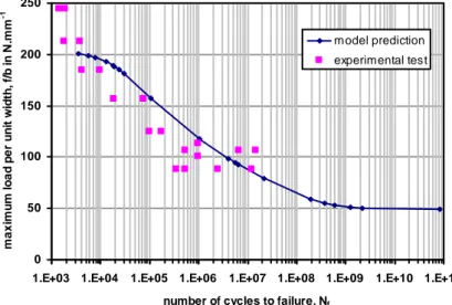
The model predictions are compared (see Figure 8) to experimental fatigue test result on single-lap-bonded joints (see Figure 1), provided in [2, 3], as well as the Paris law parameters and the Griffith flaw size required (see Table I). J is computed with Eqn. 21 and Eqn. 22. An encouraging correlation is then shown.

Gc Gth D n n1 n2 a0 450 J.m-2 85 J.m-2 3.64.10-20 m²/N cycle 5.61 3.20 9.34 85 µm Table I – Paris law parameters and Griffith flaw size employed

Figure 8 – Comparison of fatigue life predicted by the model (Eqn. 25 and Eqn. 26) with experimental test data extracted from [2, 3]

CONCLUSION

A 1D-beam approach for both stress analysis and fatigue life prediction of bonded joints is presented. Only the adhesive is supposed to fail. The 1D-beam model is developed in an extended Goland and Reissner framework [1] by considering unbalanced laminated or monolithic beams under thermal loading. The method employed [4] takes benefit of the flexibility of FE method, since it allows, thanks to a computer programme, both for the resolution of the entire set of equations and for the simple simulation of crack propagation in the adhesive layer through simple manipulations. It is underlined that one macro-element is enough to simulate a full bonded overlap. Simplified expressions of the J-integral parameters are expressed as a function of the load conditions and employed as a fracture criterion. This is then introduced through a modified Paris law for the crack propagation simulation. An encouraging correlation with published [2, 3] experimental results is shown. The thermal mismatch effect could be simply approximated by applying the equivalent thermal nodal forces; it remains to be assessed.

ACKNOWLEDGMENTS

0 50 100 150 200 250

1.E+03 1.E+04 1.E+05 1.E+06 1.E+07 1.E+08 1.E+09 1.E+10 1.E+11

number of cycles to failure, Nf

m a x im u m l o a d p e r u n it w id th , f/ b i n N .m m -1 model prediction experimental test

The authors gratefully acknowledge the SOGETI HIGH TECH engineers and managers – especially the “bolted joint method and research team” – involved in the development of JoSAT (Joint Stress Analysis Tool) internal research program.

REFERENCES

[1] Goland, M. and Reissner, E. (1944), J. Appl. Mech., vol. 11, pp. A17-27 [2] Curley, A.J., Hadavinia, H., Kinloch, A.J. and Taylor, A.C. (2000), Int. J. Fract., vol. 103, pp. 41-69.

[3] Hadavinia, H., Kinloch, A.J., Little M.S.G. and Taylor, A.C. (2003), Int. J. Adhesion Adhesives, vol. 23, pp. 463-471.

[4] Paroissien, E., Sartor, M., Huet, J. and Lachaud, F. (2007), AIAA J. Aircraft., vol. 44, n. 2, pp. 573-582.

[5] Fraisse, P. and Schmidt, F. (1993), Int. J. Fract., vol. 63, pp. 59-73. [6] Tong, L. (1996), Acta Mech., vol. 117, pp. 101-113.

[7] Tong, L. (1998), Int. J. Solids Structures, vol. 35, n. 20, pp. 2601-2616. [8] Högberg, J.L. (2004). Thesis for the degree of licentiate of engineering, Chalmers University of Technology, Göteborg, Sweden.

[9] SCILAB, v4.1.2, 23/10/2007, INRIA/ENPC [10] SAMCEF, v13.1-01, 25/06/2009, Samtech Group

[11] Dechwayukul, C., Rubin, C.A. and Hahn, G. T. (2003), AIAA J.., vol. 41, n. 11, pp. 2216-2228

APPENDIX A

This appendix details the resolution of the differential in Eqn. 8, which is identical for both adhesive stresses. The characteristic polynomial expression is:

                       4 1 3 2 4 1 2 2 3 k k k k dˆ k cˆ k bˆ 1 aˆ r R 0 dˆ R cˆ R bˆ R aˆ ) R ( P (27) To determine these roots, the Cardan’s method is employed. Then, Eqn 25 is modified as:

                      4 1 3 2 4 2 1 1 4 2 1 3 k k k k ) k 9 k 2 ( 27 k q ˆ k 3 k p ˆ 0 qˆ R p ˆ R (28) where: 3 k R R  1 (29) and the determinant is:

3 2 p ˆ 27 4 qˆ ˆ_{ }  (30) By defining:              3 3 2 ˆ qˆ vˆ 2 ˆ qˆ uˆ   (31) The roots of the reduced equation are written as:

               vˆ j uˆ j R vˆ j uˆ j R vˆ uˆ R 2 2 3 2 1 (32) Consequently, the roots of the characteristic equation (Eqn 25) are given by:

                             2 1 3 2 1 2 2 1 1 ) it s ( ) vˆ uˆ ( 2 3 i 3 k ) vˆ uˆ ( 2 1 R ) it s ( ) vˆ uˆ ( 2 3 i 3 k ) vˆ uˆ ( 2 1 R r 3 k vˆ uˆ R (33) Finally, the adhesive stresses have to be determined through Eqn. 29 where:

)) R Re( R ( 2 1 t ; ) R ) R (Re( 2 1 s ; 3 k vˆ uˆ r   1  ₂  ₂  ₂  ₂ (34)

APPENDIX B

The stiffness matrix of a beam element KB can be expressed in the base u, w, 

                                                             _                   i i i i i i i i i i 2 i i i 2 i i i i i i i i i i i i i i 2 i i i 2 i i i i i i 2 i i i 2 i i i 3 i i i 3 i i i 2 i i i 2 i i i 3 i i i 3 i i i i i i i i i i i i i i i i B D A 3 l 1 D A 3 l 1 A l 6 A l 6 l B l B D A 3 l 1 D A 3 l 1 A l 6 A l 6 l B l B A l 6 A l 6 A l 12 A l 12 0 0 A l 6 A l 6 A l 12 A l 12 0 0 l B l B 0 0 l A l A l B l B 0 0 l A l A K                 (35)