Volume 8, Issue 1 2012 Article 22
Biostatistics
Testing the assumptions for the analysis of
survival data arising from a prevalent cohort
study with follow-up
Vittorio Addona, Macalester College
Juli Atherton, Université du Québec à Montréal
David B. Wolfson, McGill University
Recommended Citation:
Addona, Vittorio; Atherton, Juli; and Wolfson, David B. (2012) "Testing the assumptions for the analysis of survival data arising from a prevalent cohort study with follow-up," The
survival data arising from a prevalent cohort
study with follow-up
Vittorio Addona, Juli Atherton, and David B. Wolfson
Abstract
In a prevalent cohort study with follow-up subjects identified as prevalent cases are followed until failure (defined suitably) or censoring. When the dates of the initiating events of these prevalent cases are ascertainable, each observed datum point consists of a backward recurrence time and a possibly censored forward recurrence time. Their sum is well known to be the left truncated lifetime. It is common to term these left truncated lifetimes "length biased" if the initiating event times of all the incident cases (including those not observed through the prevalent sampling scheme) follow a stationary Poisson process. Statistical inference is then said to be carried out under stationarity. Whether or not stationarity holds, a further assumption needed for estimation of the incident survivor function is the independence of the lifetimes and their accompanying truncation times. That is, it must be assumed that survival does not depend on the calendar date of the initiating event. We show how this assumption may be checked under stationarity, even though only the backward recurrence times and their associated (possibly censored) forward recurrence times are observed. We prove that independence of the lifetimes and truncation times is equivalent to equality in distribution of the backward and forward recurrence times, and exploit this equivalence as a means of testing the former hypothesis. A simulation study is conducted to investigate the power and Type 1 error rate of our proposed tests, which include a bootstrap procedure that takes into account the pairwise dependence between the forward and backward recurrence times, as well as the potential censoring of only one of the members of each pair. We illustrate our methods using data from the Canadian Study of Health and Aging. We also point out an equivalence of the problem presented here to a non-standard changepoint problem.
KEYWORDS: prevalent cohort study, left truncation, backward recurrence time, forward
recurrence time, censored mathced pairs
Author Notes: We thank two anonymous referees for their thoughtful comments and suggestions
which helped greatly improve our paper. The data reported in this article were collected as part of the Canadian Study of Health and Aging. The core study was funded by the Seniors' Independence Research Program, through the National Health Research and Development Program (NHRDP) of Health Canada Project 6606-3954-MC(S). Additional funding was provided by Pfizer Canada Incorporated through the Medical Research Council/Pharmaceutical Manufacturers Association of Canada Health Activity Program, NHRDP Project 6603-1417-302(R), Bayer Incorporated, and the British Columbia Health Research Foundation Projects 38 (93-2) and 34 (96-1). The study
1
Introduction
In a prevalent cohort study with follow-up subjects identified as prevalent cases are followed until failure (defined suitably) or censoring. For example, in the Canadian Study on Health and Aging (CSHA) [1] subjects with prevalent dementia were followed until death or censoring and the survival data collected provided the basis for estimation of survival from onset of dementia [2]. Prevalent cohort studies with follow-up are often carried out in preference to incident cohort studies which can entail prohibitive costs and lengthy follow-up of very large cohorts of initially disease-free subjects.
When the dates of the initiating events of the prevalent cases are ascertain-able, each observed datum vector consists of a backward recurrence time, a possibly censored forward recurrence time, and a censoring indicator. The sum of the back-ward and forback-ward recurrence times is well known to be the left truncated lifetime. It is common to term these left truncated lifetimes “length biased” if the initiating events of all cases (including those cases not observed in the prevalent cohort) fol-low a stationary Poisson process. Statistical inference is then said to be carried out under stationarity. For several formal approaches to the assessment of stationarity, see [3] and [4], whose methods are based on testing for the equality in distribution of the backward and forward recurrence times. Whether or not stationarity holds, a further assumption is almost always made. This is the assumption that the under-lying, incident, lifetimes are independent of their accompanying truncation times. See, for example, [5, 6, 7].
Arbitrarily left truncated survival data cannot be used to test for indepen-dence between failure times and truncation times without further special model assumptions, for example, about the initiation process. The problem is that only a biased subset of the lifetimes and truncation times is observed and quantification of this bias is impossible in a completely general nonparametric setting. We there-fore make the assumption of stationarity, which is equivalent to the assumption of a constant incidence rate for the Poisson initiation process. We place no restriction on the survivor function. In this setting, we show that the observed data consist-ing of the length biased truncation times (backward recurrence times and, possibly censored, forward recurrence times), may be used to test the assumption of inde-pendence. Our work complements that of [8], who discuss a nonparametric test for quasi-independence between lifetimes and truncation times based on Kendall’s tau, and that of [4], in that it provides another role for testing the equality of the backward and forward recurrence time distributions. We also provide an alternative bootstrap testing procedure.
The structure of the paper is as follows: In Section 2 we present notation, and in Section 3 we introduce the assumptions made in our work. In Section 4 we
state our main theorems, and in Section 5 we describe how these may be invoked to test for independence. We carry out a simulation study to assess the power and Type 1 error rate of our proposed tests in Section 6. Section 7 contains the results obtained from applying our methodology to data collected during the CSHA, in order to determine whether survival with dementia from onset changed over a pe-riod before 1991. In Section 8, we discuss the link of the current work to that of a non-standard changepoint problem, and also to that of testing if there has been “pre-recruitment censoring”, since another common assumption made in the literature is that no censoring can occur before recruitment into a prevalent cohort.
2
Notation and preliminaries
Let X1, . . . , Xm be independent and identically distributed (i.i.d.) positive random
variables representing lifetimes. If the survivor function of X1, . . . , Xm does not
change with calendar time, we represent the common survivor function as H(x), and the corresponding probability density function (p.d.f.) as h(x). Let τ1, τ2, . . . , τmbe
the corresponding calendar times of initiation, for convenience, termed onset, which are assumed to arise from a stationary Poisson process. Also, let τ∗be the calendar time of recruitment of prevalent cases into the study. Individual i is observed if Xi≥
τ∗− τi. Thus, the data is left-truncated, with left-truncation time Ti= τ∗− τi. Since
the initiation times arise from a stationary Poisson process, the Ti’s are uniform
random variables, with constant p.d.f. g(t).
Let Y1, . . . ,Ynbe the observed left-truncated lifetimes, with n ≤ m, recalling
that some individuals will go unobserved. That is, for observed lifetime Y , lifetime X, and truncation time T , P(Y > x) = P(X > x|X ≥ T ).
For an observed individual i, we write Yi = Yibwd+ Y f wd
i , where Yibwd is
the time from onset to recruitment, or the backward recurrence time (i.e. current lifetime), and Yif wdis the time from recruitment to failure, or the forward recurrence time(i.e. residual lifetime). We let the p.d.f. of Yibwdand Yif wd be, respectively, fbwd
and ff wd, and note that Yibwd and Y f wd
i are negatively correlated conditional on a
fixed value of Yi.
We denote the right-censoring time of subject i by Ci. We have that Ci=
Yibwd+Ci∗, where Ci∗, the residual censoring time, is the time from recruitment until the subject is censored. Hence, the observed data are (Yibwd,Yiobs, δi), i = 1, 2, . . . , n,
where Yiobs= min(Yif wd,Ci∗), and δi= 1[Yif wd ≤ Ci∗] is the usual censoring indicator
3
Independence between lifetimes and truncation
times
The main purpose of this paper is to propose a test of independence between the lifetimes, X , and the left-truncation times, T , under mild assumptions, by using the data (Yibwd,Yiobs, δi), i = 1, 2, . . . , n. As we have pointed out in the introduction, this
independence cannot be assessed for arbitrarily left-truncated survival data. Our main result, stated formally in Theorem 2, is that under stationarity and other mild assumptions, independence of X and T is equivalent to the equality of Yibwd and Yif wd in distribution. Let
S(x;t) = P(X > x | T = t) (1)
represent the survivor function for a subject with onset at calendar time (τ∗− t). Lemma 1 below allows us to transfer statements about independence between X and T to statements about S(x;t).
Lemma 1. Let X and T represent a lifetime, and left-truncation time, respectively. Then, X and T are independent if and only if S(x;t) = H(x); that is, the survivor function is independent of the date of onset (equivalently, the truncation time). Proof: X ⊥ T ⇔ S(x;t) = P(X > x|T = t) = P(X > x) = H(x) ∀ x,t > 0.
Before formally stating our main theorems, we introduce four assumptions. These assumptions will be seen to be reasonable in many applications.
Assumption 1 (A1): P(Ci> Ti) = 1 for all i.
Assumption 2 (A2): For all i, the residual censoring times Ci∗are independent of both Yif wd and Yibwd.
Assumption 3 (A3): The incidence process is stationary.
Assumption 4 (A4): Let X (t) and X (t0) be lifetimes from the survivor func-tions S(x;t) and S(x;t0), respectively, where 0 ≤ t ≤ t0. Letting ≤st and ≥st represent the stochastic orderings, then either, X (t) ≤st X(t0) or X (t) ≥st X(t0), ∀ 0 ≤ t ≤ t0.
3.1
Discussion of Assumptions
A1 ensures that there is no “pre-recruitment censoring”, a standard assump-tion made in the literature. See, however, further discussion on this issue in Section 8.
A2 specifies that the forward recurrence times are randomly right censored by their corresponding residual censoring times. It also specifies that residual censoring is not influenced by the date of initiation for those that are part of the prevalent cohort.
A3 ensures (in the presence of the other assumptions) that our methods are ap-plicable to diseases such as multiple sclerosis and Alzheimer’s disease which have roughly constant incidence rates over short time intervals - of length, say, 20 years. Our methods would not be applicable to diseases whose inci-dence rates change rapidly.
A4 allows survival only to possibly improve or worsen as a function of initi-ation date. This might be the case, for example, following the introduction of an effective treatment prior to recruitment. Fluctuations in survival - rare, in any case - are not permitted.
4
Main theorems
Theorem 1 is concerned with the alternative hypothesis. It gives reasonable alter-natives in terms of the survivor functions, S(x;t) and S(x;t0), t < t0(see assumption A4), which is equivalent to the stochastic ordering of the forward and backward re-currence times. Theorem 2 gives two statements, (a) and (b), which are equivalent to the null hypothesis, (c), of equality in distribution of the forward and backward recurrence times. The hypothesis (c) is primarily of interest because it provides a simple mechanism for testing the hypotheses (a) and (b). The stochastic ordering of the forward and backward recurrence times is a natural alternative to the null hypothesis (c) of Theorem 2. Together, Theorems 1 and 2 prepare the way for a simple test of independence between the truncation time and the failure time. Theorem 1. Under assumptions A1-A4 the following statements are true: (a) S(x;t) < S(x;t0) for t < t0and∀x > 0 ⇔ Sf wd(x) < Sbwd(x) ∀x > 0. (b) S(x;t) > S(x;t0) for t < t0and∀x > 0 ⇔ Sf wd(x) > Sbwd(x) ∀x > 0.
Proof. We prove (a). Part (b) is shown in a similar fashion. Letting D be a constant, it is shown in Section 9.1, in the Appendix, that
Sf wd(x) = D Z ∞ 0 S(u + x; u)du Sbwd(x) = D Z ∞ 0 S(u + x; u + x)du
(⇒) If S(x;t) < S(x;t0) ∀ t < t0 and x > 0, then ∀ u > 0, x > 0, S(u + x; u + x) > S(u + x; u). Hence Sf wd(x) < Sbwd(x).
(⇐)
Sf wd(x) < Sbwd(x) (2)
is equivalent toR∞
0 S(u + x; u)du <
R∞
0 S(u + x; u + x)du and under A1-A4 the three
options for S(x;t) are that either,
S(x;t) is stochastically increasing in calendar time, or S(x;t) is constant (= H(x)) in calendar time, or S(x;t) is stochastically decreasing in calendar time.
Clearly (2) is satisfied only if S(x;t) is stochastically increasing.
Theorem 2. Under assumptions A1-A4, (a), (b), and (c) below are equivalent: (a) Xiand Tiare independent∀ i.
(b) S(x;t) = H(x) ∀ t ≥ 0 and ∀ x ≥ 0. (c) ff wd(x) = fbwd(x) ∀ x ≥ 0.
Proof: See Section 9.2, in the Appendix.
5
Testing
The development thus far has been with the goal of testing for independence be-tween lifetimes and truncation times. In view of Theorems 1 and 2, testing for independence reduces to testing,
H0: Yf wd =DYbwd (3)
vs. Ha: Yf wd >stYbwd (or Yf wd <stYbwd),
under the assumptions A1-A4.
Since the components of each pair (Yibwd, Yif wd) are conditionally depen-dent given the lifetime, a distribution-free matched pairs test is suggested. But, the allowance for the possible censoring of Yif wd prevents a straight application of the Wilcoxon signed rank test. Wei [9] used the same scoring function as [10] and
[11] to construct an asymptotically distribution-free test for the null hypothesis of bivariate symmetry when the data are paired observations where both components may be right-censored. Wei’s test is a modified two-sample Wilcoxon rank sum test which makes use of both within pair, and between pair, comparisons [9]. Al-ternative hypotheses considered in [9] include the class of alAl-ternatives induced by stochastic ordering. We note that, although bivariate symmetry of a joint distribu-tion funcdistribu-tion implies equality of the marginal distribudistribu-tions, the converse is not true in general. When the pairs correspond to backward and forward recurrence times, however, the two hypotheses are indeed equivalent [3], permitting the application of Wei’s test to the problem of interest in the current paper. That is, in conjunction with the characterizations provided by Theorems 1 and 2, one option to test inde-pendence between lifetimes and truncation times, via the hypotheses in (3), would be to carry out Wei’s test for censored, paired data [9].
Specifically, we proceed by defining a scoring function which is a natural generalization of the Mann-Whitney scoring function to the right-censoring case, in that it assigns non-zero values only to observed pairs where one member is known to be larger than the other (there may be ambiguity about the ordering of the two random variables in the presence of censoring). The scoring function, Ψ, is defined for each of the n2comparisons as follows:
Ψ(Yibwd,Yjobs, δj) = 1[Yibwd > Yjobs, δj= 1] − 1[Yibwd < Yjobs] (4)
Let Wn= n12∑ni=1∑nj=1Ψ(Yibwd,Yjobs, δj). Under H0, Wei shows that, as n → ∞,
√
nWnconverges to a Normal random variable with mean, 0, and variance, σ2, and proposes an estimator, ˆσ2, of σ2 [9]. An asymptotically nonparametric test com-pares the observed absolute value of
√ nWn
ˆ
σ with the upper α-quantile of the standard
Normal distribution. Cheng [12] points out that the test in [9] is conservative. He provides an alternative estimator of σ2 to address this drawback, but it is only ap-propriate if the censoring distributions of the members of each pair are identical, which is not the case in our setting. One might thus worry that Wei’s test has insuf-ficient power to detect dependence between the lifetimes and the truncation times.
An alternative approach to the two sample problem presented in (3) is to use a logrank test. Another possibility is to compare the distributions of the backward and forward recurrence times through a Kolmogorov-Smirnov type statistic, based on the two estimated survival functions. A straight application of either of these op-tions is not possible, however, due to the within pair correlation that exists between Yibwd and Yif wd. We address this issue by proceeding with a bootstrap technique (described below) to obtain the null distribution of the logrank test statistic.
Bootstrap Procedure:
1. Sample from the triplets, (Yibwd,Yiobs, δi), with replacement to obtain a new
set of n triplets.
2. With the set of resampled triplets, find the nonparametric maximum likeli-hood estimate of the length-biased distribution [13].
3. From the estimated length-biased distribution, generate n length-biased sur-vival times. These are “pure” failure times, i.e. they are not subject to cen-soring.
4. Generate pure backward and forward recurrence times by multiplying each length-biased failure time from 3. by a uniform(0,1) random variable. This ensures that the backward and forward recurrence times are generated under H0.
5. Using the n resampled triples from 1. find the Kaplan-Meier estimate of the residual censoring distribution by reversing the roles of the censored, and exact, forward recurrence times. Generate n residual censoring times from this Kaplan-Meier estimate.
6. Randomly match the n residual censoring times from 5. with the n pure for-ward recurrence times from 4. and, in each case, record the usual censoring indicator. Using the corresponding pure backward recurrence times from 4., form the n triples generated under H0.
7. From the triplets formed in 6. compute a logrank statistic based on the two groups: backward recurrence time and (possibly censored) forward recur-rence time.
8. Repeat steps 1. to 7. many times, recording the logrank statistics, to obtain a bootstrap null distribution of this test statistic.
9. Obtain a bootstrap p-value by computing the observed logrank statistic from the original data, (Yibwd,Yiobs, δi), and finding the proportion of bootstrapped
statistics as large or larger than the observed statistic.
Our bootstrap procedure maintains the negative correlation between the backward and forward recurrence times, conditional on the value of their sum. Moreover, it preserves the censoring structure of no possibility of censoring of the backward recurrence times, and possible right-censoring of the forward recurrence times.
6
A power study
We carried out a power study of Wei’s test and our bootstrap procedure for detect-ing whether survival depends on the date of onset. We generated onsets assumdetect-ing
stationarity, and a survival time for each onset, in the following fashion: if the onset date was within ˜xof τ∗(calendar time of recruitment), for some ˜x, then the lifetime was generated from the p.d.f. h1; otherwise, the lifetime was generated from the
p.d.f. h2, where h1and h2satisfy A4. Thus, we allowed survival to change at a
sin-gle point in time, (τ∗− ˜x). The observed sample consisted of those lifetimes which extended beyond τ∗.
6.1
Details of the simulations for Wei’s test
We investigated the power and size of Wei’s test using sample sizes of n = 500 and n= 1000, and two h2’s: Weibull(γ=2, β2=10) and Lognormal(µ2=1.75, σ =0.4),
where the Weibull and Lognormal are parameterized as follows:
Weibull(γ, β ) : γ β xγ −1e−xγβ 1[x > 0] and, Lognormal(µ, σ ) : e −(logx−µ)2 2σ 2 √ 2πσ x 1[x > 0] .
In determining how survival changed at (τ∗− ˜x), we investigated varying degrees of improving and worsening survival. For both the Weibull and the Log-normal cases, six choices of h1 were used: Weibull(γ=2, β1) and Lognormal(µ1,
σ =0.4), where β1= 13.25, 15, 17, 7.25, 6, 5, and µ1 = 1.89, 1.95, 2.01, 1.59, 1.50,
1.39. The parameter values β1 = 13.25, 15, 17, and µ1 = 1.89, 1.95, 2.01,
repre-sent improvements in survival, and correspond, respectively, to approximately 15%, 22.5%, and 30% increases in mean survival after (τ∗− ˜x). The parameter values β1
= 7.25, 6, 5, and µ1 = 1.59, 1.50, 1.39, represent declines in mean survival after
(τ∗− ˜x) of approximately 15%, 22.5%, and 30%, respectively. We also investigated the size of Wei’s test by setting h1= h2.
We chose the residual censoring time distribution to be Exponential, and such that approximately 25% or 35% of the forward recurrence times were cen-sored. The value of ˜x determines how far from recruitment the change in survival occurred. If ˜x is small it will be difficult to detect this change since few subjects will be observed who experienced h1. Similarly, if ˜x is large it will be difficult to
detect the change in survival since few individuals who experienced h2will survive
long enough to be observed. The mean of our choices for h2 were 2.80 (Weibull)
and 6.23 (Lognormal). We thus chose ˜x= 2 or 3, and ˜x= 5 or 7, for the Weibull and Lognormal cases, respectively.
The two sample sizes, two censoring percentages, seven choices of h1, and
two values of ˜xled to fifty-six distinct simulation scenarios for both the Weibull and Lognormal distribution. For each, we recorded the number of two-sided rejections, at the 5% level, in 200 replicates.
6.2
Details of the simulations for bootstrap procedure
We implemented a more limited power study for the bootstrap procedure presented in Section 5, as it is considerably more time consuming to carry out. Of the scenar-ios described in Section 6.1, we focused on the Weibull distribution, with ˜x= 2 and n= 500. Fourteen simulation scenarios remained, and we recorded the number of rejections, at the 5% level, in 50 replicates.
6.3
Results of the simulations
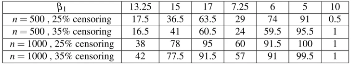
The rejection percentages are presented in Tables 1-4 for Wei’s test, and in Table 5 for our bootstrap procedure. The last column in each table is for the case of no change in survival, that is, the Type 1 error percentages.
Table 1 illustrates that, when n = 1000, Wei’s test had good power except for the smallest changes in survival (i.e. β1=13.25, β1=7.25). When n = 500, however,
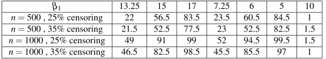
only the largest decrease in survival was almost always detected. From Table 2, we see that when n = 500, only the biggest changes in survival were adequately detected, but increasing the sample size to n = 1000 substantially improved power. Tables 3 and 4 display similar results. In Table 3, we see adequate power except for the smallest changes in survival with n = 500. Table 4 shows that Wei’s test had poor power against the smallest changes in survival (particularly when n = 500), and generally inadequate power when n = 500. Finally, the size of Wei’s test was considerably lower than the nominal 5%. This no doubt led to a loss in power as is demonstrated by the superior power of our bootstrap logrank test which, based on limited simulations, has a Type 1 error rate slightly larger than 5% (see Table 5).
β1 13.25 15 17 7.25 6 5 10
n= 500 , 25% censoring 17.5 36.5 63.5 29 74 91 0.5 n= 500 , 35% censoring 16.5 41 60.5 24 59.5 95.5 1 n= 1000 , 25% censoring 38 78 95 60 91.5 100 1 n= 1000 , 35% censoring 42 77.5 91.5 57 91 99.5 1
Table 1: Percentage of rejections for Weibull(γ=2, β2=10) with ˜x= 2 using Wei’s
β1 13.25 15 17 7.25 6 5 10
n= 500 , 25% censoring 22 56.5 83.5 23.5 60.5 84.5 1 n= 500 , 35% censoring 21.5 52.5 77.5 23 52.5 82.5 1.5 n= 1000 , 25% censoring 49 91 99 52 94.5 99.5 1.5 n= 1000 , 35% censoring 46.5 82.5 98.5 45.5 85.5 97 1
Table 2: Percentage of rejections for Weibull(γ=2, β2=10) with ˜x= 3 using Wei’s
test on 200 generated data sets.
µ1 1.89 1.95 2.01 1.59 1.50 1.39 1.75
n= 500 , 25% censoring 30.5 78 92 34.5 75.5 99 2 n= 500 , 35% censoring 32.5 67.5 91 32.5 74.5 92 1 n= 1000 , 25% censoring 65.5 96 100 72 99 100 2 n= 1000 , 35% censoring 67 94.5 100 66 96 99.5 1
Table 3: Percentage of rejections for Lognormal(µ2=1.75, σ =0.4) with ˜x= 5 using
Wei’s test on 200 generated data sets.
µ1 1.89 1.95 2.01 1.59 1.50 1.39 1.75
n= 500 , 25% censoring 20 43.5 83.5 13 37.5 58 1 n= 500 , 35% censoring 20.5 50.5 75.5 13 33.5 50 1.5 n= 1000 , 25% censoring 45.5 85.5 99.5 38 69 90 2
n= 1000 , 35% censoring 43 82.5 99.5 33 59.5 83 1
Table 4: Percentage of rejections for Lognormal(µ2=1.75, σ =0.4) with ˜x= 7 using
Wei’s test on 200 generated data sets.
β1 13.25 15 17 7.25 6 5 10
n= 500 , 25% censoring 56 90 100 70 98 100 4 n= 500 , 35% censoring 60 86 98 66 94 100 10
Table 5: Percentage of rejections for Weibull(γ=2, β2=10) with ˜x= 2 using
boot-strap logrank procedure on 50 generated data sets.
7
The Canadian Study of Health and Aging (CSHA)
We briefly describe the CSHA and show how our approach may be used to test whether the assumption of independence between onset date and survival time, prior to 1991, was reasonable. This assumption was crucial in the analysis
car-ried out by [2] and by [14], with the purpose of estimating survival with dementia, from onset. Furthermore, the independence assumption is necessary in a general nonparametric setting if one is to avoid model non-identifiability.
In 1991, a cohort consisting of 821 prevalent subjects with possible demen-tia, probable demendemen-tia, or vascular dementia was identified (termed CSHA1). Their onset dates were determined from their caregivers, and the cohort was followed un-til 1996, termed CSHA2 (see [2] and [14]). The dates of death or censoring, along with the dates of onset for all cohort members were used to estimate, nonparamet-rically, survival from onset, of subjects with dementia. In [2], a robust product limit estimator was used without the assumption of a stationary onset process, but with the unverifiable assumption of independence between onset date and length of sur-vival in the general left truncation setting. In [14], stationarity was assumed along with independence between onset date and length of survival. In this paper, we assume that the incidence rate of dementia remained roughly constant, say, twenty years prior to 1991, and test the assumption of independence between onset date and survival.
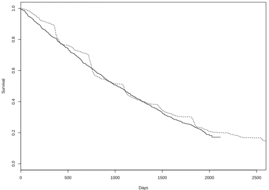
Using data obtained on the 821 subjects identified in CSHA1, that is, the approximate dates of onset of dementia and the dates of death or censoring, we present in Figure 1 the estimated backward and forward recurrence time distribu-tions. Since the backward recurrence times are not censored, the non-parametric maximum likelihood estimator (NPMLE) of the survivor function is the empirical survivor function, whereas the NPMLE of the forward recurrence time survivor function is a Kaplan-Meier estimator. The apparent periodicity in the backward recurrence time empirical survivor function is due to the tendency of caregivers to remember onset dates only to the nearest year.
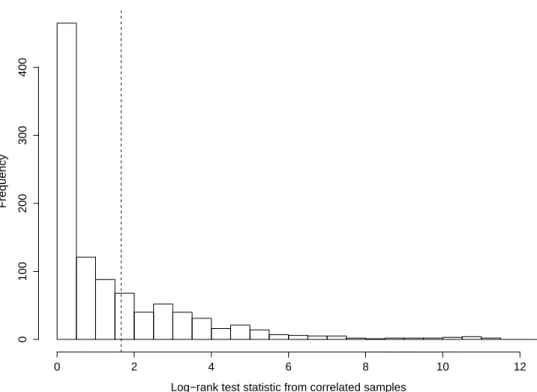
Employing our bootstrap procedure, with 1000 bootstrap replicates, we ob-tained the null distribution of the logrank test statistic from the dependent samples shown in Figure 2. The observed value of the logrank test statistic was 1.66, and it is also displayed in Figure 2 with a dashed vertical line. This yielded a bootstrap p-value of 0.295, consistent with the null hypothesis in (3), or equivalently, with independence between date of onset and survival.
The results of our bootstrap procedure are consistent with those obtained by carrying out Wei’s [9] test, which yielded a test statistic of 0.98 (to be compared with a standard Normal) and a two-sided p-value of 0.33. Thus, our data are con-sistent with the hypothesis of non-changing survival for dementia patients in the roughly 20 years prior to 1991.
0 500 1000 1500 2000 2500 0.0 0.2 0.4 0.6 0.8 1.0 Days Sur viv al
Figure 1: Estimated backward (dashed) and forward (solid) survival curves from the CSHA data.
8
Concluding remarks
A universal assumption made in the analysis of survival data from a prevalent cohort study with follow-up is that censoring can only occur after subjects are recruited into the study. Assumption A1 is reasonable since only subjects under follow-up can be lost to follow-up. Nevertheless, it is possible for a subject to leave the pop-ulation after onset but before recruitment, for example, due to migration or death from a competing risk. Interestingly, in these situations, the variable, C, which after recruitment is a censoring variable, becomes a (random) truncating variable before the recruitment date; those subjects who migrate after onset but before re-cruitment cannot be part of the prevalent cohort. Should such an additional layer of left-truncation occur, an analysis that is based on the stationarity assumption will not be valid. Therefore, one may wish to test whether there is truncation induced by C prior to recruitment. It is possible to show that, assuming stationarity and inde-pendence between X and T , the hypotheses in (3) may be used to test if P(Ci> Ti)
Log−rank test statistic from correlated samples Frequency 0 2 4 6 8 10 12 0 100 200 300 400
Figure 2: Null distribution using the bootstrap procedure described in Section 5, with observed test statistic shown as a dashed vertical line.
to the following conclusion: Consider the three assumptions: (i) stationarity, (ii) independence between X and T , and (iii) P(Ci> Ti) = 1. Fixing any two of these, it
is possible to test the third, using the hypotheses in (3), and the observable data. Suppose that the change in the distribution of survival times could occur only at a single point in time, so that subjects would experience different survival depending on whether they had onset before, or after, the calendar time of this change. In this case, Lemma 1 shows that the problem of testing for independence between X and T may be viewed as a changepoint problem with a twist. We wish to know whether a change has occurred in the survival time distribution before recruitment, where the changepoint is unknown. The unusual feature is that, unlike a classical changepoint problem, inference must be drawn from an incomplete set of (possibly censored) survival times – the incompleteness being induced by the left-truncation of X by T .
9
Appendix
9.1
Proof of Theorem 1
First, we find expressions which are proportional to the p.d.f. of Yibwd and Yif wd, respectively, in Lemma 2 below.
Lemma 2. Under assumptions A1-A4 and ∀ x ≥ 0, we have
1. fbwd(x) ∝ R∞
x f(x0; x)dx0
2. ff wd(x) ∝ R∞
x f(x0; x0− x)dx0,
where we define f(x;t) = f (x|T = t), the lifetime density given a left-truncation time, T = t, i.e. onset at calendar time (τ∗− t).
Proof. Let the random variables X , T , and Y represent a lifetime, a left-truncation time, and a left-truncated lifetime, respectively. The observed failure time p.d.f. is given by, fY(x) = Z x 0 fX,T(x,t|X ≥ T )dt = Z x 0 fX,T(x,t) P(X ≥ T )dt = Rx 0 f(x;t)g(t)dt P(X ≥ T )
Also, the backwards recurrence time p.d.f., conditional on the observed lifetime Y = x0, is given by, fbwd(x|Y = x0) = g(x|Y = x0) = fX,T(x0, x|X ≥ T ) fX(x0|X ≥ T ) = 1[xR0x0≥ x] f (x0; x)g(x) 0 f(x0;t)g(t)dt .
The backwards recurrence time p.d.f. is, fbwd(x) = Z ∞ x " f(x0; x)g(x) Rx0 0 f(x0;t)g(t)dt #"Rx 0 0 f(x0;t)g(t)dt P(X ≥ T ) # dx0 = R∞ x f(x0; x)g(x)dx0 P(X ≥ T ) .
Thus under stationarity we can write, fbwd(x) ∝
Z ∞
x
f(x0; x)dx0.
Since, ff wd(x|Y = x0) = fbwd(x0− x|Y = x0), we easily obtain the forward
recur-rence time p.d.f.:
ff wd(x) =
R∞
x f(x0; x0− x)g(x0− x)dx0
P(X ≥ T ) and under stationarity,
ff wd(x) ∝
Z ∞
x
f(x0; x0− x)dx0.
The proof of Theorem 1 is given in the text. Lemma 3 is required for that proof. Lemma 3. Under the usual conditions sufficient for the validity of Fubini’s Theo-rem we have, Sf wd(x) = D Z ∞ 0 S(u + x; u)du Sbwd(x) = D Z ∞ 0 S(u + x; u + x)du
Proof. Under stationarity g(x) = g(x0− x) = C, a constant. Letting D = P(X ≥T )C
Sf wd(x) = D Z ∞ x Z ∞ x∗ f(x0; x0− x∗)dx0dx∗ Sbwd(x) = D Z ∞ x Z ∞ x∗ f(x0; x∗)dx0dx∗ Sf wd(x) = D Z ∞ x Z ∞ x∗ f(x0; x0− x∗)dx0dx∗ = D Z ∞ x Z ∞ 0 f(x0+ x∗; x0)dx0dx∗
Using Fubini’s Theorem,
Sf wd(x) = D Z ∞ 0 Z ∞ x f(x0+ x∗; x0)dx∗dx0 = D Z ∞ 0 Z ∞ x0+x f(x∗; x0)dx∗dx0 = D Z ∞ 0 S(x0+ x; x0)dx0 = D Z ∞ 0 S(u + x; u)du Sbwd(x) = D Z ∞ x Z ∞ x∗ f(x0; x∗)dx0dx∗ = D Z ∞ x S(x∗; x∗)dx∗ = D Z ∞ 0 S(x∗+ x; x∗+ x)dx∗ = D Z ∞ 0 S(u + x; u + x)du
9.2
Proof of Theorem 2
(a)⇔ (b): See Lemma 1.
(b)⇒ (c): This follows immediately from Theorem 1 of [15]. It remains to establish that (c) ⇒ (b):
Proof. ff wd(x) = fbwd(x) ∀ x ≥ 0 implies that Sf wd(x) = Sbwd(x) ∀ x ≥ 0. But then
proceeding in a similar fashion as the proof of Theorem 1, it follows that S(x;t) = S(x;t0) ∀ t ≥ t0and x ≥ 0, which implies that part (b) of Theorem 2 holds.
References
1. Canadian Study of Health and Aging Working Group. The incidence of demen-tia in Canada. Neurology 2000;55:66-73.
2. Wolfson C, Wolfson DB, Asgharian M, M’Lan CE, Østbye T, Rockwood K, Hogan DB. A reevaluation of the duration of survival after the onset of dementia. New England Journal of Medicine 2001;344(15):1111-1116. 3. Addona V, Wolfson DB. A formal test for the stationarity of the incidence rate
using data from a prevalent cohort study with follow-up. Lifetime Data Analysis2006;12:267-284.
4. Mandel M, Betensky, RA. Testing Goodness of Fit of a Uniform Truncation Model. Biometrics 2007;63:405-412.
5. Gross ST, Lai TL. Nonparametric estimation and regression analysis with left-truncated data and right censored data. Journal of the American Statistical Association1996;435:1166-1180.
6. Turnbull B. The empirical distribution function with arbitrarily grouped, cen-sored and truncated data. Journal of the Royal Statistical Society, Series B 1976;38(3):290-295.
7. Wang M-C. Nonparametric estimation from cross-sectional survival data. Jour-nal of the American Statistical Association1991;86(413):130-143.
8. Martin EC, Betensky RA. Testing quasi-independence of failure and truncation times via conditional Kendall’s tau. Journal of the American Statistical Association2005;100(470):484-492.
9. Wei LJ. A generalized Gehan and Gilbert test for paired observations that are subject to arbitrary right censorship. Journal of the American Statistical Association1980;75(371):634-637.
10. Gehan EA. A generalized Wilcoxon test for comparing arbitrarily singly-censored samples. Biometrika 1965;52(3):650-653.
11. Gilbert JP. Random censorship. PhD Thesis. University of Chicago: Depart-ment of Statistics1962.
12. Cheng, KF. Asymptotically nonparametric tests with censored paired data. Communications in Statistics−Theory and Methods 1984;13(12):1453-1470.
13. Vardi, Y. Multiplicative censoring, renewal processes, deconvolution and de-creasing density: Nonparametric estimation. Biometrika 1989;76(4):751-761.
14. Asgharian M, M’Lan CE, Wolfson DB. Length-biased sampling with right cen-soring: an unconditional approach. Journal of the American Statistical As-sociation2002;457:201-209.
15. Asgharian M, Wolfson DB, Zhang Z. Checking stationarity of the inci-dence rate using prevalent cohort survival data. Statistics in Medicine 2005;25(10):1751-1767.