Fouille de données basée algorithmes bio-inspirés

(1)

Ministry of Higher Education and Scientific

Research

University of Ferhat Abbas Setif

-1-Thesis

Presented to the Faculty of Sciences Computer Science department

to obtain the title of

PhD of Science

Specialty : COMPUTER

SCIENCE

Defended by

Djaafar ZOUACHE

Bio-inspired Algorithms for Data

Mining

Defended on April 11, 2016

Jury:

President : Abdellah KHABABA Prof. University of Ferhat Abbas Setif -1 Advisor : Abdelouahab MOUSSAOUI Prof. University of Ferhat Abbas Setif -1

Examinators : Salim CHIKHI Prof. University of Constantine 2

Mohamed Tarek KHADIR Prof. University of Annaba

Mustapha BOURAHLA MCA. University of M’sila

(2)

République Algérienne Démocratique et Populaire

Ministère de l’Enseignement Supérieur et de la

Recherche Scientifique

Université Ferhat Abbas de Sétif

-1-Thèse

Présentée à la Faculté des Sciences Département d’Informatique En vue de l’obtention du diplôme de

Doctorat en Sciences

Option : INFORMATIQUE

Par

Djaafar ZOUACHE

Thème

Fouille de données basée

algorithmes bio-inspirés

Soutenu le: / /2015 devant le jury composé de :

Président : Abdellah KHABABA Prof. Université de Sétif 1

Rapporteur : Abdelouahab MOUSSAOUI Prof. Université de Sétif 1

Examinateurs : Salim CHIKHI Prof. Université de Constantine 2

Mohamed Tarek KHADIR Prof. Université d’Annaba

Mustapha BOURAHLA MCA. Université de M’sila

(3)

I would like to express my deep gratitude to my supervisors, Pr. Abdelouahab MOUSSAOUI, for his invaluable advice, time and support throughout this re-search work. This thesis would not have been possible without his encourage-ment, motivation, inspiration, and guidance.

I would like to thank Pr. Abdallah KHABABA, Pr. Salim CHIKHI, Pr. Mo-hamed Tarek KHADIR, Dr. Mustapha BOURAHLA, and Dr. MoMo-hamed SAIDI for accepting to be members of the examination committee for this thesis and for tak-ing time to read and review it. Their suggestions will be taken into account and will surely significantly improve the final version.

Last but not least, I wish to thank my family for their love, encouragement and support.

(4)

List of Tables

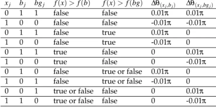
3.1 Lookup table of the rotation angle (x: binary individual, b: best local

solution, bg: best global solution, f (.): fitness function ) . . . 33

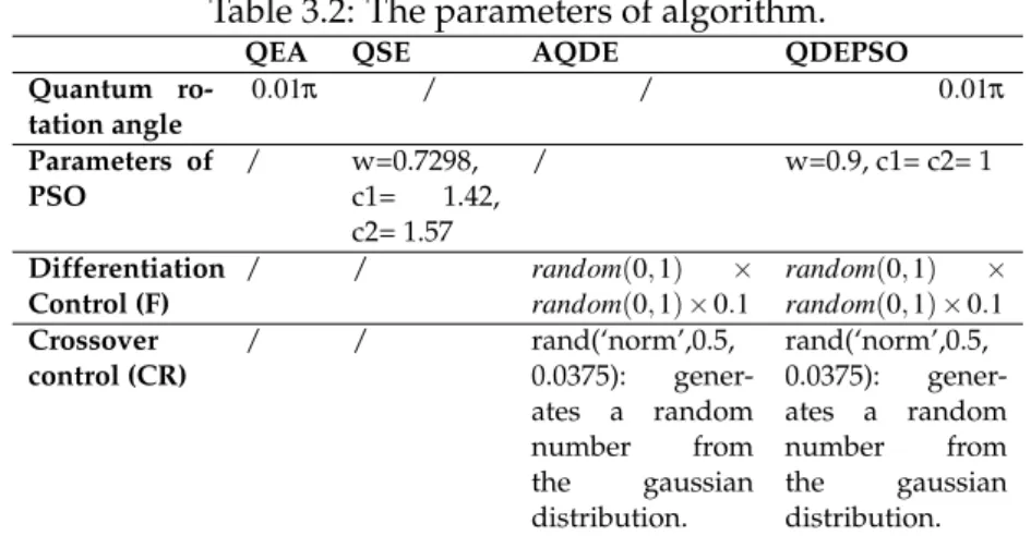
3.2 The parameters of algorithm. . . 34

3.3 Experimental results of the 0-1 knapsack problem (experiment 1). . . 35

3.4 The results of QDEPSO algorithm with selection of DE, without se-lection of DE, and with sese-lection of GA on the 0-1 knapsack problem (experiment 1).. . . 38

3.5 The QDEPSO algorithm without crossover of DE, with DE crossover, with single point crossover of GA and with two point crossover of GA.. . . 39

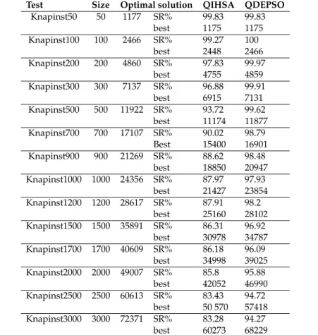
3.6 The Results of QDEPSO and QIHSA on the 0-1 knapsack (experi-ment 2). . . 40

4.1 Parameters of the algorithms . . . 56

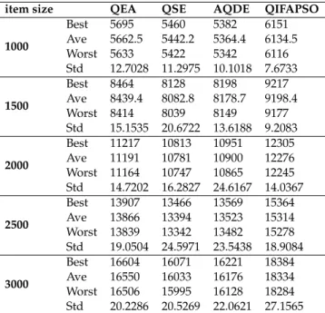
4.2 Comparison of QIFAPSO with QEA, QSE and AQDE on the 0-1 knapsack problem. . . 56

4.3 Performances of QIFAPSO algorithm without repairing, without PSO and with repairing and PSO (mknapcb1, mknapcb4). . . 60

4.4 Comparison between QIFAPSO algorithm and MBPSO, BPSOT-VAC and CBPSOTBPSOT-VAC algorithms on low-dimensional knapsack instances (Sento, Weing). . . 61

4.5 Comparison between QIFAPSO algorithm and MBPSO, BPSOT-VAC and CBPSOTBPSOT-VAC algorithms on low-dimensional knapsack instances (Weish). . . 62

4.6 Comparison between QIFAPSO, BPSOTVAC and CBPSOTVAC al-gorithms on high-dimensional knapsack instances (mknapcb3-5-500). 63 4.7 Comparison between QIFAPSO algorithm and SACRO-BPSO-TVAC, SACRO-CBPSO-TVAC and BHTPSO. . . 64

4.8 Comparison between QIFAPSO algorithm and BAPSA, BPSAL and BPSOL. . . 65

5.1 Data description. . . 74

5.2 Performance comparison on discrete datasets. . . 75

5.3 QIFAPSO-FS exploration process on vote. . . 77

(9)

5.5 QIFAPSO-FS exploration process on exactly2. . . 77

5.6 QIFAPSO-FS exploration process on DNA. . . 77

5.7 QIFAPSO-FS exploration process on dermatology. . . 78

5.8 Reduct sizes found by feature selection algorithms. . . 80

5.9 Minimal number of iterations to find the best subset of features by metaheuristic algorithms. . . 80

(10)

List of Figures

2.1 Feature selection process [Dash 1997]. . . 17

2.2 A filter feature selection algorithm [Xue 2014]. . . 17

2.3 A wrapper feature selection algorithm [Xue 2014]. . . 18

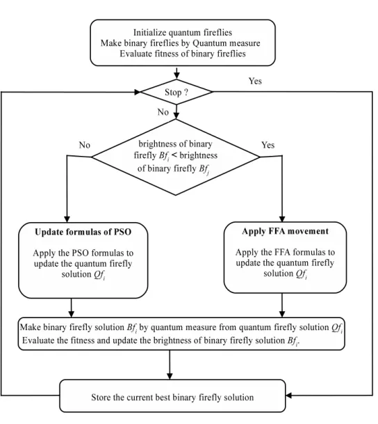
3.1 The global architecture of the QDEPSO algorithm. . . 28

3.2 Average profits (250 items). . . 35

3.5 Best profits (250 items) . . . 36

3.8 Average profits of QDEPSO algorithm with selection of DE, without selection of DE and with selection of GA (100 items). . . 37

3.9 Average profits of QDEPSO algorithm with selection of DE, without selection of DE and with selection of GA (2000 items). . . 38

3.10 Success rate versus items’ size. . . 39

4.1 Global architecture of QIFAPSO algorithm . . . 47

4.2 Q-bit representation by the unity circle . . . 48

4.3 Discrete distance between two binary fireflies’ solutions. . . 51

4.4 Average profits (2000 items) . . . 57

4.6 Average profits (3000 items) . . . 57

4.8 Performances of QIFAPSO algorithm without repairing, without PSO and with repairing and PSO on mknapcb 1-5.100-05 . . . 59

4.9 Performances of QIFAPSO algorithm without repairing, without PSO and with repairing and PSO on mknapcb 4-10.100-05 . . . 59

4.10 Comparing MBPSO, BPSOTVAC, CBPSOTVAC and QIFAPSO wrt anova test for the multidimensional instances sento, and weing. . . . 63

4.11 Comparing BPSOTVAC, CBPSOTVAC and QIFAPSO wrt anova test for the multidimensional instances mknapcb3-5-500. . . 64

4.12 Comparing QIFAPSO, BPSOL, BAPSAL and BAPSA with Friedman test for multidimensional knapsack instances of mknapcb1 and mk-napcb4. . . 64

(11)

5.1 Reduction rate given by QIFAPSO-FS for all datasets. . . 76 5.2 Accuracy classification given by tree decision for raw data and best

subset find by QIFAPSO-FS. . . 76 5.3 Accuracy classifications given by KNN algorithm for raw data and

best subset find by QIFAPSO-FS. . . 76 5.4 Evolution exploration process of the global best on dataset vote by

QIFAPSO-FS algorithm. . . 78 5.5 Evolution exploration process of the global best on dataset

mush-room by QIFAPSO-FS algorithm. . . 78 5.6 Evolution exploration process of the global best on dataset exactly2

by QIFAPSO-FS algorithm.. . . 79 5.7 Evolution exploration process of the global best on dataset DNA by

QIFAPSO-FS algorithm. . . 79 5.8 Evolution exploration process of the global best on dataset

(12)

List of Algorithms

2.1 Particle Swarm Optimization . . . 12

2.2 Differential Evolution Algorithm . . . 14

2.3 Firefly Algorithm . . . 16

3.1 Observe and repair (X: binary individual) from (q: quantum indi-vidual) . . . 30

3.2 Pseudo code of QDEPSO . . . 33

4.1 Observing a quantum firefly and constructing a feasible solution . . 50

4.2 QIFAPSO Algorithm . . . 55

5.1 The pseudo-code of QIFAPSO-FS . . . 69

5.2 Quantum observation . . . 70

5.3 Updating quantum firefly solution by FA movement. . . 73

(13)

(14)

C

HAPTER

1

Introduction

Contents

1.1 Overview . . . . 1

1.1.1 Data mining and optimization . . . 1

1.1.2 Metaheuristics methods for discrete optimization . . . 2

1.2 Motivation . . . . 5

1.3 Majors contributions. . . . 6

1.4 Thesis organization . . . . 7

1.5 Academic publications and communication produced . . . . 8

1.1 Overview

1.1.1 Data mining and optimization

Knowledge extraction from data bases, also called data mining, denotes the pro-cess of discovering useful, new and understandable information and knowledge from large data bases, data warehouses or others kinds of data repositories . Gen-erally speaking, data mining techniques are classified into two main categories: de-scriptive techniques and predictive techniques [Fayyad 1996]. In the first category, the aim is to make explicit some information that is present but hidden in data. Methods of this category include: clustering algorithms, association rules, visual-ization techniques and factorial methods. The second category consists in the ex-trapolation of new information and predicts unknown information. Among tech-niques of this type, we find classification algorithms: decision tree, the k-nearest neighbor algorithm and the bayesian classification; estimation algorithms such as neural networks, regression methods in addition to prevision algorithms such as temporal series.

It is worth noticing that the knowledge discovery task performed either by descriptive or predictive techniques may be modeled in some cases as a discrete optimization problem and in other cases as a continuous one. Among data mining

(15)

tasks where the nature of information extraction process may be seen as an opti-mization process, we can cite: association rules, feature selection, clustering and decision trees.

The knowledge generated by association rules is of the form (A → B) where A and B present the values of two subsets of features. This knowledge exhibits the links between the values of features in data bases. The process of extracting association rules is often done in two steps: the discovery of the set of frequent itemsets and the extraction of association rules. The first step consists in finding the set of frequent itemsets of size from 1 to k and whose support is greater than or equal to some threshold given by an expert. The problem of finding the set of frequent itemsets may be by modeled as an optimization problem which consists in exploring the search space of 2n _{candidate subsets of itemsets where n is the} number of items in the data base to find the frequent itemsets [Hipp 2000].

A very similar situation is encountered with feature selection problem. Indeed, feature selection consists in finding the subset of relevant features in a search space of 2n _{candidate subsets of features. Similarly, grouping task done in clustering} algorithms may be as well modeled as an optimization problem. The question is then how to find the best groups of homogeneous or similar individuals in a population of individuals and what the number of optimal groups is. This problem belongs to the class of NP-complete problems. The number of possible subsets of a set of n individuals is given by the following formula: Bn=

1 n∑ ∞ k=1 kn k!, where k is the number of classes that may be generated [Dahl 2009].

After this brief survey, it is clear that the nature of some problems of knowledge extraction makes possible to model them as discrete optimization problems. Ac-cordingly, we need fundamental approaches different from classical exact extrac-tion approaches. In this thesis, we have chosen metaheuristic approaches based on collective intelligence of a set of agents to extract knowledge and overcome the complexity difficulty in finding the new information.

1.1.2 Metaheuristics methods for discrete optimization

In this section, we present discrete optimization problems and their resolution methods. More precisely, we are interested in recent metaheuristics based on col-lective intelligence of a swarm. We present in particular particle swarm optimiza-tion, ant colony optimization and firefly algorithm with more detail. Moreover, we present basics of quantum computing and bio-inspired algorithms integrating the concept of this new computer science trend in solving optimization problem.

(16)

1.1. Overview 3

1.1.2.1 Swarm intelligence methods

Combinatorial optimization is a research domain that is interested in proposing effective methods to find the best possible solutions to a problem in a search space of potential solutions [Martello 2011]. Unfortunately, most of the problems issued from real contexts are intractable and are at least NP-Complete. Thus, solving such problems by exhaustive approaches that examine the whole search space is very expensive (in space and/or in time) and is often impractical as soon as the size of the problem becomes relatively important.

Hence, a number of methods have been proposed in operation research and in artificial intelligence in order to overcome this difficulty. Roughly speaking, these methods can be classified into two main categories [Jourdan 2009]: exact methods and approximate methods. Unlike exact methods that explore the whole search space [Neapolitan 2004], approximate methods explore only a part of the search space to produce good (not necessarily the best) solutions in reasonable time [Eiben 2003].

Among the approximate methods, we find a class of metaheuristics based on the collective swarm intelligence [Krause 2013]. We can cite two popular methods of this class: The first one is the ant colony optimization method proposed by [Dorigo 2005]. It is inspired from the collaboration of a set of ants by using the pheromone (a chemical substance) and that is used to find the optimal path in a graph. This method has been applied to a wide range of discrete optimization problems (see [Dorigo 1999]).

The second method is the particle swarm optimization method (PSO) devel-oped by Kennedy and Eberhart [Kennedy 1995]. To look for the optimal solutions of a problem, this method simulates the flight of a bird’s swarm or the move-ment of insects. Originally, this method has been applied to solve continuous op-timization problems. Then, several variants of PSO have been proposed to solve discrete combinatorial optimization problems [Kennedy 1997] including the trav-eling salesman problem [Hoffmann 2011], the permutation flowshop scheduling problem ([Marinakis 2013]; [Chen 2014]), the data clustering ([Kuo 2011]; [B 2014]) as well as the quadratic assignment problem (QAP) ([Congying 2011]).

During the last years, several other swarm intelligence algorithms have ap-peared [Yang 2010a]. The functioning principles of these algorithms are in-spired from the social behavior of certain living beings such as ants, termites, birds and fishes. Examples of such recent algorithms are: the fish schools algo-rithm [Neshat 2014], the bat algoalgo-rithm [Yang 2010c], the cuckoo search algoalgo-rithm [Yang 2009a], the firefly algorithm ([Yang 2010a], [Yang 2009b]), the bee algorithm

(17)

[Karaboga 2014], etc. However, almost all these algorithms have been designed to deal with continuous optimization problems.

The firefly algorithm proposed by ([Yang 2010a], [Yang 2009b]) is based on the light behavior of fireflies. In this approach, each firefly represents a potential solu-tion of the problem so that its brightness is proporsolu-tional to the value of its objective function. The attractiveness of a firefly depends both on its brightness and its dis-tance from other neighbors. The search space is explored thanks to the dynamics of a collection of fireflies according to the following general rule: the less bright firefly moves towards the brighter one (see [Yang 2010a], [Yang 2009b]). The rel-ative simplicity of the firefly algorithm and its efficiency in exploring the search space have attracted much attention of many researchers who applied it to several optimization problems (see for example [Chatterjee 2012]; [Hassanzadeh 2011]; [Yang 2010b]; [Horng 2012]).

As stated above, the firefly algorithm, as most of the other meta-heuristics, has been proposed originally to deal with continuous optimization problems. Some methods to adapt the firefly algorithm to the discrete context have been proposed, namely, the use of the sigmoid function which transforms the continuous space value into a binary one [Sayadi 2010]; [Falcon 2011]; [Palit 2011]; [Banati 2011]; the definition of a firefly’s position in terms of changes of probabilities that will be in one state or the other [Sayadi 2013]; the modification of the movement for-mula of a firefly [Jati 2011]; the use of the smallest position value which allows the creation of an integer vector of solutions indexed by all the positions of the fireflies’ population [Yousif 2011] and the use of the random-key method which translates the firefly position in the continuous space to a value in a combinatory space [Fister Jr 2012].

1.1.2.2 Bioinspired algorithms based on quantum computing

Besides, quantum computing theory provides capacities of parallel treatments and exponential storage of data thanks to the principles of quantum mechanics such as, state superposition, quantum measure, entanglement and quantum gate [Benioff 1980]; [Akama 2015]. Accordingly, quantum computing has become an important source of inspiration in designing efficient tools to solve NP-Complete problems.

Among the most famous quantum algorithms in this domain, we can evoke that of Shor which allows a polynomial time resolution of the well-known NP-Complete problem of number factorization (see [Shor 1994]) and the quantum algorithm of Grover [Grover 1996] which finds a given searched element in a

(18)

1.2. Motivation 5

database in a quadratic time.

Since the early 2000s, a new and promising research area has appeared. It is motivated by the question: How to integrate the quantum computing principles with the optimization meta-heuristic algorithms in order to ensure a good trade-off between their capacities of search space exploration and exploitation, to keep a better diversity of the population throughout the search and to reduce the size of the population (since, as we will see later, each quantum solution will be the superposition of an exponential number of concrete solutions). Some works is-sued from this research line include: the quantum evolutionary algorithm pro-posed by [Han 2000], [Han 2002]; the quantum-inspired particle swarm optimiza-tion ([Wang 2007c]; [Tazuke 2013]); the quantum-inspired differential evoluoptimiza-tion ([Pat 2011]; [Hota 2010] and the quantum-inspired tabu search [Chiang 2014].

1.2 Motivation

After the presentation of the nature of different knowledge extraction problems, and the presentation of our problematic below, we need to provide meta-heuristics based on the advantages of metaphors of Swarm intelligence and the advantages offered by the principles of quantum computing for solving the various problems of knowledge extraction. We summarize the motivations of our work in the fol-lowing points:

• The exploitation of the advantages of the approach of swarm intelligence such as: the parallelism, the decentralization and the cooperation of the swarms of particles to solve complicated combinatorial optimization prob-lems.

• Using the concepts of quantum computation such as the superposition of Q-bits states and quantum observation in the discretization of bio-inspired algorithms originally proposed in the literature for solving continuous opti-mization problems.

• Taking advantage of the superposition notions of Q-bit states in improving the population’s diversity of solutions and reducing the population size of meta-heuristics methods based on the evolution of a population of solutions admissible for combinatorial optimization problem.

• The exploitation of meta-heuristics advantages has been proposed to de-velop hybrid meta-heuristics and effective in solving the Np-hard optimiza-tion problems as presented and shown in my two proposed

(19)

metaheuris-tics. The first proposed meta-heuristic is cooperative between the differ-ential evolution and the PSO while the second meta-heuristic is cooperative between the "firefly algorithm" and the PSO.

1.3 Majors contributions

To solve knowledge extraction problems using bio-inspired metaheuristics, our contribution is made in two phases:

• The first phase consists of designing bio-inspired meta-heuristics to solve combinatorial optimization problems in a general manner.

• The second phase is to apply the proposed meta-heuristics to knowledge extraction problems.

In the first phase, we have proposed two bio-inspired algorithms, the first al-gorithm is called QDEPSO that hybridizes between DE and PSO, and the second algorithm is called QIFAPSO that cooperates between firefly and PSO algorithm. Both proposed algorithms use the concepts of quantum computing to solve com-binatorial optimization problems. In the second phase, we applied the QIFAPSO algorithm to solve the problem of selection of attributes.

The first proposed algorithm is called QDEPSO (Quantum inspired Differen-tial Evolution with Particle Swarm Optimization) combines differenDifferen-tial evolution (DE), particle swarm optimization method (PSO) and quantum-inspired evolu-tionary algorithm (QEA) in order to solve the 0-1 optimization problems. In the initialization phase, the QDEPSO uses the concepts of quantum computing to rep-resent and generate the diversity of the initial solutions. The second phase is an alternation between the DE operations (mutation, crossover and selection) and the adapted version of the formula used in the PSO algorithm for the velocity and the position of a particle. The result of this step is to determine the rotation quantum angle to explore the search space of solutions.

The second proposed algorithm is called “Quantum-inspired Firefly Algorithm with Particle Swarm Optimization (QIFAPSO)”. Among other things, it adapts the firefly approach to solve discrete optimization problems. The proposed algorithm uses the basic concepts of quantum computing to ensure a better control of the solutions diversity.

Moreover, we use a discrete representation for fireflies and we propose a vari-ant of the well-known Hamming distance to compute the attractiveness between them. Finally, we combine two strategies that cooperate in exploring the search

(20)

1.4. Thesis organization 7

space: The first one is the move of less bright fireflies towards the brighter ones and the second strategy is the PSO movement in which a firefly moves by tak-ing into account its best position as well as the best position of its neighborhood. Of course, these two strategies of fireflies’ movement are adapted to the quantum representation used in the algorithm for potential solutions.

The third contribution of this thesis is the proposition of an approach for the feature selection problem based on QIFAPSO algorithm. The proposed algorithm QIFAPSO-FS explores the search space constituted of 2N _{possible subset of} at-tributes where N stands for the number of input features. The aim is to find the best subset of features thanks to the synergy between the two following strategies: the movement strategy of fireflies as defined in a firefly algorithm and the particle swarm optimization (PSO) strategy.

During the search process, the fireflies change their positions by applying ei-ther the FA movement strategy where a less bright firefly moves towards a more brighter firefly or the PSO movement where a firefly changes its position by taking into account its best position up to the current iteration together with the global best position in the whole firefly swarm. This approach uses the concepts of quan-tum computing, namely qubit superposition in the representation of the probabil-ity of selecting features. The evaluation of feature selection is based on the position region concept issued from rough set theory and which allows one to evaluate the relevance of subsets features.

1.4 Thesis organization

Chapter 2 presents the theoretical background of the thesis. It gives a brief review of both bio-inspired algorithms and the feature selection based on such algorithms. It starts with a definition of bio-inspired algorithms and introduces a brief defini-tion for the mains algorithms. It reviews typical related work in feature selecdefini-tion using swarm intelligence techniques and evolutionary computation methods.

Chapter 3 presents the first proposed algorithm QDEPSO for solving knapsack problem. First, it gives a brief introduction to the 0–1 knapsack problem. After that, a detailed description of QDEPSO algorithm is presented. Finally, a summary of an extensive experimental evaluation is given.

Chapter 4 is devoted to the description of the proposed algorithm QIFAPSO. Again, all the relevant issues related to our algorithm are discussed, namely: The binary as well as the quantum representation of fireflies, the initialization of the population, the quantum measure, the method of computing the distance between discrete fireflies, the two movement strategies used (firefly and PSO strategies) and

(21)

finally the complete pseudo-code of our algorithm. Finally, it presents and dis-cusses a synthesis of various experimental tests done on the 0–1 knapsack problem both in its one dimensional and its multidimensional variants.

Chapter 5 is devoted to the description of the approach of feature selection based on QIFAPSO algorithm. All the relevant issues related to our algorithm are discussed, namely: the quantum representation for selection feature, the move-ment strategies, and the evaluation of the feature selection which is based on the region position of the rough set theory and allows one to evaluate the relevance of subsets of subset features.

Chapter 6 summaries the work and attractions overall conclusions of the thesis. Main research ideas and the contributions of the thesis are established as well. It also suggests some possible future research directions.

1.5 Academic publications and communication produced

The following academic papers have been produced as a result of this research.

• Djaafar Zouache and Abdelouahab Moussaoui. Quantum-inspired differ-ential evolution with particle swarm optimization for knapsack problem. JOURNAL OF INFORMATION SCIENCE AND ENGINEERING, vol. 31, no. 5, pages 1757–1773, 2015.http://www.iis.sinica.edu.tw/page/ jise/2015/201509_14.pdf. ISSN: 1016-2364, impact factor: 0.33. • Zouache, D., Nouioua, F., Moussaoui, A. (2015). Quantum-inspired firefly

algorithm with particle swarm optimization for discrete optimization prob-lems. Soft Computing journal, 1-19. Springer. DOI: 10.1007/s00500-015-1681-x. ISSN: 1432-7643, impact factor: 1.271.

• Zouache, D. “Genetic algorithms for permutation flow shop scheduling problem”, National Day on applied mathematics,18 December 2013, Uni-versity of Bordj Bou Arreridj.

• Noufel, D. ,Bensaad, F. and Zouache, D. “ Particle swarm optimization for multiple alignment sequence”, National days of operational research De-cember 12, 2013,University of Bordj Bou Arreridj.

(22)

C

HAPTER

2

Bio-inspired algorithms for

feature selection in classification

Contents

2.1 Introduction . . . . 9

2.2 Bio-inspired algorithms . . . . 10

2.2.1 Quantum inspired computation . . . 10

2.2.2 Particle swarm optimization method. . . 11

2.2.3 Differential Evolution . . . 12

2.2.4 Firefly algorithm . . . 14

2.3 Feature selection . . . . 15

2.3.1 Definition . . . 15

2.3.2 Feature selection process. . . 16

2.3.3 Classification of feature selection approaches . . . 17

2.4 Entropy, mutual information . . . . 17

2.5 Basic notions on Rough set theory . . . . 19

2.6 Background of approaches for feature selection . . . . 21

2.6.1 Mutual information based approach . . . 21

2.6.2 Rough set based approaches . . . 21

2.6.3 Metaheuristics approaches based on rough set for feature se-lection . . . 22

2.7 Chapter summary . . . . 23

2.1 Introduction

In the classification task, two major problems are encountered. The first one relies on the great number of condition features present in the database to explain the de-cision feature. This problem may generate high computational complexity in find-ing the classification model and also, the generated model is often very complex

(23)

as it is the case for instance for classification using neural networks where the ob-tained model contains a huge number of nodes ([Amaldi 1998]; [Cover 1977]). The second problem is the presence of features that are redundant or not sufficiently relevant, which diminishes the quality and performance of the classification.

Feature selection consists in finding the subset of condition features that is the less redundant and the most relevant with respect to the decision feature among all the feature present in the information system. For that purpose, the feature se-lection task is a crucial task for classification and is done at a preliminary stage. The results of the feature selection task allow one to diminish the complexity of the construction of a classification model and in some cases, to increase the perfor-mance of classification.

This chapter gives a brief review of both bio-inspired algorithms and the fea-ture selection based on such algorithms. It initiates with a definition of bio-inspired algorithms and introduces a brief definition for the mains algorithms. It reviews typical related work in feature selection using swarm intelligence tech-niques and evolutionary computation methods.

2.2 Bio-inspired algorithms

Biologically inspired computing, referred to as Bio-inspired computing, is an area of study that loosely join together subfields linked to the subjects of connection-ism, social behavior and emergence. Mainly, it is strongly related to artificial in-telligence and can be associated with machine learning as well. Also, Bio-inspired computing depends a lot on computer science, biology and mathematics. To sum it up, it implies using computers to model the living phenomena and studying life for improving the use of computers at the same time. Biologically inspired computing is considered as a main subset of natural computation.

Accordingly, the computational methods inspired by evolution, by nature, and by the brain are being widely employed to solve many complex problems in engi-neering, computer science, robotics and artificial intelligence. In the following, we present only the bio-inspired algorithms employed in the development and design of our meta-heuristics.

2.2.1 Quantum inspired computation

Quantum computing is a recent field in computer science which is interested in quantum computers using phenomena of quantum mechanics such as state super-position, entanglement and quantum gate [Benioff 1980, Akama 2015]. The

(24)

fun-2.2. Bio-inspired algorithms 11

|Q >= α|0 > +β |1 > such that|α|2+ |β |2= 1 (2.1) where α and β are complex numbers. |α|2(resp. |β |2) is the probability to find the Q-bit in state 0 (resp. in state 1). A quantum register of size n is then constituted from a set of n Q-bits. It represents a superposition of n Q-bits, i.e., it contains up to 2n possible values simultaneously. A quantum register is represented by the following notation: Ψ = 2n₋₁

∑

x=0 CX|X > (2.2)

The amplitudes Cxsatisfy the following propertyÂ : 2n₋₁

∑

x=0

|CX|2= 1 (2.3)

The state of a Q-bit can be changed by a quantum gate (Q-gate). A Q-gate is a reversible gate and can be represented as a unitary operator U acting on the Q-bit basis states satisfying U+_U _{= UU}+_{, where U}+ _{is the Hermitian adjoint of U.} There are several Q-gates, such as the NOT gate, controlled NOT gate, rotation gate, Hadamard gate, etc.[Manju 2014].

2.2.2 Particle swarm optimization method

Particle swarm optimization is a meta-heuristic developed by R. Eberhart and J. Kennedy [Kennedy 1995]. This method is based on the cooperation between par-ticles. Each particle represents a potential solution of the problem. Initially, the particles are put randomly in the search space of the objective function. At each iteration, the particles move by taking into acount their best positions as well as the best positions of their neighbors. The new position of a particle xiis computed by the following equations:

vt+1_i = w.vti+ c1.r1.(pti− x t

i) + c2.r2.(gt− xti) (2.4)

xt+1_i = xt_i+ vt+1_i (2.5)

(25)

• vt i and v

t+1

i denote the velocities of the particle i at the iterations t and t + 1 respectively.

• pt

iis the best position of the particle i at iteration t.

• gt _{is the best position of the neighborhood of particle i at iteration t.} • xt

i and xt+1i denote the positions of the particle i at the iterations t and t + 1 respectively.

• w is the inertia weight.

• c₁and c2are the learning factors.

• r1and r2are random numbers in the interval [0, 1].

The pseudo-code of the PSO algorithm is shown in the algorithm2.1. Algorithm 2.1Particle Swarm Optimization

1: # initialize all particles

2: Initialize

3: repeat

4: foreach particle xt

i in S do

5: # Update the particle’s best position 6: if f (xt

i) < f (pti)then

7: pt_i← xt

i

8: end if

9: # Update the global best position

10: if f (xt

i) < f (gt)then

11: gt_it

12: end if

13: end for

14: # Update particle’s velocity and position

15: foreach particle xt

i in S do

16: foreach dimension d in D do

17: vt+1_i,.d ← w.vt i,d+ c1.r1.(p t i,d− x t i,d) + c2.r2.(g t_{− x}t i,d) 18: xt+1_i,.d ← xt i,.d+ vt+1i,.d 19: end for 20: end for

21: until it ≥ MAX_IT ERAT IONS

2.2.3 Differential Evolution

Differential evolution (DE), a stochastic population-based metaheuristic, was orig-inally introduced by Storn and Price [Storn 1997] for solving continuous optimiza-tion problems. DE’s evoluoptimiza-tion operator is composed of a differential mutaoptimiza-tion

(26)

2.2. Bio-inspired algorithms 13

aiming at creating a trial vector, which is then used to create one offspring by the crossover operator. Mutation phase sizes can be computed as the weighted differences between randomly selected individual vectors. To create a new pop-ulation, DE’s evolution operators are applied to individuals at each generation. The pseudo-code of the DE is shown in the algorithm2.2. More precisely, DE’s reproduction operators for a minimization problem can be described as follows:

1) Mutation

For each solution vector like Xt

i = (xti1, xti2, · · · , xtiD), ∀i = 1, · · · , NP, in the D-dimensional search space, a mutant vector Xmt

i = (x mt i1, x mt i2, · · · , x mt iD)is created according to the following equation:

X_idmt= X_rt₁_d+ F(X_rt₂_d− Xt

r3d), ∀d = 1, · · · , D (2.6)

with random mutually different indices r1, r2, r3∈ 1, 2, . . . , N, and F > 0. The randomly selected integers r1, r2and r3are also selected to be different from the running index i, so that NP need to be greater or equal to 4 to allow for this condition. F stands for a real and constant factor that is included in the interval (0, 2] which controls the intensification of differential variations. The superscript t indicates the number of generation. In [Storn 1997], we can see 5 strategies to mutate the Xmt

i vector: • DE/rand/1: Xmt i = Xrt1+ F(X t r2− X t r3). • DE/best/1: Xmt i = Xbestt + F(X t r1− X t r2). • DE/current to best/1: Xmt i = X t i + F(X t best− X t i) + F(X t r1− X t r2). • DE/best/2: Xmt i = X t best+ F(X t r1− X t r2) + F(X t r3− X t r4). • DE/rand/2: Xmt i = Xrt1+ F(X t r2− X t r3) + F(X t r4− X t r5). Where Xt

best represents the individual with the best fitness in the population. 2) Crossover

Basically, crossover is introduced in order to augment the diversity among the perturbed mutant vectors. Thus, the trial vector Xct

i = (x ct i1, x ct i2, · · · , x ct iD), ∀i = 1, · · · , NP, is formed as follows: :

X_idct= (

X_idmt i f rand() ≤ CR or d = J, ∀d = 1, · · · , D

X_idt otherwise, (2.7)

In equation(2.7), rand() is a random number related to dth dimension drawn from a uniform distribution with range [0, 1]. The crossover constant

(27)

in-cluded in [0, 1] is presented by the notation CR. J is a randomly selected index from 1, · · · , D.

3) Selection

To take the decision whether the trial vector Xct

i should be passed through the next generation (generation t + 1) or not, it is compared to Xt

i using the following equation: X_it+1= ( X_ict i f f(Xct i ) ≤ f (Xit) X_it otherwise, (2.8)

Algorithm 2.2Differential Evolution Algorithm

Input: F: differential weight, C: crossover probability, n: population size

1: Initialize the initial population.

2: whilestopping criterion not met do

3: for i = 1to n do

4: For each xirandomly choose 3 distinct vector xr1, xr2and xr3

5: Generate a mutant vector xm

i using equation2.6

6: Generate a random index J ∈ {1, 2, ..., d}

7: Generate a randomly distributed number ri∈ [0, 1]

8: Obtain Xct

id by crossover operation using2.7

9: Select and update the solution X_it+1by equation2.8

10: end for

11: end while

2.2.4 Firefly algorithm

The firefly algorithm has been proposed by X.S. Yang [Yang 2010a,Yang 2009b]. It is based on the light behavior of a population of fireflies. The interaction between fireflies is governed by the following rules [Yang 2010a]:

• All the fireflies are unisex and are attracted by other fireflies independent from their sex.

• The attractiveness of a firefly is proportional to its brightness. The brightness degree of a firefly perceived by another firefly is inversely proportional to the distance between them. In this context, the less bright firefly moves towards the brighter one. If no firefly is brighter than a given firefly, than the later moves randomly.

• The brightness of a firefly is determined by the value of the objective function to optimize.

(28)

2.3. Feature selection 15

Thus, the firefly algorithm is based on four main factors [Yang 2010a]:

• Brightness. It depends on the objective function. In simple optimization problems, the brightness of a firefly x is reduced to the objective function for x: I(x) = f (x).

• Attractiveness. The attractiveness of a firefly is proportional to the bright-ness perceived by the other neighbors. The attractivebright-ness function may be any function which is monotonically decreasing with respect to the real dis-tance r. A general form of such a function may be:

β = β0e−γr

2

(2.9) where r is the distance between two fireflies, β0is the attractiveness for r = 0 and γ is a constant (bright absorption coefficient).

• Distance. We consider simply the Euclidean distance to measure the distance between two fireflies xiand xj: ri j=

q

∑d_k=1(xik− xjk)2where xikstands for the kthcomponent of the ith_firefly.

• Movement. The movement of a firefly i attracted by another one j which is brighter is determined by:

xt+1_i = xti+ β0e−γr

2 i j_(xt

j− xti) + αtεit (2.10)

The first and the second terms are due to the attractiveness. The third term is a randomization: αt is a random parameter which may be constant and εit is a vector of random real numbers uniformly distributed in [0, 1].

Algorithm2.3gives the pseudo-code of the firefly algorithm.

2.3 Feature selection

2.3.1 Definition

Feature selection is usually a search problem for finding an optimal subset of n features out of original N features. Feature selection is essential in some classifica-tion problems for rejecting redundant and irrelevant features. It permits reducing system complexity and running time and frequently progresses the classification accuracy [Blum 1997]. The whole search for the best subset of 2n possible subsets is infeasible for large number of features.

(29)

Algorithm 2.3Firefly Algorithm Input: β0, γ

1: Create an initial population of n fireflies within d-dimensional search: xik, i = 1, ..., n and k = 1, ..., d;

2: Evaluate the fitness of the population (f(xi)is directly proportional to bright-ness Ii);

3: while(not termination condition) do

4: for(i = 1 : n: all fireflies) do

5: for(j = 1 : n: all fireflies) do

6: if(Ii<Ij) then

7: Move firefly i toward j in d-dimension using Eq.2.17;

8: end if

9: Attractiveness varies with distance r via exp[-r2_];

10: Evaluate new solutions and update brightness;

11: end for

12: end for

13: end while

14: Rank the fireflies and find the current best;

2.3.2 Feature selection process

In feature selection algorithm, there are five basic phases [Dash 1997]:

1. The first phase of a feature selection algorithm is the initialization procedure and it is founded on all the original features in the problem.

2. A search procedure to generate candidate feature subsets. It can start with no features, the entire features, or a random subset of features. Several search methods are applied in this feature subset search phase to the exploration for the finest subset of features.

3. An evaluation function to measure the relevance of feature subset.

4. Stopping conditions can be founded on the search procedure or the evalua-tion funcevalua-tion. Condievalua-tions based on the search procedure can be whether a predefined number of features are selected and whether a fixed maximum number of iterations have been done.

5. A validation procedure aims to check whether the subset is valid. The valida-tion procedure is not part of the feature selecvalida-tion process itself, but a feature selection algorithm obligation will be validated. The selected feature subset will be validated on the test set.

(30)

2.4. Entropy, mutual information 17

Figure 2.1: Feature selection process [Dash 1997]. 2.3.3 Classification of feature selection approaches

Mainly, the existing feature selection methods are grouped into two classes: filter approaches and wrapper approaches [Dash 1997]. A filter feature selection algo-rithm is independent from any classification algoalgo-rithm unlike wrappers which use a classification algorithm in the evaluation function. The principle of filter feature selection algorithm is presented in figure2.2. Figure 2.3illustrates the principle

Figure 2.2: A filter feature selection algorithm [Xue 2014].

of wrapper feature selection algorithms. In this second class, the feature selec-tion algorithm occurs as a wrapper about a classificaselec-tion algorithm. To evaluate the quality of feature subsets and guide the exploration, the performance of the classification algorithm is employed in the evaluation function.

2.4 Entropy, mutual information

Information theory offers a means for measuring the information of the random variables. It is related to mathematics and many other fields such as computer

(31)

sci-Figure 2.3: A wrapper feature selection algorithm [Xue 2014].

ence, bioinformatics, and electrical manufacturing. Originally, the central grounds of information theory were first introduced by Shannon in 1949 [Shannon 2015]. The entropy is a quantity of the uncertainty of random variables. Let X be a ran-dom variable with discrete values, its uncertainty can be measured by entropy H(X ), which is given by:

H(X ) = −

_∑

x∈X

p(x) log₂p(x) (2.11)

where p(x) = Pr(X = x) stands for the probability density function of X. For two discrete random variables X and Y with their probability density function p(x, y), the joint entropy H(X,Y ) is defined as:

H(X ,Y ) = −

_∑

x∈X,y∈Y

p(x, y) log₂p(x, y) (2.12)

In the case when a certain variable is identified and others are unidentified, the residual uncertainty is measured by the conditional entropy. Shoulder that vari-able Y is given; the conditional entropy H(X|Y ) of X with respect to Y is presented by equation:

H(X |Y ) = −

_∑

x∈X,y∈Y

p(x, y) log₂p(x|y) (2.13)

In the equation above, p(x|y) presents the posterior probability of X given. Thus, If X totally depends on Y , H(X|Y ) is zero. This implies that no addi-tional information is needed to define X when Y is already identified. Moreover, H(X |Y ) = H(X ) means that knowing Y has nothing to do with the probability of observing X. The common information between two random variables is defined as mutual information [Cover 2012]. Given variable X, how abundant information

(32)

2.5. Basic notions on Rough set theory 19

one can gain around variable Y , which is mutual information I(X;Y ). I(X ;Y ) = H(X ) − H(X |Y ) = H(Y ) − H(Y |X ) = −

_∑

x∈X,y∈Y p(x, y) log₂ p(x, y) p(x)p(y) (2.14)

In the equation above, if two variables X and Y are strictly related, then the mutual information I(X;Y ) is high. Yet, I(X;Y ) = 0 holds in the case where X and Y are completely independent. Filter feature selection has widely employed infor-mation theory, especially mutual inforinfor-mation for measuring the link between the selected features and the class variable.

2.5 Basic notions on Rough set theory

Rough set theory is a mathematical approach proposed by Zdzislaw Pawlak [Pawlak 1982] to analyze uncertain, ambiguous and imprecise data. In this sec-tion, we introduce some concepts of rough set theory in the context of incomplete information systems that will be used in this chapter. These concepts are: infor-mation system, indiscernibility, set approxiinfor-mation, neighborhood rough sets and features dependency.

2.5.0.1 Information system

An information system is defined by the tuple (U, A = C ∪ D,V, f a), where U is a finite non empty set of objects, C is a non-empty set of features called the set of condition features, D is a non-empty set of features called the set of decision features and C ∩D = φ ; V = ∪a∈AVa, with Vais the set of values or the feature domain a∈ A ; fa: U → Vais an information function defined from U towards Va.

2.5.0.2 Indiscernibility

For every subset of condition features B ⊂ C, there is an associated equivalence relation IND(B) = {(x, y) ∈ U2_{|∀a ∈ B, f}

a(x) = fa(y) or fa(x) = ∗or fa(y) = ∗}, where IND(B)is called B-indiscernibility relation [Pawlak 2007]. This relation means that couples of objects (x, y) ∈ U2 _{are indiscernible by the set of features B. However,} this definition is valid just for incomplete information system containing a set of qualitative features. However, in real applications, the information systems are generally heterogeneous, i.e., contain a mixture of qualitative continuous features.

(33)

In this case, the indiscernibility of a subset of condition features B ⊂ C and B=B1∪ B2 where B1 is a subset of qualitative features and B2 is a subset of continuous features, is given by the following formula:

IND(B) = {(x, y) ∈ U2|∀a ∈ B₁, fa(x) = fa(y)}∪{(x, y) ∈ U2|∀a ∈ B2, | fa(x)− fa(y)| ≤ εa} (2.15) where εais a non negative real number corresponding to the feature a ∈ B2. The relation IND(B) generates a partition U/IND(B) = {[x]B|x ∈ U} over U, where [x]B denotes the equivalence classes.

2.5.0.3 Object neighborhood

The neighborhood of an object x is the maximal set of objects that are possibly indiscernible by the subset of features B with the object x.

S(x)B= {y|(x, y) ∈ IND(B), y ∈ U } (2.16)

2.5.0.4 Set approximation

Let B ⊂ C be the set of condition features, S(x)Bbe the neighborhood of each object x∈ U by the subset of features B. The approximation of the set of object X ⊂ U by using the neighborhood S(x)B is given by the lower BX and the upper approxima-tion BX. The lower approximaapproxima-tion of X is defined by:

BX = {x ∈ U |S(x)B⊆ X} (2.17)

The upper approximation of X is defined by:

BX= {x ∈ U |S(x)B∩ X 6= φ } (2.18)

The positive region of X is represented by the lower approximation and denoted by POSB(X ).

2.5.0.5 Dependency of Attributes

Let I = (U, A = C ∪ D,V, fa) be an incomplete information system. The partition-ing of the universe U by the indiscernibility relation of the decision feature D is: U/IND(D) = {D1, D2, · · · , Dk} with U = ∪i∈{1,··· ,k}Di, BDiis the lower approximation of each partition Di by the set of condition features B. The positive region of the decision feature D which respects the set of set of condition features B, denoted by

(34)

2.6. Background of approaches for feature selection 21

POSB(D)is given by:

POSB(D) = ∪Di∈U/IND(D)POSB(Di) (2.19)

with POSB(Di) = BDi = {x ∈ U |S(x)B ⊆ Di} The dependency degree between the set B of condition features and the set decision feature is given by the following formula:

γR(D) =

POSB(D)

|U| (2.20)

2.6 Background of approaches for feature selection

2.6.1 Mutual information based approach

The mutual information is an efficient tool in evaluating the relevance and redun-dancy between features. The MIFS feature selector algorithm, developed by battiti [Battiti 1994], used such theory to join between inputs features and outputs fea-tures for the problems of classification. MIFS selects the feature that maximizes the information of the class feature, and corrected by subtracting a measure propor-tion to the average MI with the previously selected features. The method MIFS-U [Kwak 2002], is introduced by Kwak and Choi for increasing MIFS in solving non-linear problems, which in general, makes a better estimation of the MI between inputs attributes and outputs classes than MIFS. Another variant of MIFS is the min-redundancy max-relevance [Peng 2005], MRMR for short. The latter presents two-steps for feature selection algorithm. In the first step, the mRMR uses incre-mental selection method to find a candidate feature set. In the second step, the backward and forward selection is used to find a compact feature subset from the candidate feature set.

However, the major drawback of such methods is that they selects one feature with maximum criterion in each pass, without taking into account the interaction between groups of features. Thus, numerous methods have been proposed in this scope to avoid this inconvenience, among which we cite: Conditional Likelihood Maximisation [Brown 2012] , Low bias histogram-based estimation of mutual in-formation [Hacine-Gharbi 2012] and Joint Mutual Inin-formation Maximisation Fea-ture selector [Hacine-Gharbi 2012].

2.6.2 Rough set based approaches

In general, rough set methods for feature selection are classified into two groups; greedy methods and stochastic methods. The first type usually employs rough set

(35)

attribute significance as heuristic information. It starts off with an empty set or attribute core and then adopts forward selection or backward elimination. In for-ward selection, it begins with an empty set and adds features. Backfor-ward elimina-tion is the reverse; it begins with a full set and deletes features incrementally. Hu developed a reduction algorithm employing the positive region-based attribute significance just as the guiding heuristic knowledge ([He 2006], [Wang 2007a]). Using conditional entropy-based attribute significance, Wang proposed a condi-tional information entropy based reduction algorithm [Wang 2004]. Approximate reducts and approximate entropy reducts were also the focus of research stud-ies. Hu and other researchers proposed reduction algorithms using the discerni-bility matrices-based attribute significance as the guiding heuristic information ([Wang 2001],[Hu 2003], [Li 2010]). The positive region and conditional entropy-based methods choose a minimal feature subset that fully describes all concepts in a given dataset. The discernibility matrix-based method is to select a feature subset with great discriminatory power.

2.6.3 Metaheuristics approaches based on rough set for feature selection In the feature selection problem, two major issues are essential. The first one is how to explore the search space of the candidate subsets of features to search for the optimal subset of features. How to evaluate the relevance of a given candidate subset of features is the second issue. According to the exploration strategy and the evaluation criterion, feature selection methods are grouped into two categories; the filter and the wrappers approaches [Langley 1994].

Mainly, these two kinds of approaches differ in the use of classification algo-rithm by the wrappers approaches to evaluate the relevance of a subset of features during the feature selection process. In contrast, the search of subsets of features and the evaluation of their relevance, in filter approaches, are done independently from the classification algorithm. On the whole, wrapper approaches perform bet-ter than filbet-ter approaches in bet-terms of quality. Yet, they are more expensive in bet-terms of computations [Dash 1997]. A variety of decision theories dealt with evaluating the relevance of a feature or a subset of features in filter approaches. Among these approaches, we can cite: distance measures [Kwak 2002], dependency measures [Yu 2004], consistency measures [Yuan 1999], mutual information [Estévez 2009], rough set [Pawlak 1982], fuzzy rough set [Wygralak 1989] and Dempster Shafer theory [Dempster 1967].

It should be noted that feature selection is a difficult task to solve due to the difficulty of exhaustively exploring the search space whose size is 2n

(36)

combina-2.7. Chapter summary 23

tions for n decision features. It is worth noticing also that the results of the search strategy impact explicitly the quality of solutions and the complexity of their com-putation. In the literature, several search strategies exist such as greedy selection [Caruana 1994], backward selection [Marill 1963] and metaheuristics approaches.

Rough set theory, a mathematical approach proposed by Pawlak

[Pawlak 1982], is viewed as an effective technique for feature selection, ex-traction of association rules and knowledge discovery from categorical data ([Degang 2007], [Pawlak 2007], [Slowinski 2000], [Swiniarski 2003] ). Several metaheuristic approaches have been proposed to solve the feature selection problem and they have clearly proven to be more efficient in exploring the search space, i.e., finding the global solution while avoiding the premature convergence problem.

The most popular metaheuristics in this domain are: particle swarm opti-mization (PSO) [Kennedy 1995], ant colony optiopti-mization (ACO) [Dorigo 2005] as well as genetic algorithms [Holland 1992]. A great number of works existing in the literature are concerned with the hybridization of metaheuristics approaches and rough set theory. To address feature selection problems, Jensen and Shen [Jensen 2005] apply ACO in order to find a small reduct in rough set theory. After-ward, Ke et al. [Ke 2008] and Chen et al.[Chen 2010] also successfully use ACO and rough set theory to solve feature selection problems. However, the datasets used in these papers have a relatively small number of features (the maximum number is 70), Wang et al.[Wang 2007b] propose a filter feature selection algorithm based on an improved binary PSO and rough set, and fnding rough set reducts with fish swarm algorithm [Chen 2015].

2.7 Chapter summary

This chapter reviewed the theoretical background of the thesis. It provides a brief review of both bio-inspired algorithms and the feature selection based on such algorithms. It starts with a definition of bio-inspired algorithms and introduces a brief definition for mains algorithms. This chapter reviewed the main concepts of feature selection, process of feature selection, classification of feature selection methods, entropy and mutual information, rough set theory. Finally, this chapter also reviewed the related work about the approaches for feature selection.

(37)

(38)

C

HAPTER

3

QDEPSO for Knapsack Problem

Contents

3.1 Introduction . . . . 25

3.2 Knapsack Problem . . . . 27

3.3 The proposed algorithm . . . . 27

3.3.1 Binary representation of items selection . . . 29

3.3.2 Quantum representation. . . 29 3.3.3 Initialization . . . 29 3.3.4 Quantum observation . . . 30 3.3.5 Mutation operation . . . 31 3.3.6 Crossover operation . . . 31 3.3.7 Selection operation . . . 31

3.3.8 Quantum rotation gate. . . 32

3.3.9 Adaptation of the PSO formula . . . 32

3.3.10 Outlines of QDEPSO algorithm . . . 33

3.4 Experimental results . . . . 33

3.5 Chapter summary . . . . 41

3.1 Introduction

Evolutionary algorithms represent a very efficient meta-heuristics that is widely used for global optimization problems. However, these meta-heuristics demand large memory to represent the population of solutions as well as large compu-tational time in order to find the optimal solution. The emergence of quantum computing [Benioff 1980, Feynman 1982] , offers treatment capacities and expo-nential storage thanks to the principles of quantum theory such as superposition of quantum states, entanglement and quantum interference. Several researchers studied the effect of introducing inspired operations by quantum computing in

(39)

evolutionary algorithms to maintain a good balance of exploration and exploita-tion ([Han 2000], [Han 2002], [Talbi 2004], [Chou 2011], [Chang 2010]).

Han and Kim were the first to propose a new quantum inspired evolutionary algorithm (QEA) combining classical evolutionary algorithm with the quantum computing’s concepts such as the quantum bit and the quantum rotation gate [Han 2000], while others modified QEA algorithm to enhance its performance. The addition of the mutation operation [Zhou 2006], the crossover operation [Xiao 2008], the new termination criterion and the new rotation gate [Han 2004] were introduced in order to avoid the problem of premature convergence.

Particle swarm optimization (PSO) algorithm proposed by Kennedy and Eber-hart is a stochastic optimization method consisting of a candidate solutions’ pop-ulation known as particles [Kennedy 1995]. These particles are displaced in the search space to find an optimal solution. The movement of each particle is guided by its best known position (pbest) and neighbor best position (gbest). Motivated by the success of QEA algorithm and the excellent ability of PSO in global optimiza-tion, many algorithms have introduced the quantum computing in PSO in order to guarantee the global convergence. Wang et al presented a novel quantum swarm evolutionary algorithm (QSE) which uses update formula of velocity and posi-tion to update quantum soluposi-tions [Wang 2007c]. Further, to increase the diversity of the population’s solutions and to improve the exploration of the search space by PSO, the mutation [Liu 2006], the artificial immune [Dong 2009], the crossover [Lin 2010] operators and modified formulae of PSO [Wang 2011] were introduced. The differential evolution (DE), introduced by Storn and Price [Storn 1997], is based on vector solutions’ population for global optimization. The DE algorithm uses simple operations which include mutation, crossover and selection to explore the search space. As will follow closely, there are several algorithms which hy-bridize DE algorithm with quantum inspired to increase the global search ability of DE. Hota and Pat [Hota 2010] proposed an adaptive quantum-inspired differen-tial evolution algorithm for 0-1 Knapsack problem (AQDE) which uses the quan-tum representation, the measurement introduced by QEA algorithm for adapting operations of mutation, the crossover and the selection operators of DE to quan-tum individuals. Further, the quanquan-tum interference operator [Draa 2011] and the mutation operation of genetic algorithm [Su 2008] were introduced in QDE too.

This chapter proposes a new hybrid algorithm combining the differential evo-lution algorithm (DE), the particle swarm optimization method (PSO) and quan-tum evolutionary algorithm (QEA) to solve the knapsack 0-1 problem. In this algo-rithm, we introduce the concepts of quantum representation, quantum measure-ment and rotation angle to update quantum individuals. We adapt the operations

(40)

3.2. Knapsack Problem 27

of DE (mutation, crossover, selection) to quantum individuals. Finally, we use PSO formula to determine the quantum angle rotation.

The rest of the chapter is organized as follows: A brief introduction to the 0-1 knapsack problem is presented in section3.2. The proposed QDEPSO algorithm is described in section3.3. Section3.4summarizes extensive experimental evalua-tion.

3.2 Knapsack Problem

The 0-1 knapsack problem is a classical combinatorial optimization problem. It is studied in several fields like decision making, complexity theory, cryptogra-phy, budget controlling; etc. This problem was demonstrated to be NP-hard [Pisinger 2005]. The Knapsack 0-1 problem may be formulated as follows:

• Given a set of m items: X = (x1, x2, x3, ..., xm). • Each item xihas a weight wi and a profit pi.

The problem is to select a subset from set of m items without exceeding a given weight capacity C where the overall profit is maximized.

We can formulate mathematically the problem as follows: Maximize n

∑

i=1 pixi (3.1) Subject to n

∑

i=1 aixi≤ C, xi∈ {0, 1} where 1 ≤ i ≤ n (3.2) With xi: can take either the value 1 (selected) or the value 0 (not selected).

3.3 The proposed algorithm

In the following, we present the proposed algorithm QDEPSO which hybrids dif-ferential evolution, particle swarm optimization and quantum evolutionary algo-rithm for the knapsack problem. The QDEPSO architecture contains three essential modules. The first module includes the generation of quantum individual, the ob-servation operator and the objective function. The second module is composed of two main operations of DE (mutation, crossover) and quantum observation. Fi-nally, the third module contains the selection operator of DE.

(41)

The selection operator selects the better one among the current individual and the trial individual created by the mutation and crossover operations. In the case where the trial individual is worst performing compared to individual of the cur-rent population, the QDEPSO injects the formula of PSO and the interference of QEA to maintain the diversity of the population of solutions as well as to accel-erate the search for the global optimal solution. Figure3.1summarizes the global architecture of the QDEPSO algorithm.

(42)

3.3. The proposed algorithm 29 3.3.1 Binary representation of items selection

The choice of a representation for individuals is a very important and a crucial issue in evolutionary algorithms. The QDEPSO which uses the binary coding is the most suitable for the items’ selection. Each individual X is represented as a vector of length m (m is the individual size): X = (x1, x2, . . . , xm), where n is the number of items.

(

xi= 1 i f the item xiis selected xi= 0 i f the item xiis re jected

The following example illustrates the binary representation of the items’ selection x1and x4from the items set V : V = (x1, x2, x3, x4) → X = (1, 0, 0, 1).

P(t) = {Xt

1, X2t, . . . , Xnt} is the individual population based on classical bit at the tthgeneration, where n is the size of population; m is the length of individual Xtj.

3.3.2 Quantum representation

We adopt the representation of AQDE [Hota 2010], where each quantum individ-ual q corresponds to a vector qθ.

qθ:is a string of variables θi(1 ≤ i ≤ m),with θi∈ [0, 2π]

q_θ = (θ1, θ2, · · · , θm) (3.3)

Each quantum individual q is a string of quantum bits:

q= "

(3.4)

The probability amplitude of one quantum bit is defined with a pair of num-bers (cos(θi), sin(θi)). | cos(θi)|2 represents the probability of rejecting item xi and | sin(θi)|2represents the probability of selecting item xi. Of course cos(θi)and sin(θi) satisfy (3.4):

| cos(θi)|2+ | sin(θi)|2= 1 (3.5)

Q(t) = {qt

1, qt2, · · · , qtn}: is the quantum population at the tthgeneration, where n is the size of the population, and m is the length of the qubit quantum individual. 3.3.3 Initialization

In the initialization step, a quantum individual population represents the linear superposition of all possible states with equal probability. In the case of knapsack

(43)

problem, a quantum individual represents a superposition of all possible combi-nations of selected items. For this, each vector qθ iis initialized by:

qθ0i = (( π 4).ri1, ( π 4).ri2, · · · , ( π 4).rim) (3.6)

Where ri j: is an odd integer generated randomly in the set ri j ∈ {1, 3, 5, 7} cor-responding to θ ∈ {π 4, 3π 4 , 5π 4, 7π

4 } . The qubit qi j corresponding to θi j is probably located in one of the four quadrants of the unit circle as described in Figure 3.2. This initialization provides higher diversity in initial population of quantum indi-viduals. q0_i = " cos(θ0 i1) |cos(θi20) | . . . | cos(θim0) sin(θ_i10) |sin(θ0 i2) | . . . | sin(θim0) # (3.7) With: |cos(θ0 i j)|2= 12and|sin(θi j0)|2=12 3.3.4 Quantum observation

In this operation, quantum individuals are transformed by the projection qubits into binary individuals. Each qubit transforms a binary bit. In the knapsack prob-lem, we propose to make the observation and the reparation of individuals simul-taneously (see the algorithm3.1).

Algorithm 3.1Observe and repair (X: binary individual) from (q: quantum indi-vidual)

1: x_{j∈{1,··· ,m}}← 0; #Initializes the bits of individual X to zeros

2: totalw← 0; # the weights’ total of the individual X is initialized to zero

3: while (totalw ≤ C) do

4: j← rand[1, m]; #generation of the random integer j ∈ {1, · · · , m}

5: if(xj= 0) then

6: r← random(0, 1); #add the weight aj of the selected item to the total weights totalw

7: if (r > |cos(θj)|2)then

8: xj← 1

9: totalw← totalw + aj

10: end if

11: end if #the end of the loop, the total weight exceeds capacity C. For this, we extract the item xj from the selected items list