HAL Id: hal-02146486
https://hal.archives-ouvertes.fr/hal-02146486
Submitted on 4 Jun 2019HAL is a multi-disciplinary open access
archive for the deposit and dissemination of sci-entific research documents, whether they are pub-lished or not. The documents may come from teaching and research institutions in France or
L’archive ouverte pluridisciplinaire HAL, est destinée au dépôt et à la diffusion de documents scientifiques de niveau recherche, publiés ou non, émanant des établissements d’enseignement et de recherche français ou étrangers, des laboratoires
Characterisation and propagation of spatial fields in
deterioration models: application to concrete
carbonation
Ndrianary Rakotovao Ravahatra, Emilio Bastidas-Arteaga, Franck Schoefs,
Frederic Duprat, Thomas de Larrard, M. Oumouni
To cite this version:
Ndrianary Rakotovao Ravahatra, Emilio Bastidas-Arteaga, Franck Schoefs, Frederic Duprat, Thomas de Larrard, et al.. Characterisation and propagation of spatial fields in deterioration models: appli-cation to concrete carbonation. European Journal of Environmental and Civil Engineering, Taylor & Francis, 2019, pp.1-27. �10.1080/19648189.2019.1620133�. �hal-02146486�
Characterisation and propagation of spatial fields in deterioration models: application to concrete carbonation
N. Rakotovao Ravahatraa,*, E. Bastidas-Arteagab, F. Schoefsb, F. Duprata, T. de Larrarda, M. Oumounib
aLMDC, INSA/UPS Gnie Civil, 135 Avenue de Rangueil, 31077 Toulouse, cedex 04, France; bUniversit´e de Nantes, Research Institute in Civil and Mechanical Engineering (GeM), UMR
CNRS 6183, 2 rue de la Houssini`ere, BP 92208, 44322 Nantes cedex 3, France
ARTICLE HISTORY Compiled June 4, 2019 ABSTRACT
Characterising spatial variability, which is of utter importance in inspection and maintenance strategies, requires comprehensive spatially distributed databases. However, in real practice, spatially distributed inspection is costly and could damage the structure if a large number of destructive tests are carried out. Therefore, the first objective of this work is to propose a methodology to extract as much informations as possible from available spatially distributed databases, in order to characterise the spatial correlation. Moreover, a preventive maintenance strategy should be sup-ported by deterioration models able to propagate uncertainty and spatial variability. Then, the second objective of the paper is to evaluate the ability of these models to propagate uncertainties and spatial variability. The methodology is illustrated with data collected through destructive tests in a concrete wall exposed to carbonation. The database encompasses information about the concrete porosity, saturation de-gree, density, and carbonation depth. Recommendations are hence provided in this work for the choice of input parameters that should be modelled as random fields. These recommendations were applied and then confirmed by comparing measured and modelled spatially distributed carbonation depths. The results highlight that uncertainties in measurements and statistical uncertainties have significant impact when dealing with spatial variability.
KEYWORDS
Reinforced concrete; modelling; Carbonation; Spatial variability; Random field; Uncertainty quantification
1. Introduction
Corrosion of reinforcing bars has been identified among the firsts mechanisms pro-ducing a premature deterioration, lifetime reduction and therefore larger maintenance and rehabilitation costs for reinforced concrete (RC) structures. The annual cost of corrosion worldwide is estimated to exceed $1.8 trillion, which translates to 3–4% of
5
the Gross Domestic Product (GDP) of industrialised countries (Schmitt, 2009). Since the direct and indirect costs of corrosion are immense, many studies related with pre-ventive maintenance strategies against RC corrosion have been carried out for decades (Bastidas-Arteaga and Schoefs, 2012, 2015; Engelund and Sorensen, 1998; O’Connor
*Corresponding author: N. Rakotovao Ravahatra. Email: rakotova@insa-toulouse.fr
Please cite this paper as:
Rakotovao Ravahatra N, Bas5das-Arteaga E, Schoefs F, Duprat F, de Larrard T., Oumouni M. (2019). Characterisa5on and propaga5on of spa5al fields in deteriora5on models: applica5on to concrete carbona5on. European Journal of Environmental and Civil Engineering. 1-28
et al., 2013; Tesfamariam et al., 2018). These research works highlight the importance
10
of accounting for uncertainties in lifetime assessment and maintenance optimisation; nevertheless, their predictions could be improved by considering the spatial variability of materials and deterioration processes.
Stewart (2006) and Stewart and Mullard (2007) pointed out that accounting for spatial variability has significant impact on lifetime assessment and maintenance
op-15
timisation. As a consequence, spatial variability characterisation of concrete physical properties have been a topic of recent studies (Karimi et al., 2005; Kenshel, 2009; Li, 2004; Moshtaghin et al., 2017; Othmen et al., 2018; Schoefs et al., 2017a, 2016; Zhu et al., 2017). Such characterisation requires a large number of measurements on dif-ferent points of the concrete surface. Spatial inspection could be performed by using
20
accurate non-destructive techniques or sensors; however, further technical develop-ments are necessary to obtain reliable measuredevelop-ments (Gomez-Cardenas et al., 2015; Schoefs et al., 2017b; Torres-Luque et al., 2014, 2017; Villain et al., 2017). In current practice, the quantity of measurements is low, due to high inspection costs and limited resources allocated to maintenance policies. Therefore, increasing the possibilities of
25
extracting as much information as possible from the collected measurements becomes a crucial challenge for spatial variability characterisation.
On the other hand, the use of predictive deterioration models is essential to op-timise the resource allocation in the formulation of optimal maintenance strategies. Representative models should be also able to deal with the spatial variability of model
30
parameters, material properties or environmental exposure. This issue was recently addressed by Rakotovao Ravahatra et al. (2017) where a methodology was proposed for ranking deterioration models with respect to their capability to propagate spatial variability. The outcomes of this study provided a first attempt for establishing practi-cal recommendations about the selection of models. However, they could be improved
35
by studying for each model which parameters could be represented as random vari-ables or random processes as well as considering the uncertainty in the identification of the spatial correlation parameter.
Within this context, the first objective of this paper is to provide a methodology to assess the spatial correlation of model parameters or material properties. Some
inter-40
esting recent studies dealt with spatial variability (Cameletti et al., 2012; , Lindgren et al.; Wang et al., 2018). However their analysis did not focus on the fact that the amount of available data could be particularly limited, as it is the case in real civil engineering applications. The methodology proposed in this paper aims at extracting as much information as possible of spatially distributed data to identify the range of
45
variation and the mean of the parameter characterising the spatial correlation. The second objective is related to the improvement of the analysis of the capability of deterioration models according to the aspects mentioned previously. The proposed methodology is applied to a database collected during one of the experimental cam-paigns of the ANR-EVADEOS project1. The data concerns destructive tests on a
con-50
crete wall for determining the spatial variability of inputs (porosity, saturation degree, concrete density) and output (carbonation depth) of carbonation models. The present study will focus only on concrete carbonation; nevertheless, the proposed methodology could be extended to chloride ingress or other deterioration processes and/or material properties.
55
The paper is organised as follows. We describe in section 2 the structure investigated
1Non-destructive evaluation of the structures for damage prediction and optimisation of the follow-up.
and data used in this work. In section 3 we provide details concerning the proposed methodology for the assessment of the range of variation and mean of the parameter characterising the spatial variability of the inputs and outputs of carbonation models. In section 4 we present the methodology and results of the sensitivity analysis aiming
60
to evaluate the ability of carbonation models to propagate the spatial variability. This section uses simulated data to generate a significant database to propagate uncer-tainties and/or spatial variability on the model inputs. The methodology proposed in section 3 is also implemented in section 4 to identify the parameter characterising the spatial variability. The main outcome of section 4 will be to provide recommendations
65
about the modelling of model inputs as random variables or fields. These recommen-dations are tested in section 5 by utilising the real inspection data. Finally, we provide in section 6 some remarks concerning the “nugget e↵ect” that will be considered in future works to improve the spatial variability characterisation.
2. RC structure study case
70
We investigate a RC wall built in 1979 enclosing a yard where inert wastes are stored (Rakotovao Ravahatra et al., 2017). The portion of wall studied is east-west oriented and 3.5 m length (Figure 1). There is no inhomogeneity due to casting or exposure conditions. It is assumed in the following that random fields are stationary and er-godic; as a consequence spatial variability can be modelled using a correlation function
75
(Schoefs et al., 2017a). 21 successive measurements were taken from cores along a sin-gle horizontal line 1.5 m above the ground. They were located between reinforcement meshes with a constant distance of 16 cm between measurements. Cores were extracted according to EN-13-791 (2007) and immediately placed into sealed plastic bags and measurements were conducted in lab. Porosity, saturation degree and concrete density
80
were determined following the procedures described in NF-18-459 (2010) The distance of the measurement line to the ground (1.5 m) and to the top (0.8 m) was selected to avoid border e↵ects. It was found that exposure conditions after 35 years of each wall side are rather di↵erent: on the South side, the drying is faster and carbonation is supposed to be facilitated. The mean value of carbonation depth is 1.96 cm for the
85
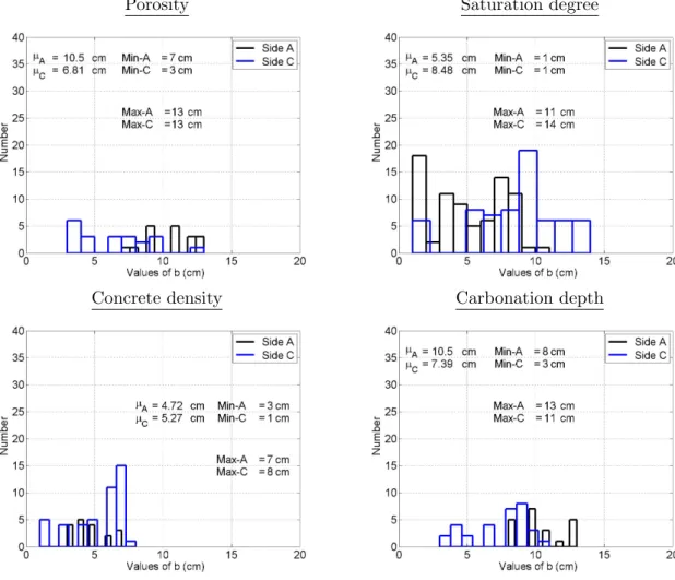
North side (Side A) and 2.42 cm for the South side (Side C). It was therefore decided to consider separately the measurements obtained on each side. In Figure 2 are shown the measured values of porosity, saturation degree, concrete density and carbonation depth for the two exposed sides of the wall. The position of the measurement along the wall is located by its abscissa on the horizontal axis, while the value of the
mea-90
surement of the parameter studied is given on the vertical axis. It is observed that there is a significant spatial variability and that values di↵er for each side.
3. Characterisation of spatial correlation
A trajectory is defined as a successive set of measurements along an horizontal line on the surface of the structure. The set of measurements for each side in Figure 2
95
are examples of trajectories. Given that only one sample path (trajectory) of each random field is available for each side of the wall and for the sake of simplicity, we assume that the random fields are ergodic and Gaussian; this means that one sample (one trajectory of measurements) is sufficient to fully characterise the random field. Otherwise we can carry out as previous step the pre-treatment proposed by (Clerc
and Mallat, 2003). In addition, as well as for many study cases in civil engineering where the amount of data is insufficient (Kenshel, 2009; Li, 2004; O’Connor et al., 2013), we assume second order stationarity. This means that the mean value, the standard deviation are constant, and the autocorrelation function depends only on the distance. The objectives of this section are to describe and illustrate the proposed
105
method called ”windowing” for identifying the range of variation and the mean value of the parameter characterising the autocorrelation function. Section 3.1 provides the basis for the estimation of the parameters that characterise the spatial variability. The proposed windowing method including the criterion to determine the minimum number of points considered in the analysis are described in sections 3.2 and 3.3,
110
respectively. The methodology is finally illustrated in section 3.4.
3.1. Parameters estimation
Let X(x) be a stationary Gaussian random with mean µX, the variance 2X and
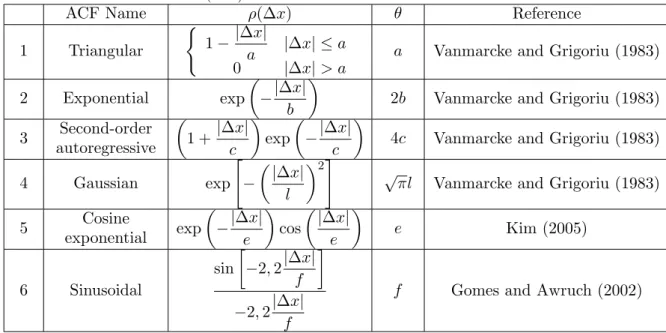
the correlation function ⇢( x). The field X is composed by m spatially correlated positions x1. . . , xm. Many of the correlation functions ⇢( x) (Table 1) were proposed
115
in the literature (see for instance (Der Kiureghian and Ke, 1988; Kenshel, 2009) for an overview). They are characterised by the scale of fluctuation ✓. The scale of fluctuation is related to the distance from which two values from the same random field can be considered more or less dependent from another. Identifying the autocorrelation of a given physical property aims to determine the appropriate type of continuous
120
autocorrelation function and to estimate the corresponding scale of fluctuation ✓. For illustrative purposes, we consider in this work the exponential autocorrelation function, generally used for representing the spatial variability of concrete proper-ties or durability indicators (Kenshel, 2009; Schoefs et al., 2017a, 2016): ⇢( x) = exp( | x| /b) where b = ✓/2. We recall that the correlation matrix R(b) is defined
125
by entries Ri,j(b) = ⇢(xi xj), for i, j = 1, . . . , m. There are two widely used
proce-dures for the estimation of b: Maximum Likelihood Estimation (MLE) and least square (LSM) methods. The LSM is very simple and can be used even for non-Gaussian dis-tributions, it consists in fitting an empirical covariance function ˆC(·) defined in eq. (1) with the parametric model 2X⇢(·).
130 ˆ C(h) = 1 Nh X i (X(xi) µ˜X) (X(xi+ h) µ˜X) , (1) where ˜µX := 1 m m X i=1
X(xi) is the unbiased estimate of µX, Nh being the number of
points distant with h from all locations of study. The fitted parameters from eq. (1) are biased since ˆC is a biased estimator of 2
X⇢(·). The MLE consists in searching for the
value of b that maximises the joint probability density of the data. It gives estimates with minimal variance and asymptotic normal limit. We note ⇣ := (µX, X2, b) and
135
b
⇣ := (ˆµX, ˆX2, ˆb) its estimate by MLE, this later is computed by minimising the negative
log-likelihood (Clerc et al., 2019; Oumouni and Schoefs, 2019), `(⇣, X) = 1 2 ✓ m log( X2) + log|R(b)| + 12 X (X µX)tR(b) 1(X µX) ◆ (2)
where|R(b)| is the determinant of R(b). In practice, an iterative resolution is preferred than direct optimisation procedure. This iterative procedure is summarised by the following steps:
140
(1) we choose an initial estimate ˆb = b0, and we compute its corresponding estimate
of the mean µX and variance 2X, both as follows:
• MLE of the mean µX:
ˆ µX =
X0R(ˆb) 11
10R(ˆb) 11, (3)
where we note by 1 the vector with m entries all equal 1. • MLE of the variance 2
X: 145 ˆ2 = (X µˆX)0R(ˆb) 1(X µˆ X) m (4)
(2) We compute ˆb by minimising ` knowing ˆµX and ˆX2 from step 1.
(3) We repeat these steps until convergence.
This iterative procedure is stopped when two successive estimates ˆb of b are close to a fixed threshold.
3.2. Windowing methodology
150
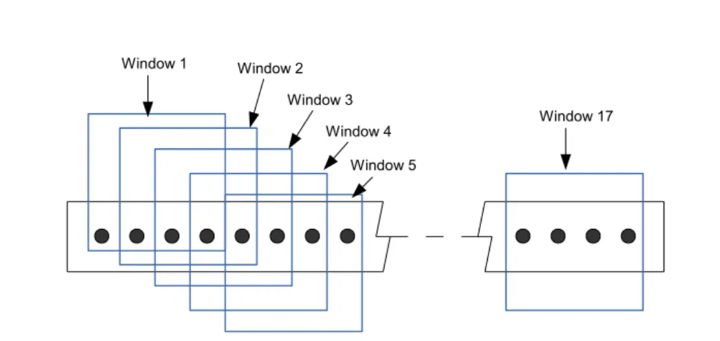
The application of the MLE procedure to a single trajectory will provide only one estimate of ˆb which remains a sample value among other possible values that could be supplied if new trajectories are available. Hence the estimated parameter ˆb can be seen as a random variable whose uncertainty is to be determined. Taking into account that just one trajectory is available in this case and that the measures are correlated for
155
this trajectory, the main focus of the methodology is to identify a range of variation of ˆb as well as its mean value µˆb. Towards this aim, we discretise a trajectory containing N spatial correlated measures into several windows where a value of ˆb is estimated from each the trajectory trapped in the window (Figure 3). Figure 4 summarises the steps of the proposed methodology:
160
(1) Assessment of the minimum number of points per window nw,min: this value is
determined for each trajectory following the procedure detailed in section 3.3. (2) Window definition: we consider a window with a fixed number of successive
measurements nw 2 [nw,min, N ] from which we identify a value of ˆb using the
MLE method (section 3.1).
165
(3) Windowing: we shift the window along the trajectory, and for each position, we identify a new value of ˆb. In Figure 3 are shown various positions of a window containing nw =4 measurements.
(4) Increasing window size: we consider a larger window with nw+ 1 measurements
and we repeat the steps 2 and 3. We increase the length of the window and we
170
repeat the steps 2 and 3 until all measurements are considered (nw= N ).
(5) Post-processing: the identified values of ˆb for nw 2 [nw,min, N ] are considered to
determine the range of variation (minimum and maximum value) as well as the mean of ˆb.
3.3. Assessment of the minimum number of measurements per window
175
It is known from a confidence interval theory that large number of uncorrelated mea-sures allow us to compute a good estimate. However, since there is a considerable correlation between spatial data, the variance of the mean estimate var[ˆµX] stagnates
or decreases very slowly from a given number nm. Therefore, it is possible to define
a minimum number of measures per window nw,min ensuring that var[ˆµX] is close to
180
the value estimated with all values available in the trajectory nw = N .
The minimum number of measurements per window is relatively reached to an accuracy level based on the confidence region of the mean µX. The estimate of µX
given in eq. (3) is unbiased and follows a Gaussian distribution with mean µX and
variance var[ˆµX]. This variance is derived from the inverse of the second derivative of
185 `(⇣, X) with respect to µX: var[ˆµX] = ✓ E @2`(⇣, X) @2µ X ◆ 1 = 2 1R(ˆb) 110. (5)
Therefore, by considering the ↵-quantile of a normal distribution with order ↵, we could define the following confidence interval µX using the estimated value of ˆb:
IµX = 2 4ˆµX q↵ˆX q 10R(ˆb) 11 , ˆµX + q↵ˆX q 10R(ˆb) 11 3 5 , (6)
where ˆX2 is the estimate of 2 defined in eq. (4).
Equation (6) is therefore used to determine nw,mingiven a certain threshold vth> 0
190 as follows: µX := q↵ˆX q 10R(ˆb) 11 ⇡ v th (7)
The minimum number of measurements nw,minfor which the indicator µX satisfies
eq. (7) ensures also that the mean µX respects the following accuracy:
P ✓ ˆ µX 2 [µX vth, µX + vth] ◆ ⇡ 1 ↵. (8)
3.4. Application of the windowing method to the study case
The proposed methodology is illustrated in this section considering the data measured
195
in the side A for the carbonation depth. Following the procedures given in sections 3.2 and 3.3, Figure 5 provides the variance of the mean estimate var[ˆµX] for ↵ = 10% (90%
confidence interval) and various values of nw. It is observed that var[ˆµX] decreases up
to a minimum value of 0.5 when nw = N . For the other trajectories, the minimum
var[ˆµX] varies between 0.4 and 0.5. Taking into account these findings, we selected
200
a threshold value vth = 0.6 to determine nw,min. Table 2 gives the values of nw,min
computed for all the parameters. We found di↵erent values ranging from 8 to 15 for each parameter and side. Since our database is limited to generalise these findings, we
suggest to assess and use a given nw,min per trajectory. The values given in Table 2
will be used in this paper.
205
When carrying out the previous numerical procedure, we obtained for each length of window and each position, a value of ˆb. In Table 3, we provide an example of the assessment of ˆb with the windowing method and measurements of porosity. We observe that when nw varies between 4 and 11, the identification process does not converge
(NC) for some positions of the window. The non-convergence of the MLE method
210
occurs often for windows with fewer number of measurements. Moreover, results in (Rakotovao Ravahatra et al., 2017) showed that for nw <10, statistical uncertainties
in the computation of discrete spatial autocorrelation are significant. For this case we retain the values in green coloured cells that satisfy the condition nw 2 [nw,min, N ].
In Figure 6 are depicted the results of identification of ˆb for all measured parameters
215
and for the two sides (A and C) of the wall. More or less significant di↵erences appear on the mean values of b between the two sides. This can be due to both the e↵ect of degradation and the exposure conditions. Particularly, one observes in Figure 2 that the mean value of porosity and saturation degree are lower and carbonation depth is larger for the side C. This side is south exposed and then prone to exhibit a faster
220
drying of the surface of the concrete, favourable to carbonation. Therefore the data observed are consistent with the process of the degradation. No significant di↵erence is observed for concrete density.
Besides it can be noted in Figure 6 that the values of the mean of ˆb for the concrete density are close on both sides indicating that both faces of the wall are made of the
225
same initial material (the concrete was coming from the same batch when poured and with the same process of concrete vibration). Then it is possible to suggest that the impact of carbonation or exposure conditions on the spatial correlation of concrete density is negligible. The mean values of ˆb for the porosity and carbonation depth are more important on side A than on side C. This can be attributed to the e↵ect of
230
the process of carbonation that is more pronounced on side C and brings additional scatter on the physical properties of the material. This leads hence to less spatial correlation of material properties that are modified by carbonation process (porosity and carbonation depth). The mean of ˆb for the saturation degree is more important on side C than on side A. As this property mainly depends on exposure conditions, a
235
variation between both sides is expected.
According to the previous observations, the spatial autocorrelation of the concrete physical properties that are influenced by carbonation process (porosity and carbon-ation depth) depends on the current deteriorcarbon-ation state driven by carboncarbon-ation. Given these results, we could reasonably conclude that the spatial autocorrelation of
poros-240
ity and carbonation depth changes over time, –i.e. ˆb is a function of time for these parameters. In order to confirm these findings, data collected at several other time steps would be required.
4. Sensitivity of concrete carbonation models to input random fields An optimal maintenance strategy should be supported by models able to predict the
245
corrosion onset caused by concrete carbonation. Given that concrete properties as well as carbonation depth are spatially variable, it is necessary to analyse the ability of models to transfer the spatial correlation of input parameters. We should also assess the influence of each input parameter when it is modelled as a random field. This study extends a previous work (Rakotovao Ravahatra et al., 2017) where the uncertainty on
the assessment of b was not investigated. Since previous results (section 3.4) showed that this uncertainty is significant, we carry out a sensitivity analysis on concrete carbonation models by considering model inputs as independent random fields and varying the value of b. The carbonation models studied in this paper are those which require the physical parameters that are usually investigated in existing structures
255
(porosity, saturation degree, concrete density): Hyvert (2009), Papadakis et al. (1991), Miragliotta (2000) and Ying-Yu and Qui-Dong (1987). According to the review of Rakotovao Ravahatra et al. (2019), we provide a summarised description of these models in Appendix A.
4.1. Methodology
260
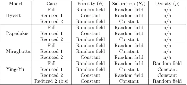
In the first part of the study, we will focus on evaluating separately the influence of considering each model input as a random field. Towards this aim, whereas one input is modelled as a random field, the other inputs are set as deterministic values (mean values). Afterwards, we will consider that all the inputs are represented by random fields (reference case). We summarise in Table 4 the cases studied. The model
265
parameters not mentioned in Table 4 are represented as deterministic values and are provided in Table A3.
The objective being to adopt a wide view and to be able to generalise the results; the sensitivity analysis will consider several values of the autocorrelation parameter (b = 5 cm, 50 cm or 100 cm) for the input parameters modelled as random fields. 5
270
cm appears to be an acceptable minimum with respect to the size of aggregates, 50 cm is close to the distance between two successive points of vibration when pouring concrete, and 100 cm corresponds to the maximum value of b found in the literature (Kenshel, 2009).
The sensitivity analysis concerns the following steps:
275
(1) to generate 100 trajectories (sample paths) for each value of b (5cm, 50cm and 100cm) using the Karhunen-Lo`eve expansion (Karhunen, 1947; Loeve, 1948); (2) to compute the model output (spatial distribution of the carbonation depth at
35 years of exposure) corresponding to the generated input trajectories for the considered carbonation models (Appendix A);
280
(3) to compute the simulated discrete autocorrelation function of the output and to identify the corresponding values of ˆb for the 100 trajectories of carbonation depth using the windowing method described in section 3;
(4) to analyse the e↵ects of the spatial correlation of inputs on the spatial variability of the output (carbonation depth assessed from models).
285
4.2. Results
We present the results in Figures 7, 8, 9 and 10. In these figures are reported results of simulated and empirical discrete autocorrelation, and the histograms of the iden-tified ˆb from the output of the models. On simulated discrete autocorrelation curves, point marks represent the mean values and dotted lines provide the 10% and 90%
290
quantiles values over 100 simulated discrete autocorrelation functions at each x. On the empirical discrete autocorrelation function, points describe the autocorrelation values obtained from measurements and dotted lines provide the bounds determined when uncertainties in measurements and statistical uncertainties are taken into ac-count (Rakotovao Ravahatra et al., 2017). Concerning the histograms of ˆb, we present
on each figure the results corresponding to a given value of b (5 cm, 50 cm and 100 cm) for the input considered. In the following sections, we analyse the results for the cases described in Table 4.
4.2.1. Sensitivity to the porosity random field
We report in Figure 7 the results for each carbonation model when the porosity is
300
modelled as a random field (Case 1 in Table 4).
Regarding simulated discrete autocorrelation functions, the results for all models are similar. When b increases, the gap between minimum and maximum values (scatter) is smaller. One observes hence in the spatial correlation of the models outputs the same tendencies as for the spatial correlation of the porosity. Indeed, when we increase
305
the value of b for the porosity, the realisations of the porosity random field are more correlated and less uncertain. This indicates that the correlation of the porosity is quite well transferred to the model output (simulated carbonation depth).
The ratio of the mean value of ˆb, ˆµb, with respect to the value of b (i.e., ˆµb/b) for
a given input provides a quantification of the ability of the model to transfer spatial
310
correlation from the inputs to the output. We present in Table 5 the ratios ˆµb/b for
each input parameter, each case, and each model.
Regarding porosity (case 1), we can observe that for all models there is an amplifi-cation (ˆµb/b > 1) of the spatial correlation when b50cm. On the contrary there is
a reduction of the spatial dependency when b=100cm. The uncertainties in
measure-315
ments and statistical uncertainties (Rakotovao Ravahatra et al., 2017) could explain these results. Indeed, we can see in Figure 7 (black coloured curves) that these uncer-tainties are quite significant and could have important influence in the identification of ˆb. The presence of uncertainty brings additional difficulties to the analysis and characterisation of the spatial correlation.
320
4.2.2. Sensitivity to the saturation degree random field
We provide in Figure 8 the results for each carbonation model when saturation degree is modelled as a random field (Case 2 in Table 4).
Concerning simulated discrete autocorrelation functions, we can observe significant di↵erences between models. It is difficult to establish a constant value of b over time
325
for the saturation degree because this parameter highly depends on the exposure conditions during the inspection. Nevertheless it can be stated that the mean value of b for this parameter could lie between 5 cm and 50 cm when comparing simulated and empirical discrete autocorrelation functions. This confirms the results in Figure 6. Regarding the model of Ying-Yu, modifying the value of b has no significant impact.
330
Especially, it is observed that between b=50 cm and 100 cm the results are very similar. On the other hand, it is noted that the autocorrelation of the model output is quite low whatever the value of b for the saturation degree. These findings indicate that high correlations of the saturation degree are not transferred to the Ying-Yu model output. The scatter of the simulated discrete autocorrelation is slightly higher for the
335
models of Hyvert and Papadakis and larger than when the porosity is considered as a random filed. These models appear to be more sensitive to saturation random field. We can observe similar trend as for porosity for the model of Miragliotta.
Regarding the histogram of ˆb, we can confirm the same findings observed for the simulated discrete autocorrelation functions. After propagation in the models, the
340
than the one imposed by the porosity. Indeed, we can observe in Table 5 that the ratios ˆ
µb/b for the Case 2 are lower than the Case 1. Concerning the ranges of variation, they
are slightly higher than for Case 1 excepting for the model of Ying-Yu for which it is drastically amplified for b=50cm and b=100cm. These results indicate that excepting
345
the model of Ying-Yu, all the models studied well transfer lower and higher spatial correlation of saturation degree, and are hence sensitive to spatial correlation of this input parameter.
4.2.3. Sensitivity to the concrete density random field
In Figure 9 are reported the results obtained when the concrete density is considered
350
as a random field (Case 3 in Table 4). The results concern only the model of Ying-Yu because it is the only one that uses the concrete density as an input parameter.
Regarding simulated discrete autocorrelation, in comparison with the previous re-sults, one observes that the scatter is larger for b = 5cm. For b = 50 and 100 cm there is an e↵ect on the mean value of the autocorrelation but the scatter is negligible. These
355
findings indicate that Ying-Yu model is highly sensitive to the choice of the value of b used to represent the spatial variability of concrete density.
Concerning the histogram of ˆb, even if there is no scatter in the simulated discrete autocorrelation function when the imposed value of b is equal to 50 cm and 100 cm for density, it is observed an important scatter in the estimated ˆb. On the other hand,
360
the spatial dependency significantly raises after being transferred through the model. Indeed, ˆµb for the simulated carbonation depth is 4 times higher than b when this
latter is equal to 5 cm (Table 5). However, ˆµb/b < 1 when b=100 cm. The same trend
was observed in the previous cases. 4.2.4. Random fields of all inputs
365
In Figure 10 are depicted the results obtained when all the parameters (porosity, saturation degree and density) are modelled as random fields (Case 4 in Table 4).
Concerning simulated discrete autocorrelations, first, we can observe that scatter is wider for the models of Hyvert and Papadakis, while it is smaller for the model of Ying-Yu. The model of Miragliotta is an intermediate between the 2 tendencies.
370
This indicates that some models (Hyvert and Papadakis) are more sensitive to input random fields when compared to others. Second, it is noted that the scatters estimated in Figure 10 are quite similar to those of Figure 8 (random field for saturation degree) for the models of Hyvert, Papadakis and Ying-Yu. This indicates that the spatial variability of the output is highly influenced by the spatial variability of saturation
375
degree for these models. Regarding the Miragliotta model, the scatters when varying b for saturation degree (Figure 8) are wider than when varying it for porosity (Figure 7). However, when varying b for all inputs, the scatters appear to be similar to results in Figure 7 indicating mofe sensitivity to the random field of porosity. This indicates that the Miragliotta model is more sensitive to the spatial variability of the porosity
380
random field. Finally, whatever the correlation of any input of Ying-Yu model, the outputs would always be uncorrelated. Therefore, describing spatial variability with this model appears to be difficult.
Concerning the histogram of ˆb, one observes the same tendencies as with simulated discrete autocorrelation function. Indeed, the histograms are similar to Figure 8 for
385
all models except for the model of Miragliotta which presents the same tendencies as in Figure 7.
We present in Table 6 the Absolute Error (AE) on ˆµb for the Cases 1 to 3. This AE
is estimated taking as a reference the ˆµb of Case 4. The results show that the lowest AE
are for the Case 2 and for the models of Hyvert, Papadakis and Ying-yu. Therefore,
390
the saturation degree appears to be the most influential parameter for these models with respect to spatial correlation propagation. Regarding the model of Miragliotta, the lowest error corresponds to the Case 1. The spatial variability of the output of this model is hence strongly influenced by the spatial variability of the porosity.
Concerning the model of Ying-Yu, the Case 2 leads to similar results than Case 4
395
(see Table 6). This implies that choosing this case will provide simulated carbonation depth with lower spatial correlation. Therefore, the AE analysis is not useful for the Case 2. Following the findings found in Table 5, the Case 1 appears to be better for propagating spatial variability in this model.
The findings of this sensitivity analysis were used to propose the recommendations
400
summarised in Table 7. For instance, it was found that the saturation degree is the most influencing random field for the models of Hyvert and Papadakis. The model of Miragliotta is driven by the spatial variability of the porosity, and the model of Ying-Yu can only deal with the spatial variability of the porosity. The results of this table can be used to define which parameters should be prioritised in inspection campaigns
405
when the objective is to characterise and propagate spatial variability.
5. Evaluation of the recommendations of the sensitivity analysis
In this section we test the previous recommendations (Table 7) to analyse how efficient they are when dealing with the real database obtained during the inspection work presented in Section 2. The following steps are proposed for this study:
410
(1) Define the study cases according to the recommendations given in Table 7. Table 8 provides a description of these study cases. In the full case all the parameters are modelled as random fields. The ”Reduced 1” and ”Reduced 2” cases follow respectively the findings of first (R1) or second (R2) priorities given in Table 7 to determine if the parameters should be modelled as random field or constant
val-415
ues. The constant value is equal to the mean determined from the data reported in Figure 2.
(2) Propagate the spatially correlated data reported in Figure 2 into the carbonation models for each case.
(3) Use the windowing method presented in section 3 to estimate the variability of
420
ˆb for each model and case.
(4) Evaluate the e↵ectiveness of the recommendations by comparing the histograms obtained after propagating spatial variability for each model and case with those estimated from the measurements of carbonation depth (Figure 6). The compar-ison is carried out in terms of the AE between the ˆµb for each model and the ˆµb
425
for measurements (Table 9).
5.1. Full
We present results for all models and for the 2 sides of the wall in the Figure 11. On the side A, we can observe that the models of Hyvert and Ying-Yu appear to underestimate the correlation and provide hence slightly lower values of ˆb. Regarding
430
from measurements. However, no significant di↵erences could be observed between models with respect to side A. On this side, we can also note that the values of ˆb for porosity are low when they are slightly higher for saturation degree (see Figure 6). Excepting the model of Ying-Yu, results of the previous sensitivity analysis show that
435
all models are sensitive to the spatial variability of porosity and saturation degree (see Figures 7 and 8). The e↵ect of slightly higher correlation of porosity appears to be compensated by lower correlation of saturation degree. Consequently we observe the intermediate tendencies on the Figure 11.
Regarding the side C, none of the histograms of ˆb obtained using the models overlaps
440
the one from measurements and di↵erences between models are more important. One observes that the models of Hyvert and Papadakis slightly overestimate ˆb, while the models of Miragliotta and Ying-Yu underestimate it. On the contrary for side A, the identified values of ˆb are lower for porosity in this side, while they are higher for saturation degree (see Figure 6). It appears through these results that the models of
445
Hyvert and Papadakis are more sensitive to higher correlation of saturation degree while the models of Miragliotta and Ying-Yu are more sensitive to lower correlation of porosity. On the other hand, concerning the last two models (Miragliotta and Ying-Yu), the interval of values of ˆb is smaller when compared to the measurements, –i.e. the dispersion is reduced. This is in agreement with the results in Figure 10 where we
450
can see that for these models the transfer of dispersion is lower when compared to the models of Hyvert and Papadakis.
5.2. Reduced 1
Regarding the models of Hyvert and Papadakis, and for the two sides of the wall, the ˆ
µb is close to the results reported in Figure 11. Concerning the models of Miragliotta
455
and Ying-Yu and for the side A, the values of ˆµb in Figure 11 are higher than those
of Figure 12. For the side C, the values of ˆµb are similar to the found for the Full
cases for all the models. In Table 9, it is noted that when considering the Reduced 1 cases, the AE on the assessment of ˆµb are close to the values obtained for the Full
case. These results found when only one random field is propagated in the models
460
may indicate that the recommendations in Table 8 could be sufficient to represent the spatial variability of the problem.
5.3. Reduced 2
Concerning the models of Hyvert and Papadakis and for the side A, one observes that the histograms of ˆb of the model outputs overlap that of the measurements. However,
465
the ranges of variation are widely higher when ˆb is estimated after propagating spatial variability in such models. Regarding the models of Hyvert and Papadakis for the side C and the models of Miragliotta and Ying-Yu for both sides, one observes that the number of identified values of b is small. This is due to a large number of non-convergences found during the simulations. On the other hand, for the model of
Ying-470
Yu and side A, any value of ˆb was identified for the case Reduced 1 (bis). Then, we present in Figure 14 only the results for the side B.
It is noted in Table 9 that the AE are smaller in comparison with the other cases. However, it is not possible to provide a recommendation based on this indicator be-cause: (i) the assessment of ˆµb is based in few data (due to the large number of
475
and minimum bounds when comparing the histograms obtained from measurements and models.
5.4. Summary of recommendations
Previous results highlight that recommendations in Table 7 could be convenient for
480
all models, especially for the models of Hyvert and Papadakis. However, these recom-mendations are less efficient for the models of Miragliotta and Ying-Yu with respect to the side C. This inefficiency could be related to uncertainties in measurements which were more important in side C. The increase of the AE for ˆµb for all models may
indi-cate non negligible correlation between the models inputs, especially for the models of
485
Miragliotta and Ying-Yu. However, in order to confirm this assumption, further data is required.
6. Nugget e↵ects
When analysing auto-covariance, we can observe an abrupt change of the value of the covariance in the beginning of the curve ( x=0). This discontinuity is called
490
“nugget e↵ect” in the field of geostatistics. This may bring additional uncertainty when modelling spatial variability. The nugget e↵ect in variogram analysis was dealt with in some studies (Wagner et al., 2005). Its e↵ect in kriging was also handled by Brooker (1986) or Yin et al. (2011). Concerning the autocorrelation function, we should carry out a similar analysis to the reported in the above-mentioned studies
495
when we observe nuggets in the discrete autocorrelation function. Further work will focus on the development of a methodology to take into account nugget e↵ects in spatial variability assessment.
7. Conclusions and perspectives
The following conclusions are drawn from the present study:
500
• The proposed windowing method is useful for spatial variability characterisation when the spatially correlated data is scarce. It allow us to determine the range of variation and the mean of the parameter used to model the spatial correlation. • Significant di↵erences for the range of variation and mean value of ˆb were found
for each side of the wall for the porosity and carbonation depth. Since
car-505
bonation modifies along time concrete porosity, saturation degree and concrete density, we can suppose that the autocorrelations of these physical properties will also become time-dependent. Further data collected at several time steps is required to confirm this assumption.
• A sensitivity analysis aiming to test the ability of concrete carbonation models
510
to propagate spatial variability was useful to provide recommendations about the input parameters that could be modelled as random fields. This sensitiv-ity analysis was based on simulated data by considering several values of the autocorrelation parameter b.
• The recommendations were tested with the real and scarce database of the case
515
study. This analysis highlighted that the recommendations are rather convenient for all models, especially for the models of Hyvert and Papadakis.
• The proposed methodology and findings of this paper could help to decision-makers to define which parameters are more appropriate to measure and which models are more accurate to use when dealing with spatially deteriorated
prac-520
tical applications. This methodology could be also applied to other deterioration problems.
Further work in this area will focus on:
• Obtaining a more rich spatially correlated database to test the methodology and confirm the findings and assumptions.
525
• Considering correlations between random fields.
• Determining which is the best type of autocorrelation function for each random field.
• Defining which variables should be modelled as random variables. • Adapting the methodology to account for the nugget e↵ect.
530
Acknowledgments
This work was made possible thanks to the French Research Agency ANR ”Build-ing and Sustainable Cities”, which funded the research project ANR-EVADEOS. We are grateful to CEA-Saclay for allowing its installations to be used. Partners of the ANR-EVADEOS project are warmly thanked for the data that have been acquired
535
and shared out (CEA Saclay, IFSTTAR Nantes, LMA Univ. Aix-en-Provence, I2M Univ. Bordeaux, EDF Chatou, LMDC Univ. Toulouse, GeM Univ. Nantes). We also acknowledge the useful comments of the anonymous reviewers to improve the final version of the paper
References
540
Bastidas-Arteaga, E. and Schoefs, F. (2012). “Stochastic improvement of inspection and main-tenance of corroding reinforced concrete structures placed in unsaturated environments.” Engineering Structures, 41, 50–62.
Bastidas-Arteaga, E. and Schoefs, F. (2015). “Sustainable maintenance and repair of RC coastal structures.” Proceedings of the Institution of Civil Engineers - Maritime Engineering,
545
168(4), 162–173.
Brooker, P. I. (1986). “A parametric study of robustness of kriging variance as a function of range and relative nugget e↵ect for a spherical semivariogram.” Mathematical Geology, 18(5), 477–488.
Cameletti, M., Lindgren, F., Simpson, D., and Rue, H. (2012). “Spatio-temporal modeling of
550
particulate matter concentration through the spde approach.” AStA Advances in Statistical Analysis, 97(2), 109–131.
Clerc, M. and Mallat, S. (2003). “Estimating deformations of stationary processes.” The Annals of Statistics, 31(6), 1772–1821.
Clerc, R., Oumouni, M., and Schoefs, F. (2019). “Scap-1d: A spatial correlation assessment
555
procedure from unidimensional discrete data.” Reliab Eng Syst Saf (under revision). Der Kiureghian, A. and Ke, J. (1988). “The stochastic finite element method in structural
reliability.” Prob. Eng. Mech, 3(2), 83–91.
EN-13-791 (2007). Assessment of in-situ compressive strength in structures and pre-cast con-crete components.
560
cor-rosion in concrete structures.” Structural Safety and Reliability : Proceedings of the 7th international conference on structural safety and reliability, 435–442.
Gomes, H. M. and Awruch, A. M. (2002). “Reliability of reinforced concrete structures using stochastic finite elements..” Engineering Computations, 19(7-8), 764–786.
565
Gomez-Cardenas, C., Sbarta, M., Garnier, V., and Balayssac, J. (2015). “NDT inspection strategy to minimize the number of samples for onsite concrete evaluation.” Proceedings of Int. Symp. on NDT-CE, Berlin, Germany (15-17 September).
Hyvert, N. (2009). “Application de l’approche probabiliste de la durabilit´e des produits pr´efabriqu´es en b´eton.” PhD thesis, Universit´e de Toulouse III-Paul Sabatier, Universit´e
570
de Toulouse III-Paul Sabatier.
Karhunen, K. (1947). “Uber lineare methoden in der wahrscheinlichkeitsrechnung.” Amer. Acad. Sci, 37, 3–79.
Karimi, A., Ramachandran, K., and Buenfeld, N. R. (2005). “Probabilistic analysis of re-inforcement corrosion with spatial variability.” 9th International Conference on Structural
575
Safety and Reliability, ICOSSAR’05, Millpress, Rotterdam.
Kenshel, O. M. (2009). “Iinfluence of spatial variability ofn whole life management of reinforced concrete bridges.” Ph.D. thesis, University of Dublin, Trinity college, University of Dublin, Trinity college.
Kim, H. (2005). “Spatial variability in soils: Sti↵ness and strength.” Ph.D. thesis, Georgia
580
Institute of Technology, Georgia.
Li, C. Q. (2004). “Reliability based service life prediction of corrosion a↵ected concrete struc-tures..” Ph.D. thesis, Delft University, Netherlands.
Lindgren, F., Rue, H., and Lindstrm, J. “An explicit link between gaussian fields and gaussian markov random fields: the stochastic partial di↵erential equation approach.” Journal of the
585
Royal Statistical Society: Series B (Statistical Methodology), 73(4), 423–498.
Loeve, M. (1948). Fonctions al´eatoires du second ordre. Gautiers Villars, Paris Supplement to P. Levy, “Processus stochastic et mouvement Brownien”.
Miragliotta, R. (2000). “Mod´elisation des processus physico-chimiques de la carbonatation des b´etons pr´efabriqu´es - prise en comptes des e↵ets de paroi.” Ph.D. thesis, Universit´e de la
590
Rochelle, Universit´e de la Rochelle.
Moshtaghin, A. F., Franke, S., Keller, T., and Vassilopoulos, A. P. (2017). “Experi-mental characterization of longitudinal mechanical properties of clear timber: Random spatial variability and size e↵ects.” Construction and Building Materials, 120, 432–441 https://doi.org/10.1016/j.conbuildmat.2016.05.109.
595
NF-18-459 (2010). Concrete - Testing hardened concrete - Testing porosity and density. O’Connor, A., Sheils, E., Breysse, D., and Schoefs, F. (2013). “Markovian bridge maintenance
planning incorporating corrosion initiation and non-linear deterioration.” ASCE journal of bridge engineering, 3, 189–199.
Othmen, I., Bonnet, S., and Schoefs, F. (2018). “Statistical investigation of di↵erent
analy-600
sis methods for chloride profiles within a real structure in a marine environment.” Ocean Engineering, 157(1), 96–107.
Oumouni, M. and Schoefs, F. (2019). “An adaptive approach for spatial variability assessment of structures from distributed measurements.” Reliab Eng Syst Saf (under review).
Papadakis, V., Vayenas, C., and Fardis, M. (1991). “Fundamental modelling and experimental
605
investigation of concrete carbonation.” ACI Materials Journal, 4(88), 363–373.
Rakotovao Ravahatra, N., Bastidas-Arteaga, E., Schoefs, F., de Larrard, T., and Duprat, F. (2019). “Probabilistic and sensitivity analysis of analytical models of corrosion onset for reinforced concrete structures.” European Journal of Environmental and Civil Engineering https://doi.org/10.1080/19648189.2019.1591307.
610
Rakotovao Ravahatra, N., Schoefs, F., Duprat, F., de Larrard, T., and Bastidas-Arteaga, E. (2017). “Assessing the capability of analytical carbonation models to propagate uncertainties and spatial variability of reinforced concrete structures.” Frontiers in Built Environment: Bridge Engineering, 3(1), 1–9.
Schmitt, G. (2009). Global needs for knowledge dissemination, research, and development in
materials deterioration and corrosion control. The World Corrosion Organization, New York, NY.
Schoefs, F., Bastidas-Arteaga, E., and Tran, T. (2017a). “Optimal embedded sensor placement for spatial variability assessment of stationary random fields.” Engineering Structures, 17, 35–44.
620
Schoefs, F., Bastidas-Arteaga, E., Tran, T., Villain, G., and Derobert, X. (2016). “Character-ization of random fields from NDT measurements: A two stages procedure.” Engineering structures, 111, 312–322 https://doi.org/10.1016/j.engstruct.2015.11.041.
Schoefs, F., Oumouni, M., Clerc, R., Othmen, I., and Bonnet, S. (2017b). “Statistical analysis and probabilistic modeling of chloride ingress spatial variability in concrete coastal
infras-625
tructures.” EDITION 4, SPLIT, Croatia, Coastal and Maritime Mediterranean Conference. Stewart, M. (2006). “Spatial variability of damage and expected maintenance costs for deterio-rating rc structures.” Structure and Infrastructure Engineering: Maintenance, Management, Life-Cycle Design and Performance, 2(2), 70–90.
Stewart, M. and Mullard, J. (2007). “Spatial time-dependent reliability analysis of corrosion
630
damage and the timing of first repair for RC structures.” Engineering structures, 29, 1457– 1464.
Tesfamariam, S., Bastidas-Arteaga, E., and Lounis, Z. (2018). “Seismic Retrofit Screen-ing of ExistScreen-ing Highway Bridges With Consideration of Chloride-Induced Deterioration: A Bayesian Belief Network Model.” Frontiers in Built Environment, 4, 1–11.
635
Torres-Luque, M., Bastidas-Arteaga, E., Schoefs, F., Sanchez-Silva, M., and Osma, J. (2014). “Non-destructive methods for measuring chloride ingress into concrete: State-of-the-art and future challenges.” Construction and Building Materials, 68, 68–81 https://doi.org/10.1016/j.conbuildmat.2014.06.009.
Torres-Luque, M., Osma, J., Sanchez-Silva, M., Bastidas-Arteaga, E., and Schoefs, F. (2017).
640
“Chlordetect: Commercial calcium aluminate based conductimetric sensor for chloride pres-ence detection.” Sensors, 17, 1–19.
Vanmarcke, E.-H. and Grigoriu, M. (1983). “Stochastic finite element analysis of simple beams.” J. Eng. Mech., 109(5), 1203–1214.
Villain, G., Balayssac, J., and Garnier, V. (2017). Non-destructive Testing and Evaluation of
645
Civil Engineering Structures. ISTE Press - Elsevier, 1st edition, Chapter 9, 1st edition. Wagner, H. H., Holderegger, R., Werth, S., Gugerli, F., Hoebee, S. E., and Scheidegger,
C. (2005). “Variogram analysis of the spatial genetic structure of continuous popula-tions using multilocus microsatellite data.” Genetics, 169(3), 1739?1752 doi: 10.1534/ge-netics.104.036038.
650
Wang, H., Wang, X., Wellmann, J. F., and Liang, R. Y. (2018). “Bayesian stochastic soil modeling framework using gaussian markov random fields.” ASCE-ASME Journal of Risk and Uncertainty in Engineering Systems, Part A: Civil Engineering, 4(2), 04018014. Yin, J., Ng, S., and Ng, K. (2011). “Kriging metamodel with modified nugget-e↵ect: The
heteroscedastic variance case.” Computers & Industrial Engineering, 61, 760–777.
655
Ying-Yu, L. and Qui-Dong, W. (1987). “The mechanism of carbonation of mortars and the dependence of carbonation on pore structure.” ACI-SP 100, Concrete Durability, 1915–1943. Zhu, F., Zhou, Q., Wanga, F., and Yang, X. (2017). “Spatial variability and sensitivity analysis on the compressive strength of hollow concrete block masonry wallettes.” Construction and Building Materials, 140, 129–138 https://doi.org/10.1016/j.conbuildmat.2017.02.099.
Table 1. Autocorrelation function (ACF) and scale of fluctuations
ACF Name ⇢( x) ✓ Reference
1 Triangular
(
1 | x|
a | x| a 0 | x| > a
a Vanmarcke and Grigoriu (1983)
2 Exponential exp
✓ | x|
b ◆
2b Vanmarcke and Grigoriu (1983) 3 Second-order autoregressive ✓ 1 +| x| c ◆ exp ✓ | x| c ◆
4c Vanmarcke and Grigoriu (1983)
4 Gaussian exp " ✓ | x| l ◆2# p
⇡l Vanmarcke and Grigoriu (1983)
5 Cosine exponential exp ✓ | x| e ◆ cos ✓ | x| e ◆ e Kim (2005) 6 Sinusoidal sin 2, 2| x| f 2, 2| x| f
f Gomes and Awruch (2002)
Table 2. Values of nw,minfor the studied parameters
Parameter nw,min for Side A nw,min for Side B
Porosity 15 8
Saturation 9 10
Density 8 12
Table 3. Identified values of b(cm) for porosity (Side A), each nw and each position of the window
nw 1 2 3 4 5 Position of the corresponding window6 7 8 9 10 11 12 13 14 15 16 17
4 8 16 7 8 18 12 NC NC NC NC NC NC NC 12 NC 12 16 5 24 11 9 13 17 NC NC NC NC NC NC NC NC NC 11 19 – 6 20 10 14 13 11 NC NC NC NC NC NC NC NC 11 17 – – 7 13 14 13 10 11 NC NC NC NC NC 6 NC 9 16 – – – 8 16 13 10 10 8 NC NC NC NC NC NC 7 16 – – – – 9 15 10 10 8 7 NC NC NC NC NC 8 13 – – – – – 10 10 10 8 7 7 NC NC NC NC 6 14 – – – – – – 11 10 8 7 7 8 NC NC NC 6 12 – – – – – – – 12 8 7 7 8 10 6 6 6 12 – – – – – – – – 13 7 7 8 10 11 10 6 12 – – – – – – – – – 14 7 8 10 11 7 7 11 – – – – – – – – – – 15 8 10 11 8 10 12 – – – – – – – – – – – 16 10 11 8 10 13 – – – – – – – – – – – – 17 11 8 10 13 – – – – – – – – – – – – – 18 8 10 13 – – – – – – – – – – – – – – 19 10 13 – – – – – – – – – – – – – – – 20 13 – – – – – – – – – – – – – – – – NC: non convergence
Table 4. Summary of cases for the sensitivity analysis
Case Model Porosity ( ) Saturation (Sr) Density (⇢) Results
1 Hyvert Random field Constant n/a
Figure 7
Papadakis Random field Constant n/a
Miragliotta Random field Constant n/a
Ying-Yu Random field Constant Constant
2 Hyvert Constant Random field n/a
Figure 8
Papadakis Constant Random field n/a
Miragliotta Constant Random field n/a
Ying-Yu Constant Random field Constant
3 Ying-Yu Constant Constant Random field Figure 9
4 Hyvert Random field Random field n/a
Figure 10 Papadakis Random field Random field n/a
Miragliotta Random field Random field n/a Ying-Yu Random field Random field Random field
Table 5. Ratio ˆµb/b for the each model and cases
Hyvert Papadakis Miragliotta Ying-Yu
b (cm) µˆb (cm) µˆb/b µˆb (cm) µˆb/b µˆb (cm) µˆb/b µˆb (cm) µˆb/b Case 1 5 9.09 1.81 9.09 1.81 8.77 1.75 9.1 1.82 50 69.2 1.38 67.9 1.35 67.6 1.35 71.9 1.43 100 64.2 0.64 62.9 0.62 62.7 0.62 66.7 0.66 Case 2 5 9.04 1.8 9.02 1.8 9.03 1.8 9.07 1.81 50 39.8 0.79 41.9 0.83 60.2 1.2 41.1 0.82 100 49 0.49 52.5 0.52 63.5 0.63 39.5 0.39 Case3
5 n/a - n/a - n/a - 20.7 4.14
50 n/a - n/a - n/a - 93.1 1.86
100 n/a - n/a - n/a - 78.1 0.78
Case 4
5 9.09 1.81 9.11 1.82 9.13 1.82 8.91 1.78
50 40.1 0.8 45.4 0.9 65.5 1.31 42 0.84
100 48.2 0.48 51.7 0.51 60.2 0.6 40.2 0.4
n/a: non applicable
Table 6. Absolute Error (AE) on the mean of ˆb between the Case 4 and all other cases
Hyvert Papadakis Miragliotta Ying-Yu
b (cm) µˆb (cm) AE (%) µˆb (cm) AE (%) µˆb (cm) AE (%) µˆb (cm) AE (%) Case 1 5 9.09 0 9.09 -0.21 8.77 -3.94 9.1 2.13 50 69.2 72.56 67.9 49.55 67.6 3.2 71.9 71.19 100 64.2 33.19 62.9 21.66 62.7 4.15 66.7 65.92 Case 2 5 9.04 -0.55 9.02 -0.98 9.03 -1.09 9.07 1.79 50 39.8 -0.74 41.9 -7.7 60.2 -8.09 41.1 -2.14 100 49 1.65 52.5 1.54 63.5 5.48 39.5 -1.74 Case 3
5 n/a - n/a - n/a - 20.7 132.32
50 n/a - n/a - n/a - 93.1 121.66
100 n/a - n/a - n/a - 78.1 94.27
n/a: non applicable
Table 7. Recommendations about modelling input parameters as random fields for each model
Model Porosity ( ) Saturation (Sr) Density (⇢)
Hyvert R2 R1 n/a
Papadakis R2 R1 n/a
Miragliotta R1 R2 n/a
Ying-Yu R1 NR NR
R1: recommended (priority), R2: recommended (second priority), NR: non recommended, n/a: non applicable
Table 8. Summary of study cases for evaluating the recommendations obtained from numerical analysis
Model Case Porosity ( ) Saturation (Sr) Density (⇢)
Hyvert
Full Random field Random field n/a
Reduced 1 Constant Random field n/a
Reduced 2 Random field Constant n/a
Papadakis
Full Random field Random field n/a
Reduced 1 Constant Random field n/a
Reduced 2 Random field Constant n/a
Miragliotta
Full Random field Random field n/a
Reduced 1 Random field Constant n/a
Reduced 2 Constant Random field n/a
Ying-Yu
Full Random field Random field Random field
Reduced 1 Random field Constant Constant
Reduced 2 Constant Random field Constant
Reduced 2 (bis) Constant Constant Random field
n/a: non applicable
Table 9. Absolute error (AE) between ˆµbcomputed from the models and ˆµbestimated from the data
Side A Side C
Case µˆb (cm) AE (%) µˆb (cm) AE (%)
Measurements n/a 10.35 n/a 7.39 n/a
Hyvert Full 7.19 31 9.47 28 Reduced 1 6.57 37 9.5 28 Reduced 2 12 14 8.45 14 Papadakis Full 7.89 24 9.12 23 Reduced 1 6.63 36 9.64 30 Reduced 2 12 14 8.07 9 Miragliotta Full 9.18 12 5.62 23 Reduced 1 12.4 18 4.83 34 Reduced 2 10.6 0 6.24 15 Ying-Yu Full 7.21 31 5.33 27 Reduced 1 12.4 18 5.47 25 Reduced 2 10.8 2 6.71 9 Reduced 2 (bis) NC – 6.3 14
Figure 1. Studied wall
Window 1 Window 2 Window 3
Window 4 Window 5
Window 17
Spatially distributed data
Determination of the minimum number of points per window nw,min
Place the initial window at the left (or rigth) extremity
Identify b Window at the rigth (or left) extremity ? Shift window i = i + 1 nw > N END
Bounds and mean of b
No Yes
Yes
No
Figure 5. Variance of the mean estimate var[ˆµX] for the carbonation data of side A
Porosity Saturation degree
Concrete density Carbonation depth
Discrete autocorrelation Identified values of ˆb
Discrete autocorrelation Identified values of ˆb
Discrete autocorrelation Identified values of ˆb
Discrete autocorrelation Identified values of ˆb
Figure 11. Correspondence between identified values of ˆb from models outputs and measurements for Full cases
Figure 12. Correspondence between identified values of ˆb from models outputs and measurements for Reduced 1 cases
Figure 13. Correspondence between identified values of ˆb from models outputs and measurements for Reduced 2 cases
Figure 14. Supplementary correspondence between identified values of ˆb from models outputs and measure-ments for Reduced 2 bis case and the model of Ying-Yu
Appendix A. Models
According to (Rakotovao Ravahatra et al., 2019), concrete carbonation models can be written in a generalized expression:
x(t) =pkexpkexekPDCO2
p
t (A1)
where x(t) [m] is the carbonation depth at time t [s], kexp is a factor which introduces
environmental conditions, kexe is a factor accounting for execution conditions, kP is
665
a factor accounting for the interaction between the di↵usion coefficient of the carbon dioxide DCO2 [m
2/s] and the concrete porosity . k
P is expressed as:
kP = kP,MkP,E (A2)
where kP,M is related to material properties and kP,E to exposure conditions.
Expres-sions of kP,M, kP,E, kexp and kexe are given in Table A1 for each considered model.
↵1 and n1 are fitting parameters, fp is the volumetric fraction of the cement paste,
670
R is the gas constant (8.31 USI), RH is Relative humidity, T is temperature, PCO2
is carbon dioxide pressure, is porosity, Sr is saturation degree, ⇢ is concrete
den-sity, [Component] is the “component” content, Cabs is the absorbed carbone dioxide
(Cabs= (1 Sr)⇥ C0) , C0 is the CO2 content at the exposed surface, keis a
param-eter which assesses environmental conditions, kc is a parameter which considers cure
675 conditions. ke= 0 B @ 1 RH 100 2.5 1 ⇣RHref 100 ⌘2.5 1 C A 5 (A3)
where RHref corresponds to a reference relative humidity ('65%). HR could be
com-puted using Sr from desorption curves.
Despite the fact that cement paste hydrates and unhydrates contents are input parameters for the same models, it was decided to consider their variability through
680
hydration degree ↵hyd and cement content c, using the empirical expressions, found
in Hyvert (2009). The mean value of measured compressive strength is 40 MPa. This value is similar to C45 concrete. Therefore, we assume a cement content equal to c =350 kg/m3. Table A2 presents a cement composition which could suit for such a concrete. The values of the other parameters are given in Table A3.
Ta b le A 1 . Expr es si ons of kP, E , kP, M , kex p and kex e Mo d el kP, E kP, M DCO 2 kex p kex e Yi n g -Y u a n d Qu i-D o n g (1 9 8 7 ) 2 PCO 2 / (C abs ⇢ ) 1 DYu =e x p (1 0 5 .66 0 .877) 1 1 Pa p a d a k is et a l. (1 9 9 1 ) C0 2 / ([ CH ]+3 [CS H ]+3 [C 3 S ]+2 [C 2 S ]) DPa =1 .64 ⇥ 10 6f 1 .8 p (1 RH) 2 .2 1 1 Mi ra g li o tt a (2 0 0 0 ) C0 2(1 Sr )(1 ) 1([ CH ]+3 [CS H ]+3 [C 3 S ] D a 1 1 +2[ C2 S ]+4 [C 4 AF ]+3 [C 3 A ]) 1 1 Hyv er t (2 0 0 9 ) 2 PCO 2 R T f 1 p ⇣ [CH ]+4 [AF t]+3 [AF m ]+ 1 .65[ CS H ] n1 +1 ⇣P CO 2 Patm ⌘n 1 ⌘ 1 D ke kc ⇥ ⇣ 1+ ↵1 1 .65[ CS H ] ⇣P CO 2 Patm ⌘n 1 ⌘ 1 aD could b e measured through destructiv e testing or calcul a ted using prev ious empirical ex pressions, in this wo rk DPa is used
Table A2. Cement composition (%) Component (%) SiO2 20.1 Al2O3 5 Fe2O3 3 CaO 64.1 MgO 1 SO3 3.2 K2O 0.72
Table A3. Values of input parameters for carbonation models
Parameter Unit Value
RH % 72.91 kc - 0.63 kt - 0.98 T K 284.04 c kg/m3 350 ↵hyd 0.81 Patm Pa 101325 PCO2 Pa 40.53 C0 kg/m3 6.5⇥10 4 ↵1 L/mol 23.5 n1 - 0.67