Network pricing problems : complexity, polyhedral study and solution approaches

AVIS

Ce document a été numérisé par la Division de la gestion des documents et des archives de l’Université de Montréal.

L’auteur a autorisé l’Université de Montréal à reproduire et diffuser, en totalité ou en partie, par quelque moyen que ce soit et sur quelque support que ce soit, et exclusivement à des fins non lucratives d’enseignement et de recherche, des copies de ce mémoire ou de cette thèse.

L’auteur et les coauteurs le cas échéant conservent la propriété du droit d’auteur et des droits moraux qui protègent ce document. Ni la thèse ou le mémoire, ni des extraits substantiels de ce document, ne doivent être imprimés ou autrement reproduits sans l’autorisation de l’auteur.

Afin de se conformer à la Loi canadienne sur la protection des renseignements personnels, quelques formulaires secondaires, coordonnées ou signatures intégrées au texte ont pu être enlevés de ce document. Bien que cela ait pu affecter la pagination, il n’y a aucun contenu manquant.

NOTICE

This document was digitized by the Records Management & Archives Division of Université de Montréal.

The author of this thesis or dissertation has granted a nonexclusive license allowing Université de Montréal to reproduce and publish the document, in part or in whole, and in any format, solely for noncommercial educational and research purposes.

The author and co-authors if applicable retain copyright ownership and moral rights in this document. Neither the whole thesis or dissertation, nor substantial extracts from it, may be printed or otherwise reproduced without the author’s permission.

In compliance with the Canadian Privacy Act some supporting forms, contact information or signatures may have been removed from the document. While this may affect the document page count, it does not represent any loss of content from the document.

Faculté des Sciences

Université Libre de Bruxelles

Département d'informatique et de recherche opérationnelle Faculté des Arts et des Sciences

Université de Montréal

Network pricing problems: complexity, polyhedral study and solution approaches

par

Géraldine Heilporn (boursière du F.R.I.A.)

Thèse présentée en vue de l'obtention du grade de Ph.D. en informatique (UdeM)

Docteur en Sciences (ULB)

Oétobre, 2008

Faculté des études supérieures

Cette thèse intitulée:

Network pricing problems: complexity, polyhedral study and solution approaches

présentée par: Géraldine Heilporn

a été évaluée par un jury composé des personnes suivantes: Bernard Gendron,

Patrice Marcotte, Gilles Savard, Martine Labbé, Michel Gendreau, Stan van Hoesel,

président-rapporteur

directeur de recherche U deM codirecteur U deM

directeur de recherche ULB membre du jury

Considérons le problème qui consiste à maximiser les profits issus de la tarification d'un sous-ensemble d'arcs d'un réseau de transport, où les flots origine-destination (produits) sont affectés aux plus courts chemins par rapport aux tarifs et aux coûts initiaux. Cette thèse porte sur une structure de réseau particulière du problème ci-dessus, dans laquelle tous les arcs tarifables sont connectés et forment un chemin, comme c'est le cas sur une autoroute. Étant donné que les tarifs sont habituellement déterminés selon les points d'entrée et de sortie sur l'autoroute, nous considérons un graphe tarifable complet, où chaque arc correspond en réalité à un sous-chemin. Deux variantes de ce problème sont étudiées, avec ou sans contraintes spécifiques reliant les niveaux de tarifs sur les arcs.

Ce problème peut être modélisé comme un programme linéaire mixte entier. Nous prouvons qu'il est Np-difficile. Plusieurs familles d'inégalités valides sont ensuite proposées, celles-ci renforçant certaines contraintes du modèle initial. Leur efficacité est d'abord démontrée de manière théorique, puisqu'il s'agit de facettes des problèmes restreints à un ou deux produits. Certaines des inégalités valides proposées, ainsi que plusieurs contraintes du modèle initial, permettent aussi de donner une description complète de l'enveloppe convexe des solutions réalisables d'un problème restreint à un seul produit. Des tests numériques ont également été menés, et mettent en évidence l'efficacité réelle des inégalités valides pour le problème général à plusieurs produits. Enfin, nous soulignons les liens entre le problème de tarification de réseau étudié dans cette thèse et un problème plus classique de tarification de produits en gestion.

Mots clés: Tarification de réseaux, programmation mixte entière, op-timisation combinatoire.

Consider the problem of maximizing the revenue generated by tolls set on a subset of arcs of a transportation network, where origin-destination flows (commodi ties) are assigned to shortest paths with respect to the sum of tolls and initial costs. This thesis is concerned with a particular case of the above problem, in which all toll arcs are connected and constitute a path, as occurs on highways. Further, as tollieveis are usually computed using the highway entry and exit points, a complete toll subgraph is considered, where each toll arc corresponds to atoll subpath. Two variants of the problem are studied, with or without specifie constraints linking together the tolls on the arcs.

The problem is modelled as a linear mixed integer program, and proved to be NP-hard. Next, several classes of valid inequalities are proposed, which strengthen important constraints of the initial model. Their efficiency is first shown theoreti-cally, as these are facet defining for the restricted one and two commodity problems. Also, we prove that sorne of the valid inequalities proposed, together with sever al constraints of the linear program, provide a complete description of the convex hull of feasible solutions for a single commodity problem. Numerical tests have also been conducted, and highlight the practical efficiency of the valid inequalities for the multi-commodity case. Finally, we point out the links between the problem studied in the thesis and a more classical design and pricing problem in economics. Keywords: Network pricing, mixed-integer programming, combina-torial optimization.

RÉSUMÉ III

ABSTRACT IV

CONTENTS . . . . V

LIST OF TABLES. Vlli

LIST OF FIGURES. Xl

LIST OF APPENDICES. Xill

LIST OF ABBREVIATIONS XIV

NOTATION . . . .. xv

ACKNOWLEDGMENTS

CHAPTER 1: INTRODUCTION

CHAPTER 2: THE NETWORK PRICING PROBLEM 2.1 Bilevel programming . . . .

2.2 (Bi)linear bilevel programming . 2.3 The Network Pricing Problem .

CHAPTER 3: NETWORK PRICING WITH CONNECTED TOLL ARCS . . . .

3.1 Network Pricing Problems with Connected ToU Arcs 3.2 Model reformulation 3.3 Preprocessing . . . . xvi 1 5 5 8 13 23 23 30 32

3.4 Setting the constants M and N 3.5 Complexity . . . .

CHAPTER 4: VALID INEQU ALITIES . 4.1 Strengthening the Shortest Path Inequalities 4.2 Strengthening the Profit Upper Bound Inequalities 4.3 Extension . 4.4 Conclusion. 33 34 43 44

47

56 57

CHAPTER 5: ASSESSING THE VALID INEQUALITIES 58

5.1 Single commodity Problems . . . 58

5.1.1 Single commodity CCT-NPP 58

5.1.2 Single commodity GCT-NPP 68

5.2 Two-commodity problems 5.3 Conclusion . . . .

CHAPTER 6: NUMERICAL RESULTS 6.1 Data instances. . . .

6.2 Implementation of models

6.3 Numerical results for GCT-NPP . 6.3.1

6.3.2 6.3.3

Strengthened Shortest Path inequalities .

Strengthened Profit Upper Bounds inequalities . Final tests for (HP3) ..

6.4 Numerical results for CCT-NPP

6.4.1 Strengthened Shortest Path inequalities . 6.4.2 Strengthened Profit Upper Bound Inequalities 6.4.3 Final tests for (HP3*)

6.5 Conclusion... 71 105 106 106 108

110

110

114

117

120 120 124 126 129

CHAPTER 7: LINKING PRICING PROBLEMS IN

TRANSPORTA-TION NETWORKS AND ECONOMICS 130

7.1

Designing and pricing a set of products

130

7.1.1

Problern definition

131

7.1.2

Literature review

133

7.1.3

Profit and Bundle Pricing Problerns .

136

7.2

Relationships between both farnilies of problerns

145

7.2.1

Seller Welfare, Profit Problerns and GCT-NPP .

145

7.2.2

Bundle Pricing and Network Pricing Problern

147

7.3

Cornparison between a Modified Profit Problern and the GCT-NPP

148

7.4 Conclusion...

154

CHAPTER 8: CONCLUSION 155

3.1 Fixed costs c~ : k = kl , k2 , a E A for a network example with three entry /exit nodes on the highway . . . .

6.1 Number of feasible paths per commodity 6.2 Model (HP3) . . . .. 6.3 Model (HP3) with inequalities (4.1)

6.4 Number of inequalities (4.1) appended to (HP3) 6.5 Model (HP3) with inequalities (4.2) . . . . . . 6.6 Number of inequalities (4.2) appended to (HP3) 6.7 Model (HP3) with inequalities (4.1) and (4.2) . 6.8 Number of inequalities (4.1)-(4.2) appended to (HP3)

28 108 110 111 111 111 111 113 113 6.9 Model (HP3) with inequalities (4.1) and (4.2) appended only at root 113 6.10 Model (HP3) with inequalities (4.7)-(4.8) . . . 114 6.11 Number of inequalities (4.7)-(4.8) appended to (HP3) 114 6.12 Model (HP3) with inequalities (4.9)-(4.10) . . . 115 6.13 Number of inequalities (4.9)-(4.10) appended to (HP3) 115 6.14 Model (HP3) with inequalities (4.11) . . . 115 6.15 Number of inequalities (4.11) appended to (HP3) 115 6.16 Model (HP3) with inequalities (4.7)-(4.8) and (4.9)-(4.10) 116 6.17 Model (HP3) with inequalities (4.7)-(4.8) and (4.11) 116 6.18 Model (HP3) with inequalities (4.9)-(4.10) and (4.11) 117 6.19 Model (HP3) withinequalities (4.1)-(4.2), (4.7)-(4.8) and (4.9)-(4.10)

(only at root) . 118

6.20 Model (HP3*) 120

6.21 Model (HP3*) with inequalities (4.1) 121

6.23 Madel (HP3*) with inequalities (4.2) . . . . 6.24 Number of inequalities (4.2) appended ta (HP3*) 6.25 Madel (HP3*) with inequalities (4.1) and (4.2)

6.26 Number of inequalities (4.1)-(4.2) appended ta (HP3*)

121 121 122 122 6.27 Madel (HP3*) with (4.1) and (4.2) inequalities appended only at root 123 6.28 Madel (HP3*) with inequalities (4.7)-(4.8) . . . 124 6.29 Number of inequalities (4.7)-(4.8) appended ta (HP3*) 124 6.30 Madel (HP3*) with inequalities (4.9)-(4.10) . . . 124 6.31 Number of inequalities (4.9)-(4.10) appended ta (HP3*) 125 6.32 Madel (HP3*) with inequalities (4.11) . . . 125 6.33 Number of inequalities (4.11) appended ta (HP3*) 125 6.34 Madel (HP3*) with inequalities (4.7)-(4.8) and (4.9)-(4.10) 126 6.35 Madel (HP3*) with inequalities (4.1)-(4.2), (4.7)-(4.8) and

(4.9)-(4.10) (only at root) . . . 127 6.36 Madel (HP3*) with inequalities (4.1)-(4.2) and (4.7)-(4.8) (only at

root) 127

7.1 Links between notations for the :Modified Profit Problem and the General Complete Toll NPP . . . 146 7.2 Madel (LMPP) with (7.21), (7.22) and (7.23) inequalities . 150 7.3 Madel (HP3*) with (7.21), (7.22) and (7.23) inequalities 151 7.4 Madel (LMPP) with (7.21), (7.22) and (7.23) inequalities, tested on

Shioda et al. instances . . . . . ~ . . . . . . . . .

. . .

.

. .

. 152 7.5 :Madel (HP3*) with (7.21), (7.22) and (7.23) inequalities, tested on

Shioda et al. instances . . . 152 7.6 Madel (HP3*) with (4.1)-(4.2), (4.7)-(4.8) and (4.9)-(4.10)

7.7 Madel (HP3*) with (4.1)-(4.2), (4.7)-(4.8), (4.9)-(4.10), (7.21), (7.22) and (7.23) inequalities, tested on Shioda et al. instances . . . 154

2.1 Evolution of the objective function tXl with respect to tax t

2.2 Network example . . . . . . . 2.3 Main contributions to the Network Pricing Problem

12 14 22

3.1 Basic NPP . . . 24

3.2 Complete Toll NPP 25

3.3 Optimal tolls

ta :

a E A for a network example with three entry jexit nodes on the highway . . . 28 3.4 Subnetworks on which Triangle and Monotonicity constraints apply 29 3.5 Example of a toll arc b ECa . . . . . . . . 33

3.6 Subnetwork for variable Xi (single directional Constrained Complete Toll NPP).

3.7 Part of network for F = ( ... V Xi V Xj) 1\ (Xj V Xz V ... ) 1\ ... (single directional Constrained Complete Toll NPP).

3.8 Subnetwork for variable Xi.

3.9 Subnetwork for F = ( ... V Xi V Xj) 1\ (Xj V Xz V ... ) 1\ ... (bi-directional Constrained Complete Toll NPP).

3.10 Subnetwork for variable Xi (All feasible access Constrained Complete Toll NPP) . . . .

5.1 Examples of b EC_a and b E Ca

5.2 Part of network for the assumption of Proposition 29

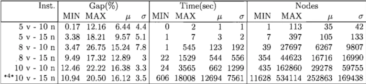
6.1 Evolution of the objective function with respect to the cpu time for an instance of class 8v-lOn

6.2 Evolution of the objective function with respect to the cpu time for 36 37 39 40 41 60 64 118 an instance of class 10v-10n . . . 119

6.3 Evolution of the objective function with respect to the cpu time for an instance of class 10v-15n . . . 119 6.4 Evolution of the objective function with respect to the cpu time for

an instance of class 8v-l0n . . . 128 6.5 Evolution of the objective function with respect to the cpu time for

an instance of class 8v-15n 129

7.1 Main contributions to the Buyer Welfare Problem 143

7.2 Main contributions to the Seller Welfare Problem 144 7.3 Main contributions to the Share-of-Choices Problem . 145

1.1 Subnetwork for variable Xi. . . . . xvii 1.2 Subnetwork for F = ( ... V Xi V Xj) 1\ (Xj V Xz V ... ) 1\ ... (single-directional

Basic NPP). . . . XIX

1.3 Subnetwork for variable Xi. xx

1.4 Subnetwork for F

= ( ...

V Xi V Xj) 1\ (Xj V Xz V ... ) 1\ ... (bi-directional Basic NPP). . . . xxi 1.5 Subnetwork for variable Xi (All feasible access Basic NPP) XXII

3-SAT NPP GCT-NPP CCT-NPP

3-Satisfiability

Network Pricing Problem

General Complete Toll Network Pricing Problem Constrained Complete Toll Network Pricing Problem

(HP3) (HP3*)

N

A

B

t(a) : a E A h(a):aEA K {(ok,dk ): k E

K}

rl

c~: k E K,a E A ta: a E

A

x!: k E K,a E A

mixed integer model for the CCT-NPP mixed integer model for the GCT-NPP node set

toll arc set toll free arc set tail of the toll arc a

head of the toll arc a

set of commodities

set of origin destination pairs for cornrnodities demand for commodities

fixed costs toll variables flow variables

p! :

k E K, a E A actual unit profit variables

M; : k E K, a E

A

upper bounds on the actual unit profit variables Na. : a E

A

upper bounds on the toll variables

Firstly, 1 would like to thank my supervisors, Professors M. Labbé, P. Marcotte and G. Savard. Beyond the mathematical programming techniques, they helped develop my writing, critical skills and patience (even if this will never be my strong point). Thank you also for helping me to discover Canada, 1 would probably never have done it otherwise.

1 also thank the F.R.I.A. ("Fonds pour la formation à la recherche dans l'Industrie et l'Agriculture", Belgium) who have partially funded my thesis.

Finally, thank you to Mathieu for being there everyday. 1 know sometimes it is not easy. As they say, it is for the best but, sometimes, also for the worst!

INTRODUCTION

ln a current context of deregulation, companies need to apply a good tarification to their products or services. Indeed, overcapacity, increased competition and higher costs have strengthened price competition in many industries. Rowever, pricing is one of the most complex decisions facing any company.

First, customers play an important part in a price decision, because they react to prices by purchasing - or not - the products. They are looking for good products at lowest priees. But the reaction of competitors is also important. Indeed, as they influence cu st omer choice, they impose practicallimitations on pricing alternatives. Rence, companies have to find the best possible prices, low enough so that a large number of customers buy their products, and at the same time high enough to generate large revenues.

Focusing on the operational research literature, sever al classes of pricing prob-lems have been considered. These can differ in the objective functions, as weIl as in the category of products or services considered. The main objective functions deal with the maximization of revenues, social welfare, or a combination of both criteria. In what concerns the category of products or services considered, apart from papers that address the problem of pricing a generic product, other categories of products are, for example, financial assets or transportation routes.

We deal with a particular case of a pricing problem that involves a transporta-tion network. Let us define a transportatransporta-tion network as a set of nodes (cities) and a set of arcs (routes) linking sorne of these nodes together. Further, a fixed cost is

assigned to each arc of the network. Now consider two classes of economic agents. The first, a manager, owns a subset of arcs of the network on which hejshe imposes toUs so as to maximize revenues. The second category of agents are network users, which travel from one node to another of the network while minimizing their costs. The Network Pricing Problem consists of devising the toUlevels that should be imposed by the manager on the subset of toU arcs such as to maximize its revenues. Then, reacting to the toUs, the network users travel on short est paths from their origins to their respective destinations, with respect to a cost equal to the sum of toUs and initial costs.

This thesis is concerned with a particular case of the above problem in which aU toU arcs are connected and constitute a path, as occurs on highways. As toU levels are usuaUy computed using the highway entry and exit nodes, a complete toU subgraph is considered, where each toU arc corresponds to a toU subpath. Two variants of the problem are studied, with or without specific constraints linking together the toUs on the arcs.

As the manager and the users seek to maximize revenues and to minimize costs respectively, the problem belongs to a class of hierarchical, sequential and non co-operative optimization programs. As in the Stackelberg version of the duopolistic equilibrium (see Stackelberg [63]), a leader (the manager) integrates in its opti-mization process the reaction of a foUower (the network users) to its own decisions. More specificaUy, it is a bilevel problem, i.e., a hierarchical optimization problem involving two levels of decision.

This class of problems has many applications: hierarchical structures can be found in the field of transportation (network design, airline revenue management, transportation of hazardous materials, ... ), management (location of schools, aUot-ment of funds, ... ), and planning (agricultural, electrical or environaUot-mental policies, ...

).

As we will see later, the problem considered in the thesis is very generic. Bence the purpose of this study is to better understand the very heart of a network pric-ing structure, and to develop tools that could be transposed to more realistic or complex problems. More precisely, the thesis provides a first study of the polyhe-dral structure of a Network Pricing Problem. Bence models, valid inequalities and proofs of facets are the core of our research.

The thesis is organized as follows. In Chapter 2, we present the Network Pric-ing Problem. As it can be modelled as a bilinear/bilinear bilevel program, we first formulate a bilevel program. Then the Network Pricing Problem is introduced. We summarize the main contributions to this topic from the literature.

The particular Network Pricing Problem addressed in the thesis, whose network structure can represent features specifie to a real highway network, is presented in Chapter 3. Mathematically, it is formulated as a linear mixed integer program with a single level. Then we prove that this problem is NP-hard using a reduction from

3 -

SAT.

In Chapter 4, we propose valid inequalities for the problem. These exploit the underlying network structure and strengthen important constraints of the model. Next, we explore the strength and efficiency of the valid inequalities.

Chapter 5 provides proofs that the valid inequalities, as well as sever al con-straints of the initial model, are facet defining for the convex hull of feasible so-lutions for a restricted problem involving two origin-destination pairs. AIso, we prove that sorne of the valid inequalities proposed, together with other constraints of the linear program, provide a complete description of the convex hull of feasible solutions for a single commodity problem.

The practical efficiency of the valid inequalities is then confirmed in Chapter 6 by numerical results. Most of the valid inequalities proposed are very efficient,

at least to decrease the gap or number of nodes in the branch and eut algorithm. They also allow to decrease the computing time for one variant of the problem.

Finally, the aim of Chapter 7 is to link the specifie problems studied in the the-sis with a more standard design and pricing problem in economics. A description of these problems, together with an overview of the main contributions from the literature, are provided. Then we point out the strong relationships between both families of problems.

THE NETWORK PRICING PROBLEM

The aim of this chapter is to present the Network Pricing Problem. As its initial formulation is a bilinear /bilinear bilevel program, we first give an introduction to bilevel programming. Next, we focus on (bi)linear/(bi)linear bilevel problems, i.e., problems in which both constraints and objective function are (bi)linear. We also present a more precise bilinear/bilinear bilevel pricing problem. The Network Pricing Problem is next introduced. First modelled as a bilinear /bilinear bilevel program, we show that it can be reformulated as a single levellinear mixed integer model. Then we summarize the main contributions on this topic in the literature.

2.1 Bilevel programming

Consider a sequential game with two players, where a leader plays first, taking into account the possible reactions of the second player, called the follower. If vectors x and y denote the leader and follower decision variables respectively, this situation can be described mathematically by a bilevel program1:

(BP) min

F(x,

y) x,y s.t. G(x, y) ::; 0, y E argmin f(x, y) y s.t. g(x, y) ::;

o.

lSlightly abusing notation, we use y for denoting both the optimal solution and the argument of the lower level problem.

The mathematical bilevel formulation first appears in 1973, in a document by Bracken and McGill (1973, [8]). These authors publish several articles (1973, [8]; 1974, [9]; 1978, [10]) dealing with military, production and marketing applications. The bilevel and multilevel terms come from Candler and Norton (1977, [13]), who do not consider upper level constraints involving both x and y variables in their models. The more general formulation, involving a constraint of type

G(x,

y) ::; 0 at the upper level, appears for the first time in an article by Shimizu and Aiyoshi (1981, [59]).

Also, formulation (BP) ensures that, if there are multiple optimal solutions for the lower level problem, the leader most profitable solution is selected. This is an optimistic approach, by opposition to a pessimistic approach. In the latter, the leader chooses the solution which protects himself against the follower worst possible reaction. Such situations have been studied by Loridan and Morgan (1989, [45, 46]) or Ishizuka and Aiyoshi (1992, [36]).

Note that the bilevel problems described here are very close to mathematical problems with equilibrium constraints (MPECS). In the latter, the lower level rep-resents an equilibrium problem, often described by a variational inequality. The interested reader could refer to books by Shimizu et al. (1997, [60]), Outrata et al. (1998, [56]) or Luo et al. (1996, [47]).

Generically non differentiable and non convex, bilevel problems are, by nature, hard. Even the linear bilevel problem, where the objective functions and the con-straints are linear, has shown to be NP-hard by Jeroslow (1985, [37]). Hansen et al. (1992, [34]) prove strong NP-hardness. Vicente et al. (1994, [68]) strengthen these results and prove that merely checking strict or local optimality is strongly NP-hard.

Several authors have presented optimality conditions for bilevel problems. Among these ones, let us name Chen and Florian (1991, [15]), Dempe (1992, [21]) or Tuy

et al. (1993, [64]) who use non linear analysis techniques, as weIl as Savard and Gauvin (1994, [58]) or Vicente and Calamai (1995, [67]) who take into account the geometry of the induced region. Liu et al. (1994, [44]) describe geometric features of solutions. Unfortunately, because of the difficulty of handling the mathematical objects involved in aIl these optimality conditions, they are quite useless in practice and do not provide any sufficient stopping criterion for numerical algorithms.

Let us now briefly summarize the algorithmic contributions to bilevel program-ming in the literature. Note that most algorithmic research has focused on problems involving linear, quadratic or convex constraints and/or objective function. In aIl these classes of problems, the lower level problem admits extremal solutions, which allows the development of methods with a guarantee of global optimality. In con-trast, research on nonlinear bilevel problems has mainly focused on algorithms with a guarantee of local optimality.

One of the first method that has been proposed is based on vertex enumeration. It has been used by Candler and Townsley (1982, [14]), Bialas and Karwan (1984, [6]) or Tuy et al. (1993, [64]) to solve linear bilevel programs.

Next, when the lower level is convex and regular, it can be replaced by its Karush-Kuhn-Tucker conditions. The bilevel problem is then reformulated as a sin-gle level problem, which contains the primaI-dual constraints and complementarity conditions. However, the single level problem stays very difficult to solve, mainly due to the complementarity constraints. Several algorithms based on branch and bound on these constraints have been proposed to solve different classes of bilevel programs, among which linear (Bard and Falk (1982, [30]), Fortuny-Amat and Mc-Carl (1981, [29])), linear-quadratic (Bard and Moore (1990, [5])) and quadratic (AI-Khayal et al. (1992, [3]), Edmunds and Bard (1991, [27])). Combining branch and bound, monotonicity principles and penalties as in mixed integer program-ming, Hansen et al. (1992, [34]) have been able to solve linear bilevel medium size

instances.

Descent methods have also been used to solve bilevel programs. These methods assume that the lower level problem has a unique optimal solution for any x, and consider y as an implicit function y(x) of x, hence obtaining upper level descent directions. Such algorithms have been proposed by Savard and Gauvin (1994, [58]) or Vicente et al. (1994, [68]).

Further, penalty function methods have also been proposed to solve bilevel pro-grams. Aiyoshi and Shimizu (1981, [59]; 1984, [1]) replace the lower level problem by a penalized problem. Ishizuka and Aiyoshi (1992, [36]) use a double penalty method in which both objective functions are penalized, the lower level penalized problem being replaced by its stationarity condition.

Finally, trust region methods have also been used for solving nonsmooth bilevel programs (see Kocvara and Outrata (1997, [38]), Fukushima and Pang (1999, [4]), Marcotte et al. (2001, [50]) or Coison et al. (2005, [17])).

Motivated by Stackelberg game theory, several authors have studied bilevel programming. For a more complete bibliography about bilevel or multilevel pro-gramming, the interested readers could refer to Vicente and Calamai (.1994, [66]), Migdalas et al. (1997, [53]) or, for more recent references, to Dempe (2002, [20]), Marcotte and Savard (2005, [49]) or Coison et al. (2007, [18]).

2.2 (Bi)linear bilevel programming

As global optimality algorithms are restricted to subclasses of problems involv-ing specifie mathematical properties, we focus on bilevel programs with linear or

bilinear objectives. The linear /linear bilevel problem takes the form: (LBP) maxclx

+

dly x,y x2:0 y E arg max d2y y y

2:

0,

The constraints AIX

+

ElY::; _{bl (resp.} A2x

+

E2y ::; b2 ) are the upper (resp.

lower) level constraints. The linear term CIX

+

dly (resp. d2y) is the upper (resp. lower) level objective function, while X (resp. y) is the vector of upper (resp. lower) level variables.

In order to characterize the solution of such a problem, the following definitions are required.

Definition 1 The set of feasible solutions for (LBP) is defined as:

Definition 2 For every x

2:

0, the lower level feasible set is:

Definition 3 The trace of the lower level problem with respect to the upper level variables is:

D2

=

{x: x ~ O,D(x)

-1-

0}.

Definition

4

For a given vector x E

D;,

the lower level optimal set is:

S(x)

=

{y : y E argmax{d2y : y E D(x)}}.

Definition 5 The induced region is defined as the set of feasible solutions for the upper level problem, i. e.,

These definitions highlight the polyhedral nature of the induced region and allow to characterize the set of optimal solutions for (LBP).

Definition 6, A point (x*, y*) is optimal for (LBP) if: • (x*, y*) Er;

Renee, a direct consequence of the polyhedral nature of the induced region

r

is that, if (LBP) has a solution, an optimal solution is attained at an extreme point of D.

Although much attention has been paid to linear jlinear bilevel programming, it appears that bilinear /bilinear bilevel programs better fit real life situations. In-deed, this allows to model interactions between the leader and the follower in the objective function. An interesting class of bilinearjbilinear bilevel problems is the class of pricing problems where a firm (leader) imposes taxes on activities while

consumers (follower) choose minimal cost activities.

Consider a vector of activities (Xl, X2), a firm and a set of consumers. At the

upper level, we assume that the firm seeks to maximize its revenues by imposing taxes on the activities corresponding to vector Xl' At the lower level, consumers react to the taxes by choosing minimal cost activities. Let (c, d) be the vector of initial priees for (Xl, X2), and

t

be a tax vector linked with the activity vector Xl.

Note that this model can coyer various situations. lndeed, the tax vector

t

can represent taxes as well as subsidies. AIso, Xl and X2 vectors can be consumption

as weIl as production levels. One obtains the bilinear jbilinear bilevel pricing model:

(BPP)

s.t. (XI,X2) E argmin(c+ t)XI + dX2

Xl,X2

s.t. AXI

+

BX2

=

b

We assume that the polyhedron {(XI,X2) : AXI + BX2 = b,XI,X2 ~

O}

is bounded and non empty, while {X2 : BX2

=

b, X2 ~

O}

is non empty. Renee the lower level problem has a finite optimal solution for every value of the tax vector

t.

These conditions also ensure that the objective function of (BPP) is finite.

Note that, for a given lower level vector (XI,X2), (BPP) reduees to an inverse optimization problem where one must select a tax vector

t

such that (i) (Xl, X2)

is optimal with respect to this tax vector and (ii) the revenue tXl is maximal.

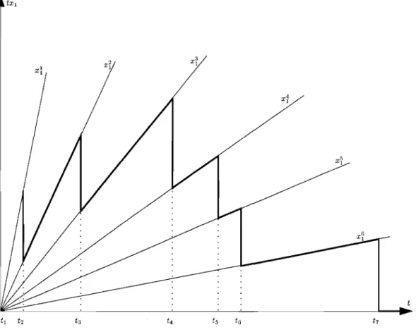
discontinuous at points t that induce a change of optimal basis in the lower level problem. We illustrate the evolution of the objective function tXI with respect to

the tax t in Figure 2.1, where

(xL

X₂₎ is the optimal solution of the lower level

problem corresponding to a tax

t

with values between

t

i _and

_t

i

+1.

Figure 2.1: Evolution of the objective function tXI with respect to tax t

An optimal pricing policy consists in setting

t

high enough to generate large revenues for the leader but, at the same time, low enough to promote the use of taxed activities corresponding to Xl by consumers.

The Network Pricing Problem is a particular case of a bilinearjbilinear pricing problem, which involves a transportation network and considers the arcs of the

network as activities. We present this problem in the next section.

2.3 The Network Pricing Problem

Let us define a transportation network as a set of nodes (cities) and a set of arcs (routes) linking sorne of these nodes together. At the upper and lower level, consider an authority and a set of network users respectively. We also define a commodity as a set of network users travelling from the same origin to the same destination.

In addition to a fixed cost associated with every arc, toUs are imposed by the authority on a specified subset of arcs of the network. Renee the Network Pricing Problem consists of devising toUlevels on the specified subset of toU arcs in order to maximize the authority's revenues. Then, reacting to the toUs, each commodity travels on the shortest path from its origin to its destination, with respect to a cost equal to the sum of toUs and initial costs.

Let us now introduee additional assumptions. First, in order to avoid trivial solutions leading to infinite revenues for the authority, we assume that there exists a toU free path for each commodity. Further, we restrict our study to non negative toU vectors.

Rowever, note that there exist models (see Labbé et al. (1998, [43]), Cirinei (2007, [16]) or Brotcorne et al. (2001, [12])) which also aUow negative toUs. The latter yield compensations with other (positive) toUs, when the corresponding arcs are used by multiple commodities. Even if such situations will not be considered in the thesis, the reader should know that there exist more realistic (but also more complex) models, which consider congestion effects (see for example Fortin (2005, [28])) and/or a non uniform distribution of the fixed cost perception in a population (see for example Marcotte et al. (2007, [51])).

The small network example depicted in Figure 2.2 illustrates the Network Pric-ing Problem. Assume that a commodity composed by a sPric-ingle user travels from node 1 to no de 5, the bolded arcs (2,3) and (4,5) being the toU arcs.

9

Figure 2.2: Network example

If we look closely at that network, we conclude that the user will never pay more that 22, which is the cost of the toll free path 1 ---> 3 ---> 5. In contrast, if the authority sets all tolls to zero, the user will choose the path 1 ---> 2 ---> 3 ---> 4 ---> 5 with cost 6. It means that an upper bound on the authority revenues is 22 - 6

=

16.

However, this bound is not always reached, as in the example. Whatever the tolls imposed by the manager, its revenue will never exceed 15. Indeed, the toll arc (2,3) can only be selected by the network user if the toll on this arc is less or equal to 5, because of the arc (2,4) ((2

+

x)

+

2

:S

9). In the same manner, the toll arc (4,5) can only be used if the corresponding toll does not exceed 10, because of the arc (3,5) (2

+

x

:S

12). An optimal solution for this example consists in setting tolls of 5 on the arc (2,3) and 10 on the arc (3,5).

The bilinear/bilinear bilevel Network Pricing Problem was first introduced by Labbé et al. (1998, [43]). Consider a multi-commodity network defined by anode set

N,

an arc set

A

u

B

and a set of origin-destination pairs

{(ok,

d

k) :

k

E

Je},

called commodities, each one endowed with a demand T/k. Let

A

be a subset of arcs a upon which tolls

ta

can be added to the original fixed cost vector c and B the complementary subset of toll free arcs, for which the cost vector c is also given. Assuming that, for a given toll policy t

=

(ta)aEA,

the network users travel

on short est paths with respect to the toUs and fixed costs on arcs, the Network Pricing Problem consists of devising a revenue maximizing toU policy. Upon the introduction of vectors

xk

=

(X~hEJC,aEA that specify the flows on commodities

k E K (i.e., x~ = 1 if commodity k travels on the toll arc a and x~ = 0 otherwize), the Network Pricing Problem can be formulated as the bilevel program (Labbé et al. (1998, [43])):

(TP)

subject to:

ta

2:

0 \faEA (2.1)

X

E

argm~n

L (L(Ca

+

ta)x~

+

L

cax~)

kEJC aEA

aEB

(2.2)

subject to: -1 if i = ok

L

x~+

L

x~-

L

x~-

L

x~=

1 if i = dk

aEi+nA

aEi+nB

o

otherwise \fk E K, \fi E

N

(2.3) x~ E

{O,

1} \fk E K, \fa E A, (2.4)

where i- (resp. i+) denotes the set of arcs having node i as its head (resp. tail). Note that the characterization of lower level solutions as origin-destination paths carrying either no flow or the total origin-destination flow aUows to obtain an integer programming formulation of (TP) that involves binary variables. Now, in view of the unimodularity of the constraint matrix associated with the shortest path problem at the lower level, one may drop the integrality requirements for the flow variables x. It foUows that the lower level problem can be replaced by its primaI dual constraints and primaI-dual optimality conditions, yielding a

single-level program involving complementarity (Le., disjunctive) constraints. Through the introduction of auxiliary variables

{

ta if commodity k uses arc a E A, k

Pa

a

otherwise

corresponding to the actual unit revenue associated with arc a E

A

and commodity k E K, Labbé et al. (1998, [43]) der ive a mixed integer linear formulation for this problem, namely (TP2) max

L L

rlp!

kEIC aEA subject 1.0:

Vk

E

K, Vi

EN (2.5)

>'~(a)

>.k

_{t(a) ::; Ca}

₊

_ta

_Vk

_{E K,}

_Va

_E

_A

_(2.6)

>.k

_{h(a) -}

>.k

_{t(a)::; Ca}

_Vk

_{E K,}

_Va

_E

_B

_(2.7)

L(

_CaXa

k

₊

Pa

k)

+

L

CaXa

k >.k

= d_k -

>.k

Ok

Vk

E K (2.8) aEA aEB

p! ::; M:x!

Vk

E

K, Va

E

A

(2.9) ta -

p! ::;

Na

{1

x~)

Vk

E

K, Va

E

A

(2.10)

p! ::;

ta

Vk

E

K, Va

E

A

(2.11)

p!

~ 0

Vk

E

K, Va

E

A

(2.12) x~ E

{a,

1}

Vk

E

K, Va

E

A

(2.13)

xk

_{a -}

>

0

Vk

E

K, Va

E 8, (2.14)

where h(a), t(a) correspond to the head and tail of the toU arc a E A, while M: and Na are sufficiently large constants.

Constraints (2.5) describe fiows on commodities. (2.6), (2.7) and (2.8) are the primal dual constraints and optimality conditions of the lower level problem. Con-straints (2.9), (2.10) and (2.11) come from the modellinearization, and ensure that p~

=

tax~ for aU k E K, a E

A.

Roch et al. (2005, [57]) and Grigoriev et al. (2005, [32]) prove the NP-hardness of this problem, even under restrictive conditions such as a single commodity or lower bounded toUs (see Labbé et al. (1998, [43])). However, several particular cases are polynomiaUy solvable, such as the Network Pricing Problem with a single toU arc (see Brotcorne et al. (2000, [11])). Van Hoesel et al. (2003, [65]) prove that, when the number of toU arcs is upper bounded, the optimal solution of the Network Pricing Problem can be obtained by solving a polynomial number of linear programs. The latter also present other particular polynomial cases of the problem.

In contrast with (TP2) formulation, in which the paths chosen by commodi-ties are described by fiows on arcs (latter caUed 'arc formulation'), Bouhtou et al. (2003, [7]) and Didi et al. (1999, [24]) propose formulations involving directly fiows on paths for commodities. Bouhtou et al. also propose a standard graph represen-tation of a network together with reduction methods for this last one, which often lead to a significant reduction of the network graph. This aUows obtaining good numerical results for medium size instances. Tests on randomly generated prob-lems involving 15 to 80 commodities and 20 to 100 toU arcs (in networks with 75 or 100 nodes and 2000 or 4000 arcs) show that an optimal solution can be identified within a couple of seconds. However, note that these instances lead to only 2 or 3 non dominated paths on average for each commodity, and thus are rather easy to solve.

Unfortunately, a commercial solver for linear programs such as Xpress cannot solve large size instances, neither of the (TP2) arc formulation presented ab ove nor of the path formulation. This is mainly due to the bad quality of the linear relax-ation in variables x (i.e., (2.13) are replaced by 0 :::; x~ :::; 1 for all k E /C, a E A). To overcome this problem, several approaches are considered.

Dewez et al. (2007, [23]) set values for constants M:, Na : k E /C, a E

A

of (TP2) formulation by computing upper bounds on the tolls on arcs, and propose valid inequalities for the various models (arc formulation and path formulation). Numerical tests have been carried out on randomly generated problems involving 20 to 40 commodities and 5% to 20% toll arcs, in networks with 60 nodes and 208 arcs, latter called 'grid graphs'. The results show that the adjustment of constants makes it possible to divide by two the value of the duality gap at the root of the branch and bound tree, whereas the valid cuts allow a reduction of the explored nodes as well as the computing time.

Cirinei (2007, [16]) proposes a column generation algorithm for the inverse op-timization problem, which consists of devising the tolls that should be imposed on the network, considering that the reaction of the network users is known and maximizing the authority's revenue. Tests on randomly generated problems involv-ing 10 to 40 commodities and 15% toll arcs in grid graphs show that the method performs well in terms of computing time. All instances can be solved in a couple of seconds. The column generation algorithm also allows to solve the largest in-stances much faster than without the algorithm. Further, the author proposes an exact resolution algorithm based on an intelligent enumeration of the solutions of the lower level problem. This resolution method allows to define improved upper bounds on the authority's revenue.

heuristic methods for the Network Pricing Problem. Brotcorne et al. (2001, [12]) present two heuristics for the problem: the first consists in setting toUs sequentiaUy over the arcs, while the second is based on a primaI-dual approach. Tests on prob-lems involving 10 to 20 commodities and 5% to 20% toll arcs in grid graphs show that heuristic solutions are on average within 1.5% and 7% of optimality respec-tively. Both heuristics are mu ch faster than an exact resolution. The latter (2000, [11]) also examine a very similar problem, in which commodities have to be routed from several locations to customers according to their respective demands.

AIso, Roch et al. (2005, [57]) propose an approximation algorithm for the single commodity Network Pricing Problem, with a guaranteed performance of ~ log n+ 1, where n is the number of toU arcs in the network.

FinaUy, Cirinei (2007, [16]) presents a tabu based local search algorithm, which exploits the underlying network structure of the lower level problem. This last method is very efficient, both in terms of solution quality and computing time, producing heuristic solutions within 1% of optimality for instances involving 10 to 100 commodities and 5% to 20% toU arcs in grid graphs.

Dewez (2004, [22]) also studies a particular case of the Network Pricing Prob-lem that deals with specific network structures similar to highways. lndeed, the model considered involves a path of toU arcs as weU as Triangle inequalities on the toU variables. She proves that, when it reduces to a single commodity, the prob-lem is polynomiaUy solvable. She presents an exact resolution algorithm for the multi-commodity problem, based on an enumeration of the solutions of the lower level problem. Unfortunately, due to the enumeration at the lower level, the time needed to solve the problem to optimality grows exponentiaUy with the number of commodities and the number of nodes in the network.

The author also proposes several heuristics to set the flow variables for this problem. Then the inverse problem aUows to determine the toUs yielding the best

20

revenue for the authority, once flows are fixed. We briefly describe the ide a behind the three best heuristics.

1) For each commodity k E K, set x~

=

1 for the toU arc a with the largest upper bound

M; :

a E A. Then solve the inverse optimization problem to find the toUs leading to a maximal revenue for the authority.

2) For each commodity k E K, set x~

=

1 for the toU arc a with the largest upper bound M; : a E A. Then observe that, if two commodities use the same toU arc a E A, the leader could take advantage to force the use of another toU arc

b

E

A \ {a}

(i.e., x~

=

1) for one of both commodities (with respect to the demand

T/

and the upper bounds M;). Next, solve the inverse optimization problem to find the toUs leading to a maximal revenue.

3) For each commodity k E K and for each toU arc a E A, set x~

=

0 if

M;

<

ex maxkEK

M;

(0

:s:

ex

:s:

1), i.e., if the upper bound on the revenue

M:

is too smaU with respect to the upper bound on the same arc a for other commodities. Then solve the remaining problem.

When tested on grid graph instances involving 21 to 36 commodities and 10 to 20 toU nodes in the highway, the best heuristics produce solutions within 5% of optimality in a couple of seconds.

Grigoriev et al. (2005, [32]) consider another particular case of the Network Pricing Problem, where each commodity chooses at most one toU arc from its ori-gin to its destination. As this specifie network structure looks like a town divided by a river with crossing bridges or tunnels, this problem is caUed the Cross River Network Pricing Problem. The authors prove that this particular problem is NP-hard.

tolls on the arcs are all equal, constitutes an O(n)-approximation algorithm (where n is the number of toll arcs in the network) for the Cross River Network Pricing Problem. Under sorne particular assumptions, the Uniform Network Pricing Prob-lem provides an O(log n)-approximation algorithm for the same probProb-lem.

We conclude this chapter with a summary (see Figure 2.3) of the main contri-butions to the Network Pricing Problem in literature.

J

Arc formulation • • 1 Exact solution approaches: Labbé 98, Cirinei 07, Dewez 07 1 Inexact solution approaches: Brotcome 01, Roch 05, Cirinei 07 Hililhway Network Pricing Problem Path formulation Exact solution approaches: Didi 99, Bouhtou 03, Dewez 07

Cross River Network Pricing Problem

NETWORK PRICING WITH CONNECTED TOLL ARCS

In this chapter, we present the specifie Network Pricing Problem addressed in the thesis. First modeUed as a bilinear/bilinear bilevel pricing problem, it is reformu-lated as a single level linear mixed integer model. Next, we propose a new linear mixed integer formulation for the problem, together with settings of constants and a preproeessing of the network. FinaUy, the complexity of this specifie Network Pricing Problem is studied.

3.1 Network Pricing Problems with Connected ToU Arcs

We now focus on a particular Network Pricing Problem dealing with structured networks in which aU toU arcs must be connected and constitute a path. As these structures can represent features specifie to a real highway topology and for the sake of clarity, we define a highway as the path of toU arcs in the network. The first variant of this problem, caUed Basic NPP, is directly derived from the classical Network Pricing Problem. Rowever, the toUs are additive in this network structure, while toUlevels are usuaUy determined with respect to given entry and exit points on the highway. Renee, a second variant is considered, that involves a complete toU subgraph, i.e., each toU arc represents a toU subpath between two entry and exit points. It is caUed General Complete ToU NPP. FinaUy, a third variant, caUed Constrained Complete ToU NPP, involves a complete toU subgraph together with specifie constraints that link toUs on several paths.

The first variant is directly derived from the Network Pricing Problem presented in Chapter 2. Let us define a commodity as a set of users with the same origin and destination nodes. A commodity can either take the short est toU free path from its origin to its destination, or foUow the highway, using shortest toU free paths to and from the highway. We assume that users who have left the highway are not aUowed to reenter, which implies that paths are uniquely determined by their respective entry and exit nodes.

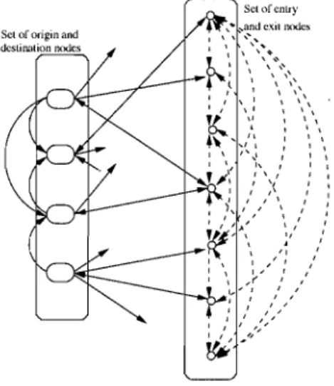
This problem is caUed the Basic Network Pricing Problem with Connected ToU Arcs, for short "Basic NPP". It is illustrated in Figure 3.1, where toU arcs are dashed. ToU free arcs are inserted between origin and destination nodes, as weU as from/to the origin and destination nodes to/from the highway. These arcs represent short est toU free paths between the corresponding nodes. We also assume that a fixed cost is set on each arc, and provides a measure of the distance, time or gas consumed on the arc. The fixed cost set on a toU free arc corresponds to the smallest fixed cost of a path between its nodes.

Set of ongin and destination nodes

Set of entry

and exit nodes

The mathematical formulation (TP2) presented in Chapter 2 applies to this situation. Rowever, additional constraints must be appended to (TP2) in order to ensure that a commodity which leaves the highway at sorne exit node does not reenter the highway at another entry node. Let us define the set

N

ç

N

of aIl possible origin and destination nodes, i.e.,

N

= {ok,dk :

k

E

K}.

Assuming that each shortest toU free path is represented by a single arc, the Basic NPP is described by model (TP2), with the additional constraints

L

x~+

L

x~

= 0 (3.1)

aEi+nB

Rowever, note that the toUs are additive in this network structure, i.e., a com-modity must pay the sum of the toUs on aU arcs that belong to its path. As toU levels are usuaUy determined with respect to given entry and exit points on the highway, we consider the Network Pricing Problem with Connected ToU Arcs in-volving a complete toU subgraph. Rence, as we assume that users who have left the highway are not aUowed to reenter, each toU subpath is represented by a single toU arc. This problem is depicted in Figure 3.2 and called "General Complete ToU NPP". Sel of cnLry , , , , , , , , ,

Let us now introduce sorne notation. For each arc a E A, let

t(

a), h( a) E

N

be its tail and head nodes respectively. For each commodity k E K and for each toU arc

a

E

A,

let c~ denote the fixed cost on the corresponding path Ok ---+

t( a)

---+

h( a) ---+ dk, where t( a), h( a) E

N

are the entry and exit nodes on the highway. The fixed cost on the toU free path Ok ---+ dk is denoted by C~d' while the corresponding fiow variable is X~d' For each commodity

k

E

K

and for each toU arc a E

A,

variable x~ represents the fiow on the corresponding path Ok ---+ t( a) ---+ h( a) ---+ dk, _while

variable ta is the toU on the arc a (i.e., toU subpath a). Further, we consider that

nodes are labeUed by the index 1 to m, leading to

lAI

=

n

=

m(m - 1) toll arcs. One obtains the foUowing bilevel formulation (2004, Dewez [22]):

(HP1) max

L L

rltax~

t,x kEK aEA subject to: ta :::: 0 'Va E A (3.2)

x

E arg mln

L (

Dc~

+

t")x~

+

c~x~)

(3.3) kEK aEA subject to:

LX~

+

X~d

=

1 'Vk E K (3.4) aEA x~ E

{O,

1} 'Vk E K, 'Va E A (3.5) X~d E

{O,

1} 'Vk E K (3.6)

Note that, as each toll subpath is now represented by a single toU arc, the fiow constraints (3.4) ensure that each commodity chooses either a toU path

a

(x~

=

1) or the toU free path (X~d = 1).

con-straint matrix associated with the lower level problem is unimodular. As a conse-quence, the lower level problem can be replaced by its primaI dual constraints and optimality conditions, yielding a single level program involving complementarity (i.e., disjunctive) constraints. Further, in order to obtain a linear model, variables

k {ta Pa

=

o

if commodity k uses arc a E A,

otherwise

are introduced, corresponding to the actual unit profit associated with arc a E A

and commodity k E K. This yields (2004, Dewez [22]):

(HP2)

maxLLr/p~

kEK. aEA subject to:

LX~

+

X~d =

1 Vk E K (3.7) aEA )..k

<

_- ck _a

+

t _a Vk E K, Va E A (3.8) )..k

<

_- ck _{od Vk} E K (3.9) L ( k k _caXa

₊

_Pa k)

₊

_codXod k k

₌

)..k _{Vk E K (3.10)} aEA p~ ~ M:x~ Vk E K, Va E A (3.11) ta - p~ ~ N a(l - x~) Vk E K,Va E A (3.12) p~ ~ ta Vk E K, Va E A (3.13) p~ ~ 0 Va EA (3.14) Xk _{ad -}

>

0 Vk E K (3.15) x~ E {O, 1} Va ~ A,Vk E K, (3.16)

where

M:

and Na are suitably large constants. For now, let us assume

M:

maXkEK.{c~d - c~} and Na

=

N

=

maXkEK.,aEA

M:.

Now, consider a network composed of three entry jexit nodes (labeUed 1,2,3) on the highway and two commodities kl , k2 E K with respective demands 7]kl

=

80,

7]k2

=

10. The fixed costs on paths c~ : k E K, a E A are described in Table 3.1,

while c~à

=

20 and c~â

=

21. The corresponding optimal toUs, according to model (HP2), are given in Figure 3.3.

ToU arc a ch a Ca k2 (1,2) 12 11 (1,3) 15 14 (2,1) 13 9 (2,3) 17 15 (3,1) 11 10 (3,2) 12 10

Table 3.1: Fixed costs c~ : k

=

kl , k2 , a E A for a network example with three entry jexit nodes on the highway

Q

JI \ \ I, \ \ I l \ \ 1 1 • \ l , 1 \ .: 8

0

'

,'10\ ~ 2 :9 1 1 1 1 1 4' 12' \ 1 \ 1 \ 1 1 1 \ 1 \ f \ 1 • 1

'~'

Figure 3.3: Optimal toUs

ta :

a E

A

for a network example with three entryjexit nodes on the highway

At optimality, commodity ki travels on the path Okl - 7 3 - 7 1 - 7 dk1 , while

commodity k2 travels on the path Ok2 - 7 2 - 7 1 - 7 dk2. One can observe that t2I = 10

<

t 3I = 9, i.e., the toU imposed on the path Ok2 - 7 2 - 7 1 - 7 dk2 is less

than the toU imposed on the path Ok2 --r 3 --r 1 --r dk2_{. While this can make sense} in the airline industry, where tickets correspond to specifie origin-destination pairs, this is unrealistic in a highway.

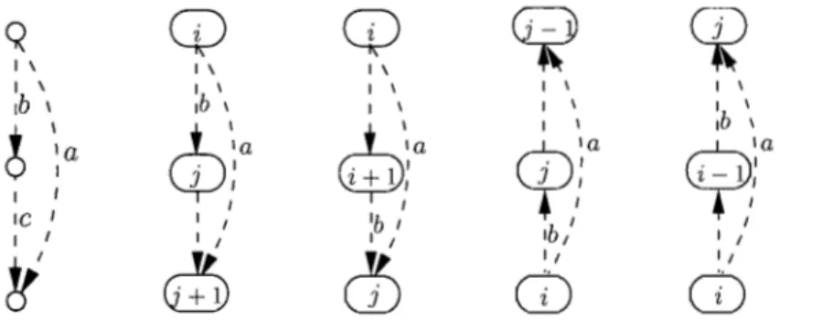
In order to prevent such situations, the Triangle and Monotonicity inequalities (3.17), (3.18) can be introduced, and the corresponding problem is called "Con-strained Complete Toll NPP".

Va,b,c E A: t(a)

=

t(b), h(b)

=

t(c), h(c)

=

h(a) (3.17)

Va,b E A:

t(a)

=

t(b)

<

h(a)

=

h(b)

+

1 or t(a)

=

t(b) - 1

<

h(a)

=

h(b)

or t(a)

=

t(b)

>

h(a)

=

h(b) - 1 or t(a)

=

t(b)

+

1

>

h(a)

=

h(b). (3.18) Triangle constraints ensure that between two given entry and exit nodes of the highway, a commodity would not take benefit from leaving the highway upstream and then reentering downstream latter. The Monotonicity constraints imply that the toU on a path cannot be less than the toll of any subpath. Subnetworks on which these inequalities apply are illustrated in Figure 3.4.

Q

CD

CD

~

~

1 \ 1 \ 1 \ 1 \ 1 \ 1 \ 1 \ 1 \ lb \ lb \ 1 \ 1 \ 1 \

t

\

cb\a

~\

1 \ lb \ la

la

cpla

9

1a

1 • 1 _{i +}

1:

• 1 i -

1':

] 1 ] 1 1 1 1 1 1 le 1 1

,

_{lb ,} Ib/

,

1

,

l , l , l ,

!f

@

_CD

l, l ,

cD

cD

Figure 3.4: Subnetworks on which Triangle and Monotonicity constraints apply

In the next section, we propose an alternative formulation for the problem. The latter does not involve dual variables and allows to express the optimality of the

lower level problem more explicitly in the constraints.

3.2 Model reformulation

While the lower level optimality conditions in (HP2) involve arc fiow variables, an alternative is to express the optimality of the lower level problem in terms of path fiows, without resorting to dual variables. The primaI dual constraints and optimality conditions (3.8), (3.9) and (3.10) of (HP2) are then replaced by the equivalent

Vk E K,Vb E A (3.19) aEA

Vk E K. (3.20) aEA

lndeed, these constraints ensure that the cost of the path chosen by commodity

k

E

K

at optimality is smaller than (or equal to) the cost of any other path for this commodity.

However, the second family of constraints (3.20) is obviously redundant due to constraints (3.7), (3.11) and the definition of constants M~ : k E K, a E A. Next, based on constraint (3.7), variables x~d can be removed, yielding the more compact

model: (HP3)

maxLLrlp~

kEK aEA subject to:

L

x~

:s:

1 Vk E K (3.21) aEA

L

(p~

+

c~x~)

+

c~d(l

-

L

x~)

:s:

ta

+

c~

Vk E K,Va E A (3.22) bEA bEA p~

:s:

M:x~ Vk E K,Va E A (3.23) ta - p~

:s:

Na(1 - x~) Vk E K,Va E A (3.24) p~

:s:

ta Vk E K, Va E A (3.25) p~

2.

0 Va E A (3.26) x~ E {O, 1} Vk E K,Va E A, (3.27)

In the sequel, we consider two variants of this program. In the General Com-plete ToU NPP (GCT-NPP), tolls are independent, while the Constrained Complete ToU NPP (CCT-NPP) imposes Triangle and Monotonicity con-straints (3.17) and (3.18). The corresponding models are labelled (HP3) and (HP3*) respectively.

Unfortunately, these models contain a large set of variables, especially for de-scribing flows on paths x~ :

k

E

K,

a E

A.

The next section provide suggestions to reduce the size of the problem, i.e., to set several flow variables to zero before solving the problem.

3.3 Preprocessing

Thanks to the complete toU subgraph structure, each feasible path from an ori-gin to a destination contains a single toU arc, and there exists a bijection between the toll arc set for a commodity and the corresponding path set. Further, the paths that are never used by a given commodity can be deleted, i.e., the corresponding flow variables are set to zero.

Property For each commodity k E K, the toll arcs a E A such that c~

>

c~d are never used, i.e., one can set x~ O.

For the Constrained Complete Toll NPP, an improved preprocessing can be applied according to the Monotonicity constraints. Let us introduce the following definition. An illustration of this definition is provided in Figure 3.5.

Definition 7 FoT' aU a in A, the following set is defined:

Ca

{b

E

A:

t(a) :::; t(b)

<

h(b) :::; h(a)

OT'

t(a)

~

t(b)

>

h(b)

~

h(a)}.

In the CCT-NPP, the toll variables must be such that

ta

~

tb

for all

b

in

~. According to the following proposition, for each commodity, several additional paths (toU arcs) are never used, and the corresponding flow variables can be set to zero.