HAL Id: hal-03196288
https://hal.insa-toulouse.fr/hal-03196288
Submitted on 12 Apr 2021HAL is a multi-disciplinary open access archive for the deposit and dissemination of sci-entific research documents, whether they are pub-lished or not. The documents may come from teaching and research institutions in France or abroad, or from public or private research centers.
L’archive ouverte pluridisciplinaire HAL, est destinée au dépôt et à la diffusion de documents scientifiques de niveau recherche, publiés ou non, émanant des établissements d’enseignement et de recherche français ou étrangers, des laboratoires publics ou privés.
Indoor thermal behaviour of an office equipped with a
ventilated slab: a numerical study
Matthieu Labat, Ion Hazyuk, Matthieu Cezard, Sylvie Lorente
To cite this version:
Matthieu Labat, Ion Hazyuk, Matthieu Cezard, Sylvie Lorente. Indoor thermal behaviour of an office equipped with a ventilated slab: a numerical study. Journal of Building Performance Simulation, Taylor & Francis, 2021, 14 (3), pp.227-246. �10.1080/19401493.2021.1905714�. �hal-03196288�
1
Indoor thermal behavior of an office equipped with a ventilated slab: a
numerical study
Matthieu Labat*1, Ion Hazyuk2, Matthieu Cezard1,3, Sylvie Lorente1,4
1LMDC, INSA/UPS Génie Civil, 135 Avenue de Rangueil, 31077 Toulouse cedex 04 France.
2Institut Clément Ader, Université de Toulouse, INSA/ISAE-SUPAERO/MINES-ALBI/UPS/CNRS,
31400 Toulouse, France
3IC Entreprises, Immeuble Le Volta – 17/19 rue Jeanne Braconnier - 92360 MEUDON LA FORET 4Villanova University, Department of Mechanical Engineering, Villanova, PA 19085, USA
*Corresponding author: m_labat@insa-toulouse.fr
Abstract
Ventilated slabs are used to provide indoor comfort by taking advantage of thermal inertia. The
underlying difficulty is that the computational cost is high, which is hardly compatible with an
exhaustive study of dynamic behavior at room scale. This paper presents a methodology for obtaining
a lumped model based on the identification of the transfer functions for constant airflow rate systems.
The transfer functions were combined into a state space model, which is able to obtain the main heat
fluxes with good accuracy at a much lower computational cost. The study moved to room scale in
order to further understand how a ventilated slab influences the heat balance. Increasing the number
of ducts promoted better indoor temperature stability but the impact was slight. The mass flow rate,
on the other hand, appeared to be crucial. This result underlines the need to tailor a control law
specifically to the ventilated slab.
Keywords:
TABS, ventilated slab, state space model, thermal inertia
2
Latin Symbols Description Unit
A Area m2
Cp Specific heat capacity J.kg-1.K-1
d Diameter m
f Frequency s-1
fD Darcy friction factor -
E Energy consumption J
F Transfer function
H Thickness of the slab m
h Convective heat transfer coefficient W.m-2.K-1
k Thermal conductivity W.m-1.K-1
K Static gain
L Length of the slab m
P Period s
pd Perimeter of the duct cross-section m
p Pole of a transfer function s
𝑄̇ Heat flux W
𝑚̇ Mass flow rate kg.s-1
Nu Nusselt number - Pr Prandtl number - Re Reynolds number - s Laplace variable - T Temperature K or °C t Time s
U Overall heat transfer coefficient W.m-2.K-1
V Volume m3
W Center-to-center duct distance m
z Zero of a transfer function
Greek Symbols α Thermal diffusivity m2.s-1 ρ Density kg.m-3 τ Time delay s Subscripts a air
3
c concrete
D ducts
f floor
in Inlet of the pipe
L Loads
S Stored
T Transmitted to the room
u Upper face W Wall Upper scripts ̅ Mean value ̂ Amplitude
1. Introduction
Thermally Activated Building System (TABS) are parts of building structures that are used to store
energy and release it later. This denomination refers notably – but not exclusively – to concrete floors
or ceilings with embedded water pipes, as exemplified in (Antonopoulos and Tzivanidis, 1997;
Koschenz and Dorer, 1999; Zhang et al., 2012). TABS have been attracting the interest of researchers
in recent decades (Romaní et al., 2016). The reason is to be found in the great thermal comfort they
can offer while saving energy, taking advantage of the use of radiative heat transfer (Rhee et al., 2017)
and high thermal inertia. While modern TABS often use water as the heat transfer fluid, mostly because
it has high density and specific heat, the concept of storing heat in a building structure is quite ancient
and initially used air as the medium to transport heat. It can be traced back thousands of years and has
been found in multiple locations across the globe. The huoqiang, which consisted of baked earth, is
believed to have matured and given birth to the Chinese kang (Bean et al., 2010). (Zhuang et al., 2009)
explain that, during the 1990’s, the Chinese government promoted the use of a more modern, more
efficient kang, which is elevated and thus uses both faces for heat transfer. The Korean ondol is a
4 buildings. Ancient Roman public bathhouses comprised several baths of different temperatures, heated
thanks to what we call a hypocaust. (Thébert, 2003) presents several archeological sites attesting to
the presence of heated public baths that prefigured the modern hypocausts. In (Basaran and Ilken,
1998), the energetic efficiency of such a system is debated. Later, in Europe, (Evelyn, 1691) described
a greenhouse heated by an outside furnace with pipes running underground along the whole length of
the greenhouse floor. Liverpool Cathedral used an air-based radiant heating system (Haden, 1924),
where the air flowed in a closed loop.
More recently, TABS using hollow-core concrete slabs can be found. These are elements produced in
factories before being assembled on site. The standard width of these hollow-core slab elements is
around 1.20 m (Corgnati and Kindinis, 2007; Mohammad et al., 2014; Russell and Surendran, 2001;
Winwood et al., 1994). At first, the cores were used to lessen the weight of the slab and to reduce
production costs. Their reduced self-weight enabled them to provide long spans. They also offered the
possibility of running electric cables or plumbing pipes within their cores. Soon, the cores began to be
used to circulate air and avoid using false ceilings. The best documented of these systems is the
TermoDeck® system. In a patent granted in 1971 for a “Method and device for controlling the
temperature in a premise”, a hollow-core slab using throttles inside the channels was presented. The throttles could rotate and directed air to different parts of the channel walls. In (Wachenfeldt and Bell,
2013), however, it is reported that the early versions of the TermoDeck® installed in the 1980s often
used under-sized ventilation, leading to discomfort.
Another kind of ventilated slabs are embedded-air-duct systems. Unlike hollow-core concrete slabs,
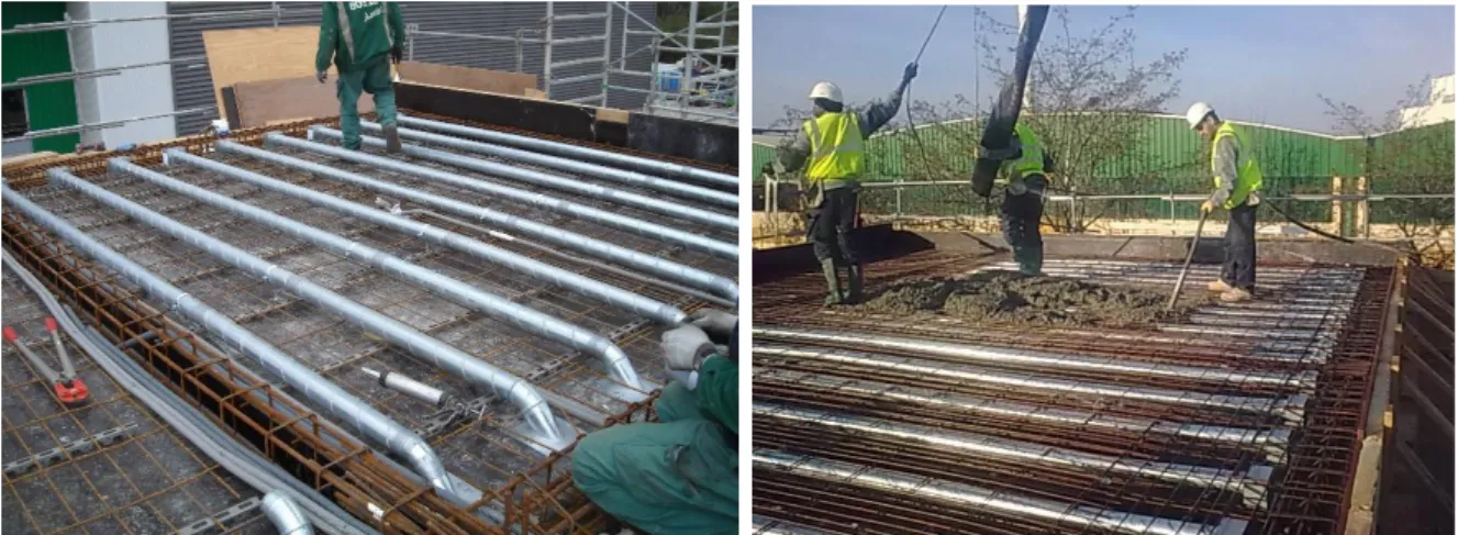
embedded-air-duct systems are cast in situ. Ducts are simply laid on the formwork and then concrete
is poured over them (see Figure 1). It is possible to vary the duct spacing, dimensions and shapes more
freely than when using hollow-core concrete slab. Using ventilated slabs also avoids the need for false
5 and, in turn, cost savings can be made. In real estate terms, this means that, for a given height, more
stories can be built when using this kind of system.
Figure 1: Photographs of the ventilation ducts before and during concrete pouring.
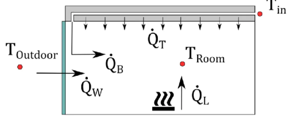
However, using air-based TABS impacts significantly heat transfer at the room scale compared to classical “all by air” systems. As illustrated in Figure 2, the outdoor air is prepared in a HVAC system prior to being blown through the slab. Part of the heat is transferred to the room by conduction through
the slab and then by convection and radiation, 𝑄̇𝑇, and another part is blown into the room 𝑄̇𝐵. For a
classical “all by air system”, the heat is provided by 𝑄̇𝐵 only. On the one hand, the calculation of 𝑄̇𝑇 is not straightforward because of the 3D nature of the heat transfer that takes place into the TABS.
Besides, the slab that surrounds the pipes brings a significant thermal inertia, stressing the need for
time-dependent model for estimating the heat transfer accurately. On the other hand, TABS system
allow exchanging heat over a large surface, which helps in providing comfortable indoor conditions.
6
Figure 2: Integration of the ventilated slab at the room scale
The coupling of air-based systems with the room is more pronounced than water based systems, since
the fluid is used for maintaining the indoor temperature within a comfortable range and for air renewal.
While the physics of heat transfer within the slab does not differ significantly, embedded-air-ducts are
facing other constraints than water based systems, which result in different designs. For example, the
mass flow rate has to meet minimal flowrate requirements for hygiene purposes, and to remove indoor
moisture. It is also limited in order to avoid undesirable effects that can occur at higher velocities (noise
and draught). As a consequence, the design and/or analysis of air-based systems differs from that for
water based systems.
Parametric studies of air-based TABS have already been proposed by other authors, giving some trends
that are briefly summarized below.
1. The influence of the airflow rate was discussed in (Isanska-Cwiek, 2005; Winwood et al.,
1997a, 1997b; Zmeureanu and Fazio, 1988). Logically, increasing the mass flow rate provides
more heat (or cold for a cooling application) to the room. But a less intuitive finding was that
increasing the mass flowrate reduced the fraction of the heating / cooling provided to the room
by conduction through the slab (𝑄̇𝑇 in the present study) and increased the fraction of the
heating / cooling provided to the room by direct air blowing (𝑄̇𝐵 in the present study).
2. The influence of the air path was discussed by (Barton et al., 2002; Winwood et al., 1997a) for
the TermoDeck® system. They showed that increasing the number of activated cores decreases
7 of heat being exchanged with the slab. The same conclusion was obtained by Park and Krarti
(2015), who found an asymptotic value for both heating and cooling modes.
3. Zmeureanu & Fazio (1988) varied the slab thickness from 10 to 20 cm, the cores being placed
in the middle of the slab. They found that this parameter was meaningful at low ventilation rate
but its influence diminished strongly as the airflow rate increased. A wider range of core depths
was tested at low velocities (Park and Krarti, 2015) and illustrated the non-negligible influence
of this parameter on the average heat transfer rate.
4. The high thermal inertia of concrete makes it interesting for TABS, yet this is offset by a rather
low thermal conductivity. Winwood et al. (1997a) compared two concrete slabs for which
thermal conductivity was increased by 10 and 20% by using aluminum seeding. Their results
show that this has little or no impact on the outlet temperature. Recently, another approach
based on the inclusion of Phase Change Materials (PCM) in mortars was proposed (Faheem et
al., 2016; Guo et al., 2020) to increase the performance of the system.
The underlying difficulty in studying embedded air duct systems is that the computational cost is high,
which is hardly compatible with an exhaustive study of their dynamic behavior. This has an adverse
effect when it is necessary to deal with the control of TABS, which is crucial (Gwerder et al., 2008;
Romaní et al., 2016). For this reason, many authors have used lumped parameter models, which are
able to reproduce the results obtained with detailed physics-based simulations with reasonable
accuracy but at a much lower computational cost. Some examples can be found in (Fonseca, 2011;
Gwerder et al., 2008; Weber and Jóhannesson, 2005) for water based systems. Fewer publications are
available for air-based systems, with the notable exceptions of (Chen et al., 2013; Ren and Wright,
1998) in the framework of a hollow core concrete slab.
Different techniques are available to develop lumped models and are detailed in (Romaní et al., 2016).
A widespread technique used in thermal engineering relies on the thermal-electrical analogy to define
8 various building elements, including TABS (Gwerder et al., 2008; Viot et al., 2018; Weber and
Jóhannesson, 2005). The RC circuit is generally set first, then the numerical values of its components
are identified. While some RC circuits are now well known for some building elements, there are few
results for ventilated slabs, except in a study (Ren and Wright, 1998) proposing a 4R2C model for a
ventilated slab having its two faces exposed to different rooms. An acceptable accuracy of 0.9°C was
obtained for the room temperature but higher discrepancies were observed during highly transient
periods. The resistances were estimated from the geometrical description of the system while the
thermal capacitances were adjusted to fit the experimental results.
A similar approach was proposed in the commercial software TRNSYS (TRANSSOLAR
Energietechnik, 2017). While an analytical expression for an equivalent thermal resistance can be
found, it is much harder to define equivalent thermal capacitances. This is one of the reason why
advanced techniques are used to obtain equivalent capacitances, either from experimental results or
from numerical simulations. However, these parameters are often case specific, hard to generalize, and
their value is not always given.
Another technique relies on the use of transfer functions that define the relationship between one input
and one output of the system by using mathematical transforms such as the Laplace transform. They
can later be combined in a state space model that gives a linear combination of multiple outputs with
multiple inputs. The advantage of this technique compared to the use of RC systems is that the
expression of the lumped model does not necessarily have to be defined a priori. Its drawback is that
it is not able to model nonlinear processes, such as in the case of variable mass flow rate. Some
examples can be found (Chae and Strand, 2013; Strand and Baumgartner, 2005) of conduction transfer
functions that were first developed for hydronic systems then modified to suit hollow core systems. A
similar technique, named the frequency response, was used in (Chen et al., 2013) and allowed the
thermal behavior of the system to be modeled in the frequency domain. However these approaches
9 solved separately and its temperature distribution in the direction of the flow is considered stationary.
Finally, other approaches are also available, such as a statistical model based on a significant amount
of experimental data (Ferkl and Jan Široký, 2010).
This paper aims to contribute to the understanding of the thermal behavior of embedded-air-duct
systems at room scale. Specifically, we develop a methodology that utilize transfer functions that
includes fluid dynamics, identify and validate the transfer functions using a detailed physical model,
show how these transfer functions can be used to study the thermal performance at room scale, and
draw conclusions regarding the influence of certain design parameters on this performance. The results
will be set against the case of a conventional (non-ventilated) slab to highlight the benefits and the
drawbacks of the ventilated slab, as well as the impact of the number and size of the ducts.
The paper is divided in three parts. The first part (section 2) presents the detailed finite element model
of the ventilated slab. This detailed model will replace the real system for the next steps of the study.
The second part (section 3) presents the method used to obtain the lumped parameters model of the
ventilated slab out of the simulation data obtained with the detailed model. Finally the third part
(section 4) integrates the lumped parameters model of the slab at the room level and studies the impact
of the number of ducts and the flowrate on the thermal behavior of the room.
2. Physically based model of the ventilated slab
The objective of the physically based model is to generate data for the identification of the lumped
model and its validation. It relies on a finite element commercial software (COMSOL) to solve heat
transfer at the scale of the ventilated slab, while the heat transfers in the room and the HVAC system
are ignored for now.
The description of the ventilated slab proposed here was inspired by a full scale commercial prototype
10 GreenFloor® system prior to its commercialization. It was not intended to validate a heat transfer
model however, and many elements necessary for this purpose are lacking (insufficient number of
temperature and air flow measurements, unknown thermal properties for the concrete cast on site,
uninsulated sidings and/or thermal bridges). Furthermore, some buildings equipped with the
GreenFloor® system are already occupied. While they provide valuable information regarding the
operation of the system, they are not fully instrumented and cannot be used for validation purposes.
The slab is 5 m long (L) and 0.22 m high (H), and the diameter of the embedded ducts d is 0.08 m. The
ducts are placed regularly within the slab, their axes being spaced at W = 0.45 m apart. The system
should be considered as a juxtaposition of some elementary parts, as highlighted in light grey in Figure
3. This design was selected to fit the requirements for classical offices and can be extended to a larger
surface simply by adding elementary parts. In practice, the ducts are placed first and the concrete is
poured over the whole surface at once, so that there is no physical separation between the different
parts. The prototype and the system modeled here is a 20.25 m2 slab that involves 9 ducts. Therefore,
it can be broken down in 9 elementary parts.
Figure 3: Ventilated slab dimensions and identification of an elementary part of the slab
Since the pipes are regularly spaced, there is no need to model the whole slab, provided that there is
no heat transfer at the sides (the so-called thermal bridges). It is acknowledged, however, that the latter
might be sizeable, as underlined by (Park and Krarti, 2015). Here, the modelling of the slab will focus
11 Two different domains have to be considered here: the heat transfer within the slab and heat transfers
within the duct. For the slab, the classical heat equation in solids has to be solved.
𝜌𝑐𝐶𝑝,𝑐(
𝜕𝑇
𝜕𝑡) + 𝜵(−𝑘𝑐𝜵𝑇) = 0
(1)
The slab is homogeneous and made only of concrete. Classical thermal properties for concrete are
considered: a density of ρc = 2300 kg.m-3, a specific heat capacity of Cp,c = 880 J.kg-1.K-1, and a
thermal conductivity of kc = 2.2 W.m-1.K-1.
For heat and mass transfer within the duct, a comprehensive approach would require solving the mass
and momentum balances together with the heat balance. However, it would significantly burden the
model for uncertain improvements in terms of accuracy. Here, we observe that the nature of heat
transfer is not very different from those taking place in Earth to Air Heat Exchangers (EAHE). We
propose to use the approach presented in (Estrada et al., 2018), where heat transfers in only one
dimension are considered within the duct, while the pressure and velocity fields are not computed. For
a single element defined by its length dx and its cross-section A, the heat balance yields:
𝜌𝑎 𝐴 𝑑𝑇 𝑑𝑡 = −𝑚̇𝑎 𝑑𝑇 𝑑𝑥+ ℎ𝑐 𝑝𝑑 𝐶𝑝,𝑎 (𝑇𝑤− 𝑇) (2)
The air thermal properties are assumed constant and set to ρa = 1.2 kg.m-3 for the density and
Cp,ca = 1003 J.kg-1.K-1 for the specific heat capacity. The value for the convective heat transfer coefficient hc is set as shown in Eqs. (3) to (5) (Holman, 1986).
ℎ𝑐 =𝑘𝑎 𝑁𝑢𝑑 𝑑 (3) 𝑁𝑢𝑑 = (𝑓8 )𝐷 (𝑅𝑒𝑑 − 103)𝑃𝑟 1 + 12.7 (𝑓8 )𝐷 1 2 (𝑃𝑟23− 1) (4) 𝑓𝐷 = (0.79 𝑙𝑛(𝑅𝑒𝑑) − 1.64)−2 (5)
12 where ka is the thermal conductivity of air, set at 0.025 W.m-1.K-1.
The coupling between the slab and the duct is made through the wall temperature Tw, averaged over
the perimeter of the duct cross-section for every position along its axis. In return, the convective heat
flux computed within the pipe is used as a boundary condition for the slab.
As mentioned earlier, one of the strengths of the ventilated slab is to remove the need for false ceilings,
providing more compact office buildings. However, it is unlikely that the rooms of two stories located
one above the other will have the same demand at the same time, simply because, for example, the
temperature set points might be different. Therefore, a ventilated slab cannot be used as a floor and a
ceiling air-conditioning system simultaneously. As the cooling demand is significantly higher than the
heating demand in modern offices, the ventilated slab should be used as a cooling ceiling in order to
take advantage of natural convection. Consequently, the boundary conditions are the following:
1. The air temperature at the inlet of the duct Tin is fixed ;
2. There is no heat flux at the upper and side boundaries of the slab ;
3. A Robin boundary condition is applied to the lower part of the slab, namely by setting the
temperature of the room, TRoom, and a heat transfer coefficient that accounts for both convective
and radiative heat transfer. This coefficient is set to 8 W.m-2.K-1.
A constant mass flow rate is used in this study. While it is acknowledged that variable air flow systems
are now widespread, it was anticipated that this technique would not suit the purpose of this study very
well. To a certain extent, varying the airflow rate would result in bypassing the thermal inertia of the
system and addressing indoor comfort mostly by the air blown into the room. Another reason for
considering a constant airflow rate is that it facilitates the identification of the lumped model. In this
study, we propose to use a 300 m3.h-1 airflow rate, which leads to an air renewal of approximately 6
ach. This value is higher than the requirement of the French regulations (1 ach in this case). However,
13 comfortable indoor conditions in most situations. Nevertheless, the influence of the airflow rate will
be illustrated later by repeating the computational work for 100 and 500 m3.h-1.
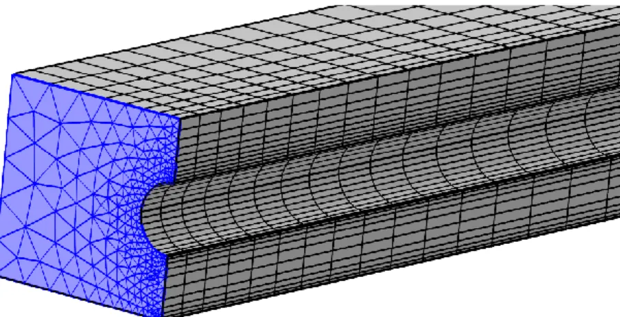
The problem was solved by using commercial finite element software (COMSOL). The meshing of
the slab was refined close to the pipe and to the lower surface. It was defined on the side at the inlet of
the pipe (450 surface elements), then swept along the pipe direction by using a distribution containing
50 elements, the size of which increased progressively toward this direction as shown in Figure 4. A
mesh distribution of 100 elements was used for the duct in 1D. The final mesh contained 22500
elements for the slab. Mesh sensitivity was tested by doubling the number of elements, which resulted
in only 1% difference in the air temperature at the outlet of the duct or in the heat flux at the bottom
of the slab. Finally, the problem was found to be sensitive to the time-step tolerance, which was set to
10-3.
Figure 4: Meshing of the slab surface at the inlet of the pipe (highlighted in blue) and swept mesh in the direction of the pipe axis.
In order not to stick to a single configuration of the ventilated slab, other geometries were tested by
changing the number of ducts (ND). To ease comparison, three constraints were imposed. Both the total
mass flow rate and the volume occupied by the ducts within the slab remained the same. Also, the
height (H) and length (L) of the slab remained constant for all cases. In consequence, the air velocity
14 briefly summarized in Table 1. Finally, the air flow rate was modified only for the geometry used as a
reference case, leading to a total of seven different systems.
Table 1: Parameters used for all the ventilated slabs
ND 3 6 9* 12 15 9 9 d (10-3 m) 139 98 80 69 62 80 80 W (10-2 m) 135 68 45 34 27 45 45 𝑚̇𝑎(kg.s-1) per duct 3.33 10 -2 1.66 10-2 1.11 10-2 8.33 10-3 6.66 10-3 5.53 10-3 1.85 10-2 ℎ𝑐 (W.m-2.k-1) 7.8 8.4 8.8 9.0 9.2 3.2 13.1 * Reference case
The methodology presented in this paper was set and validated for the reference case first, then applied
to all other cases.
3. Lumped model of the ventilated slabs
In this section, the input and the output of the transfer functions will be defined first, then the
identification methodology will be described. The behavior of the seven different systems will be
compared by means of Bode magnitude plots. Finally, the accuracy of the lumped (state space) model
will be discussed.
3.1. Definition of the inputs and outputs
A transfer function gives the relationship between an input and one output of the system. When the
system has several inputs and outputs, the number of transfer functions is equal to the product of the
number of inputs and the number of outputs. The first step consists in defining the inputs of the
ventilated slab and proposing relevant outputs. Our objective is to obtain a lumped model that is
suitable for computing the heat balance at the room scale, which, at steady state, is:
15 Here, Q̇𝐿 is the total of the heat loads of the room. It can be broken down into several terms to represent
the heat flux through the envelope and the ones resulting from the use of appliances for example.
However, it has an impact on the indoor temperature, TRoom, rather than on the ventilated slab itself.
For this reason, it will not be included in the definition of the transfer functions.
𝑄̇𝐻𝑉𝐴𝐶 is the heat flux provided to the room by an HVAC system by means of a ventilated slab.
Assuming that the pressure of the room is higher than outdoors and in the corridor, the mass flow rate
blowing into and out of the room are the same, so Q̇𝐻𝑉𝐴𝐶 can be defined by:
𝑄̇𝐻𝑉𝐴𝐶 = 𝑚̇ 𝐶𝑎 𝑝,𝑎𝑇𝑖𝑛− 𝑚̇ 𝐶𝑎 𝑝,𝑎𝑇𝑅𝑜𝑜𝑚 (7)
Now, considering that the ventilated slab is a subsystem of the room, this heat flux can also be broken
down into three terms as follows:
𝑄̇𝐻𝑉𝐴𝐶 = 𝑄̇𝑇+ 𝑄̇𝐵+ 𝑄̇𝑆 (8)
where Q̇𝑇 is the heat flux transmitted to the room by conduction through the slab, Q̇𝑆 is the heat flux
stored within the slab (null at steady state) and Q̇𝐵 is the heat flux blown into the room, given by:
𝑄̇𝐵 = 𝑚𝑎̇ 𝐶𝑝,𝑎(𝑇𝐵− 𝑇𝑅𝑜𝑜𝑚) (9)
From the slab’s perspective, it appears that the room temperature, Troom, and the inlet temperature, Tin,
are the only two exogenous inputs. The heat flux stored in the slab is not useful for computing the heat
balance at the room scale, so Q̇𝑇 and Q̇𝐵 were chosen as the two outputs. As a result, four transfer
functions have to be identified for the lumped model. A dimensionless form is preferred, giving:
𝐹𝑇,𝑇𝑖𝑛 = Q̇𝑇 𝑚𝑎̇ 𝐶𝑝,𝑎𝑇𝑖𝑛 𝐹𝑇,𝑇𝑅𝑜𝑜𝑚 = Q̇𝑇 −𝑚𝑎̇ 𝐶𝑝,𝑎𝑇𝑅𝑜𝑜𝑚 (10) 𝐹𝐵,𝑇𝑖𝑛 = Q̇𝐵 𝑚𝑎̇ 𝐶𝑝,𝑎𝑇𝑖𝑛 𝐹𝐵,𝑇𝑅𝑜𝑜𝑚 = Q̇𝐵 −𝑚̇ 𝐶𝑎 𝑝,𝑎𝑇𝑅𝑜𝑜𝑚
16 One of the drawbacks of the transfer functions in the case of multi-input/multi-output systems is that
the functions have to be combined linearly to compute the outputs. The definition proposed in (10)
enables us to write:
Q̇𝑇 = 𝑚𝑎̇ 𝐶𝑝,𝑎(𝐹𝑇,𝑇𝑖𝑛𝑇𝑖𝑛− 𝐹𝑇,𝑇𝑅𝑜𝑜𝑚𝑇𝑅𝑜𝑜𝑚)
(11) Q̇𝐵 = 𝑚̇ 𝐶𝑎 𝑝,𝑎(𝐹𝐵,𝑇𝑖𝑛𝑇𝑖𝑛− 𝐹𝐵,𝑇𝑅𝑜𝑜𝑚𝑇𝑅𝑜𝑜𝑚)
This will be finally achieved later, by transforming the transfer functions into a state-space
representation.
Next, a general expression of a transfer function can be given as follows:
𝐹(𝑠) = 𝐾 ∏ (𝑧1 𝑖𝑠 + 1) ∏ (𝑝1 𝑗𝑠 + 1) 𝑒−𝜏0𝑠 (12)
where s is the Laplace variable, K is the static gain, zi are the zeros, pj are the poles and τ0 is the time
delay. The objective is to propose a model with minimum coefficients and good accuracy.
Some constraints on the above parameters can be deduced from the physics of heat transfer. The static
gain of the transfer function is the ratio of one output to one input at steady state. Here, the static gain
for 𝐹𝑇,𝑇𝑖𝑛 and 𝐹𝐵,𝑇𝑖𝑛 represents the fraction of the heat flux provided to the slab that is transmitted or
blown to the room, respectively. At steady state, there is no heat flux stored within the slab, which
leads to:
𝐾𝐹
𝑇,𝑇𝑖𝑛 + 𝐾𝐹𝐵,𝑇𝑖𝑛 = 1 (13)
The same holds when the room temperature varies, and:
𝐾𝐹
𝑇,𝑇𝑖𝑛 = 𝐾𝐹𝑇,𝑇𝑅𝑜𝑜𝑚
𝐾𝐹
𝐵,𝑇𝑖𝑛 = 𝐾𝐹𝐵,𝑇𝑅𝑜𝑜𝑚
17 In the frequency domain, the transfer function can also be analyzed as the ratio of the output to the
input amplitudes depending on the frequency (f), the latter being included in the definition of the
Laplace variable. For rapid periodic variations of room temperature, the heat flux is adsorbed and
released by a thin layer of concrete in contact with the room air, having no impact on the wall
temperature, Tw, in the duct. In this case, the amplitude of the air temperature at the outlet of the duct
(denoted 𝑇̂) is null, leading to: 𝐵
lim
𝑓→∞𝐹𝐵,𝑇𝑅𝑜𝑜𝑚 = 1 −
𝑇𝐵 ̂
𝑇̂𝑅𝑜𝑜𝑚 = 1 (15)
The same thing happens when the inlet temperature Tin follows rapid periodic variations. The temperature in the vicinity of the duct varies but the temperature at the surface of the ceiling remains
constant, leading to:
lim
𝑓→∞𝐹𝑇,𝑇𝐼𝑛 = 0 (16)
3.2. Identification of the transfer functions
Early tests, not presented here, were achieved by using harmonic excitations of the inputs in order to
estimate the Bode diagram of the four transfer functions. This indicated that three transfer functions
would be correctly modeled by using 2 zeros and 2 poles. The Bode diagram was noticeably different
for FT,Tin, which should be modeled with only 1 zero and 2 poles. Finally, a 2.7 s delay (τ0) was identified for the transfer functions used to model the heat flux blown to the room (FB,Tin and FB,Troom).
Physically, this corresponds to the time taken by the air to move through the length of the pipe.
However, this time delay is very much lower than the other time constants, including the ones used for
control in buildings. It was therefore ignored.
Identification of the coefficients relied on the use of dedicated Matlab functions. Based on the least
squares method, it retrieves the coefficients that fit the time series used as a reference, which was
18 a constant time step for the whole time series. The frequency range that has to be explored thus gives
the minimum number of points of the time series (Nmin) as follows:
Δ𝑡𝑚𝑎𝑥 = 1 2 𝑓𝑚𝑎𝑥 𝑡𝑚𝑖𝑛 = 1 𝑓𝑚𝑖𝑛 𝑁𝑚𝑖𝑛 = 𝑡𝑚𝑖𝑛 Δ𝑡𝑚𝑎𝑥 = 2𝑓𝑚𝑎𝑥 𝑓𝑚𝑖𝑛 (17)
Here, Δ𝑡𝑚𝑎𝑥 is the simulation time step (which should satisfy the Shannon frequency) and 𝑡𝑚𝑖𝑛 is the
simulation time (which should represent at least one period of the smallest frequency). Early tests
showed that the frequency range of typical excitations of the system under study, and thus to be used
to plot the Bode diagram, was [10-8: 10-2] Hz, leading to the need to generate at least 2 106 points. As
this far exceeds the capacities of the software (limited to approximately 4 104 points, not to mention
the computational time), it was decided to split the identification process in two steps. First, the inputs
were generated in the low frequency range ([10-8: 10-5] Hz) by using a chirp signal, providing a signal
with a frequency that increased smoothly against time. Next, a Pseudo Random Binary Sequence
(PRBS) was used to explore the high frequency range ([10-6: 10-2] Hz). As it produces step-like
variations of the input, it covers a wider range of frequencies and imitates sudden temperature
variations that are likely to happen in reality, when a device is turned on for example. Thus, for the
first frequency range, we needed only 𝑁𝑚𝑖𝑛 = 2 103 points and, for the second one, 𝑁𝑚𝑖𝑛 = 2 104
points.
The reference values for the outputs were obtained by simulating the system in COMSOL with the
above input profiles. Based on this response, the identification can be broken down into three steps.
19 1. A steady state simulation was run first to identify the value of the static gain, which was
adjusted to fit (13).
2. The time series at low frequency was then used next to identify the poles and zeros situated
roughly in this frequency range, the static gain being fixed. Each transfer function had one pole
and one zero in this range.
3. The time series at high frequency was used next to identify the other poles and zeros (if any)
in order to improve the response fidelity, the other parameters being fixed. Here again, each
transfer function had one additional pole and one additional zero, except for 𝐹𝑇,𝑇𝑖𝑛 , which had
one additional pole only. They were slightly adjusted afterwards to meet the requirements of
(15).
The final expression for FB,Troom is given in (18) as an example.
𝐹𝐵,𝑇𝑅𝑜𝑜𝑚(𝑝) = 0.607 (7.46 10
4 𝑠 + 1)(1.16 104 𝑠 + 1)
(4.72 104 𝑠 + 1)(1.11 104 𝑠 + 1) (18)
Note that the second pole and zero are very close to each other. The improvement of the transfer
function obtained by adding these two coefficients is, in fact, negligible, and this equation could be
reduced. However, as these coefficients bring a physical meaning at high frequencies and as they do
not significantly burden the model, they were kept for this transfer function. The identification of
𝐹𝑇,𝑇𝑅𝑜𝑜𝑚 and 𝐹𝐵,𝑇𝑖𝑛 led to similar conclusions. The high frequency poles/zeros identified were,
however, outside the bandwidth of the excitation signals and were therefore removed. The values of
the coefficients for all the transfer functions are summarized in Table 4, which has been placed in the
appendix for the sake of clarity.
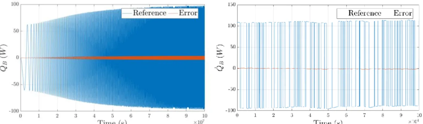
The output responses obtained with the physical model, which stands as the reference here, are
compared with those obtained with the transfer function FB,Tin in Figure 5 for illustration purposes. The
magnitude of the error lies roughly within the range of ± 4%. The model accuracy will be discussed in
20
Figure 5: Heat flux, QB, blown into the room when TRoom varies and error obtained with the
transfer function. Results obtained with a chirp signal can be seen on the left and a PRBS signal on the right.
3.3. Influence of the number of ducts
The methodology presented in the previous section was applied to the other four configurations of the
system, leading to a total of 20 transfer functions. They are compared by means of the Bode magnitude
plots presented in Figure 6 and Figure 7. For the sake of clarity, the Bode phase plots are not presented.
Figure 6: Bode magnitude plot for FT,Tin (left) and FT,TRoom (right) when the number of ducts, ND,
21
Figure 7: Bode magnitude plot for FB,Tin (left) and FB,TRoom (right) when the number of ducts, ND,
varies.
First of all, it appears that the magnitude remains constant for frequencies outside the [10-6: 10-3] Hz
range, with the notable exception of FT,Tin. The static gain corresponds to the magnitude obtained at
low frequencies and is discussed below. For three ducts (ND = 3), a larger fraction of the heat provided by the HVAC system is blown into the room (76%) than transmitted through the slab (24%) in the
steady state. Under the constraint of a constant volume occupied by the ducts, increasing the number
of ducts results in a more balanced distribution of the heat fluxes (54% and 46% respectively for fifteen
ducts).
Second, the shape of the Bode magnitude plot is approximately the same for FB,TRoom and FT,TRoom, i.e.
for the transfer functions related to the room temperature. The influence of ND at low frequencies was
already debated when discussing the static gain but it is noteworthy that it has no influence at high
frequencies. Therefore, discussion of the influence of ND can be based on the static gain and the transfer
functions related to the inlet temperature Tin only.
Next, the Bode magnitude plot for FT,Tin is similar to a low pass filter. Its cutoff frequency is
approximately 2.10-5 Hz, this value being only slightly dependent on ND (± 7% compared to the
reference case). In other words, the time constant of this filter is approximately 2.2 h. Moreover, at
high frequencies, the gain is roughly identical for all 𝑁𝐷. The heat flux transmitted through the slab
will not be significantly modified for rapid variations (shorter than 2.6 minutes) of the inlet temperature
Tin, because of its thermal inertia. On the other hand, a constant heat flux would be obtained roughly 6.6 h after a step variation of Tin (under the assumption of a constant room temperature).
Considering FB,Tin, the system behaves differently. Rapid variations of the inlet temperature, Tin, will
be passed on to the heat flux blown into the room, but with a smaller amplitude than for lower
frequencies, because of the heat transfer with the slab. Comparing this Bode plot with the one obtained
22 influence starts at roughly 7.10-6 Hz, and increases progressively with the frequency, up to an
asymptotic value that is reached for frequencies higher than approximately 5.10-4 Hz. Note that the
influence of ND is considerable here, as increasing the number of ducts will increase Q̇𝑆. For
fluctuations with periods lower than half an hour, the ratio of the amplitude of TB to the amplitude of
Tin is 66% for ND = 3, but drops to 30% for ND = 15. This means that 34% (70% for ND = 15) of the variation of the heat flux provided at the inlet is stored and released successively, smoothing the
temperature variation of the air blown into the room.
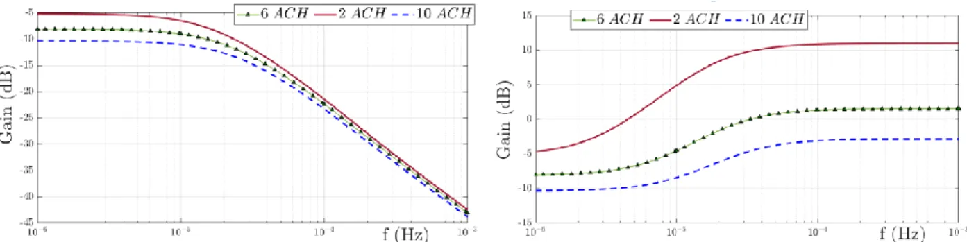
3.4. Influence of the mass flow rate at the scale of the ventilated slab
The influence of the mass flow rate was tested only for the ventilated slab equipped with nine ducts.
The mass flow rate was changed to 100 and 500 m3.h-1, values that are representative of an air renewal
of 2 and 10 ACH for the room located below the ventilated slab. The Bode magnitude plots of the
transfer functions are presented in Figure 8 and Figure 9. The values of the coefficients are given in
Table 5 in the appendix.
23
Figure 9: Bode magnitude plot for FB,Tin (left) and FB,TRoom (right) for different air change rates.
First, it can be observed that the time constants tend to increase when the airflow rate is lowered, and
conversely. This means that the system behaves more slowly for a lower air change rate, which is
equivalent to a system that provides more inertia. Considering the transfer functions related to the input
temperature Tin, the time constants vary slightly over the range [-35 : 35]%. The variation is more
pronounced for the transfer functions related to the room temperature (up to ([-170 : 75]% for FT,TRoom).
Second, the influence of the mass flow rate on the static gain is the most obvious. Reducing the mass
flow rate increases the fraction of the heat flux transmitted through the slab and diminishes the fraction
blown into the room, so that they reach 55% and 45%, respectively, for 2 ACH. The opposite happens
when the mass flow rate increases to 10 ACH, leading to 70% of the heat flux being blown into the
room at steady state. However, increasing the mass flow rate also means that the cooling power
provided to the ventilated slab is more important. It is interesting to observe that, despite a lower
fraction being transmitted to the room by conduction, the net heat flux would be the highest for 10
ACH under the assumption of steady state. This is summarized in Table 2, where the numerical values
have been calculated assuming a temperature difference of 12°C between the inlet and the room.
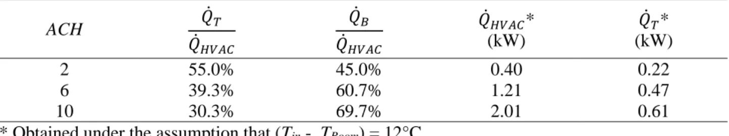
Table 2: Comparison of the heat flux obtained at steady state for different air flow rates.
ACH 𝑄̇𝑇 𝑄̇𝐻𝑉𝐴𝐶 𝑄̇𝐵 𝑄̇𝐻𝑉𝐴𝐶 𝑄̇𝐻𝑉𝐴𝐶* (kW) 𝑄̇𝑇* (kW) 2 55.0% 45.0% 0.40 0.22 6 39.3% 60.7% 1.21 0.47 10 30.3% 69.7% 2.01 0.61
* Obtained under the assumption that (Tin - TRoom) = 12°C
The sizing of most “all-by-air” systems for cooling relies on the limit imposed on the temperature
difference between the air blown into the room and the room itself. For the occupants’ comfort, this
difference should not be greater than 12°C. Then, the air flow rate is determined so that the system is
able to cope with the internal heat loads. Using a ventilated slab brings an alternative, as the
24 slab, Tin. In other words, the HVAC system could provide a lower airflow rate at a lower temperature.
However, this technique has to face two major drawbacks: first, the temperature of the surface of the
ceiling has to remain higher than the indoor dew point temperature. Second, this logic assumes a steady
state, so 𝑄̇𝑆 is zero. Given the time constants of the system, however, it is likely that the steady state
will hardly be reached in practice, stressing the need for dynamic simulations. These will be obtained
through the use of a state space model in this paper.
3.5. State space model and its validation
The four transfer functions can be combined in a state space model as follows:
{𝑦 = 𝐶𝑥 + 𝐷𝑢𝑥̇ = 𝐴𝑥 + 𝐵𝑢 (19)
where u and y are column vectors containing the inputs and the outputs, respectively, of the transfer
functions.
𝑢 = [𝑚̇𝐶𝑝,𝑎𝑇𝑖𝑛(𝑡) −𝑚̇𝐶𝑝,𝑎𝑇𝑅𝑜𝑜𝑚(𝑡)]𝑇
(20) 𝑦 = [Q̇𝑇(𝑡) Q̇𝑆(𝑡)]𝑇
x is a column vector containing the state variables. A, B, C and D are matrices that contain the parameters of the system. They can be related to the coefficients of the transfer function by using a
partial fraction decomposition. As this would not add value to this study, it will not be detailed here
and the values of the coefficients in the four matrices are not presented.
The sizes of these matrices depend directly on the number of poles of the transfer functions (for matrix
A), as well as the number of inputs (for matrix B) and the number of outputs (for matrix C). The
dimension of the state space model proposed here is 6. To validate the identified state space model, a
new simulation was run with the physically based model (Comsol model) but with an excitation
different from the one used for identification. The idea of doing this was to test the robustness of the
25 month at mid-season in an occupied building (see Figure 10), as they provide realistic temperature
ranges and variations. On the real TABS, the control was achieved by varying the air flowrate and
using a simple on/off control for heating or cooling. As a consequence, the inlet temperature (𝑇𝑖𝑛)
variations were rapid and in large magnitude. In the system studied in the present paper, temperature
variations at the inlet are expected to be smoother because of the use of a constant flowrate.
Nevertheless, using the in situ measurements will result in a validation test that is more demanding.
Conversely, the room temperature remained within a narrow range.
Figure 10: Inputs used to validate the state space model.
The results are compared in Figure 11 for the reference case (ND = 9), where positive values are used
when heating is provided to the room and negative values for cooling. Here, it should be recalled that
the transfer functions and the state space model were developed for an elementary part of the slab
containing only one duct. The heat fluxes have to be multiplied by 9 to be representative of a 20.25 m2
office, leading to an air-conditioning power magnitude of approximately ± 1.5 kW.
The mean error obtained with the state space model is lower than 0.03 W and 95% of the error remains
within a ± 2 W and ± 4 W interval, for the transmitted and blown heat fluxes respectively. This
represents a relative error of ± 10% with respect to the average heat flux in both cases. Overall, it
26 punctually when quick variations happen. They result from a small lag and do not lead to a significant
bias. This validation test was repeated for the other ventilated slab models and led to similar
conclusions.
Figure 11: Comparison of the results obtained with the physical and the lumped models for
ND = 9. Heat flux transmitted to the room through the slab (left) and blown into the room (right).
Finally, let us mention that the computational time required to run the validation test with the physical
model exceeded 17 h on a machine equipped with eight 2.2 GHz processors and with 100 Go RAM.
The results were obtained with the lumped model in less than one second, illustrating its relevancy.
4. Influence of the ventilated slab on the heat balance of the room: a test case
The objective of this section is to illustrate the behavior of the ventilated slabs in the context of a
typical tertiary building. Therefore, we move from the scale of the ventilated slab to that of the room.
The test case is designed to be representative of typical office conditions. Simple boundary conditions
and control laws are considered in order to highlight the influence of the number of ducts and of the
air change rate.
4.1. Test case description
The test case is based on a 20.25 m² room, typical for multi-story office buildings and directly inspired
from the room used for testing the prototype of the ventilated slab. For the sake of simplicity, the room
27 exterior wall and the ventilated slab is taken to be installed on its ceiling. The floor is not modelled,
nor are the partition walls (see Figure 12). The HVAC system is still not modelled, yet Tin represents
the temperature at its outlet and differs from TOutdoor.
Figure 12: Scheme of the heat balance at the room scale
The heat balance at the room scale gives:
𝑄̇𝑇+ 𝑄̇𝐵+ 𝑄̇𝐿+ 𝑄̇𝑊− (𝜌𝐴𝑉𝑅𝑜𝑜𝑚+ 𝐼𝐴𝑓)𝐶𝑝,𝐴𝜕𝑇𝑅𝑜𝑜𝑚
𝜕𝑡 = 0 (21)
where I is a coefficient used to take the thermal inertia of the indoor furniture into account. Its value
is set at 40 kg.m-2, which is representative of an office with medium furnishing according to (Johra
and Heiselberg, 2017).
Heat transfer through the wall is evaluated by considering a glazed wall, a common feature of modern
high-rise offices. As its mass is rather small compared to the GreenFloor®, its thermal inertia is
neglected and the heat transfer can be evaluated as follows:
𝑄̇𝑊 = 𝑈𝐴𝑊(𝑇𝑂𝑢𝑡𝑑𝑜𝑜𝑟− 𝑇𝑅𝑜𝑜𝑚) (22)
where U is an overall heat transfer coefficient set at 1.5 W.m-2.K-1, Aw stands for the vertical wall
surface (10.125 m²) and TOutdoor is the temperature outdoors.
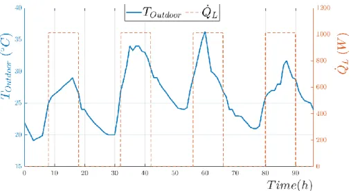
The climatic conditions of Montpellier, France, were selected and are representative of a
Mediterranean climate. Since it was harder to design the system for cooling purposes, a 4 day long hot
28 simply as a rectangular type signal. Its magnitude is 50 W per square meter of floor area from 8h to
18h, and set to zero otherwise. It is acknowledged that the reality is far more complex, but a simple
model for the heat loads was preferred in order to ease the comparison between the ventilated slabs
studied here.
Figure 13: Outdoor conditions and heat loads used for the test case
The temperature at the inlet of the slab Tin was set according to a simple control law, namely a fixed
temperature set point combined with hysteresis. Although this technique is simple, it is still quite
common for systems in building applications, even with TABS (Sourbron et al., 2009). Here, the
indoor set point was fixed at 22 ± 2 °C and Tin was set at 10 °C for cooling, 22 °C otherwise, as
illustrated in Figure 14. Air that enters in the TABS at 𝑇𝑖𝑛 is conditioned by the HVAC system. During
some short periods, the outdoor air is cooler than the indoor set point. Assuming the demand to be for
cooling only, a test was added to prevent the outdoor fresh air from being heated before being blown
into the ventilated slab. This was achieved by setting the inlet temperature to the outdoor temperature
when the latter was lower than the value obtained with the control law. For the sake of clarity, the
HVAC was not modeled and an ideal system was considered instead. By this, we mean that the
29
Figure 14: Control law used for setting the temperature at the inlet of the ventilated slab.
An adaptive time step technique was implemented in order to verify that dividing the time step by two
did not result in a difference higher than 10-3 °C on TRoom. All the simulations were initialized by
considering that both the room and the slab were at a homogeneous temperature (22 °C).
4.2. Non-ventilated slab model
For comparison, the thermal behavior of the room was assessed when a classical all by air system
(referred later as Non Ventilated Slab (NVS)) was used instead of a ventilated slab. As the heat
transfers were much simpler than for the ventilated slab, a classical 1D finite difference model with an
implicit time scheme was preferred to a state space model. The model was written with Matlab. It was
validated by comparing the results with the analytical solution for conductive heat transfer within a
semi-infinite solid, the upper face of which (z = 0) was subjected to a sinusoidal variation (Ozgener et
al., 2013). The temperature profile along the z direction, the z axis being downward, was given at any
time by: 𝑇(𝑧, 𝑡) = 𝑇̅̅̅ − 𝑇𝑢 ̂ 𝑒𝑢 −√ 𝜋 𝛼𝑇 𝑧𝑐𝑜𝑠 (2𝜋 𝑃 (𝑡 − 𝜏) − √ 𝜋 𝛼𝑃 𝑧) (23)
The average upper temperature 𝑇̅̅̅ and its amplitude 𝑇𝑢 ̂ were set to 20 and 5 °C, respectively. The 𝑢
period, P, was set to 1 year and the delay, τ, to zero. The thermal diffusivity, α, was set using the
30 years in order to obtain results that were independent of the initial conditions. The number of nodes
and the time step were tuned accordingly. The highest discrepancy was 7.10-3 °C, for a time selected
at random.
4.3. Results obtained for the reference case
The values computed for TRoom and Tin are plotted in Figure 15 for the reference case (ND = 9 and a
total air renewal of 6 ACH). This system was able to maintain the room temperature between 20 and
24 °C during the four days. Overall, the room temperature increased sharply in the morning, because
of the internal heat loads, until it reached 24 °C. Then, the temperature at the inlet of the ventilated
slab decreased to 10 °C, which helped to maintain the room temperature between 23 and 24 °C until
6 p.m. Note that Tin remained constant during this whole period, meaning that the HVAC system had
to run continuously to cool the room. At 6 p.m., the indoor temperature decreased suddenly as the heat
loads were set to zero. The temperature set point of the HVAC system remained the same for one more
hour, then the room temperature reached 20 °C and the temperature set point changed to 22 °C. As this
reference case was assumed to take place in summer, the HVAC system still had to provide cooling to
reach such a temperature, unless the outdoor air was cooler, in which case it was insufflated directly
into the ventilated slab. This technique is very simple and might not make best use of the thermal
inertia of the ventilated slab. Still, the room temperature increased slightly and remained lower than
22 °C until next morning, which is the target temperature for comfort. While more realistic techniques
could be implemented, those presented ease the analysis of the system and its comparison with
31
Figure 15: Room and inlet temperatures obtained for the reference case (left) and heat balance at the room scale for the fourth day (right).
Next, the heat fluxes used to compute the heat balance at the room scale according to (21) were
hour-averaged and are plotted in Figure 15 for the fourth day only. A positive value means that the
room is receiving a positive heat flux or that the room temperature is decreasing (because of the
negative sign on the term for indoor inertia in (21)).
From 9 a.m. to 6 p.m., the HVAC system provided cooling continuously in order to mitigate the
internal heat loads. The mean cooling power was -1.12 kW, approximately one third of which was
supplied to the room through the slab and the rest by the blown air. These ratios varied little over this
whole period. Note that they are close to the static gains ratio (40% and 60% for ND = 9).
When the heat loads were off, the magnitude of the heat fluxes at the room scale dropped to 0.1 kW.
The temperature at the inlet, Tin, was slightly above the room temperature, TRoom, because of the control
law used here. Consequently, the heat flux blown into the room, 𝑄̇𝐵 , was positive while the heat flux
exchanged with the slab, 𝑄̇𝑇 , was negative, meaning that the slab was still cooling the room. It is
acknowledged that more energy-efficient control laws could have been proposed. Nevertheless, indoor
conditions remained comfortable during the whole period.
4.4. Influence of the number of ducts and of the mass flow rate
The previous simulation work was repeated for the same scenario but with different numbers of ducts
32
Figure 16: Room temperature obtained with different number of ducts ND and with the
non-ventilated slab (NVS) under a constant air change rate (6 ACH).
The heat balance at the room scale was slightly affected by the number of ducts ND since the time and
duration for cooling were approximately the same. The indoor temperature, TRoom, remained within the
targeted range for all systems. However, it can be observed that increasing the number of ducts led to
less variable indoor temperatures, regardless of whether the heat loads were on or off. Also, the indoor
temperature remained closer to the threshold values (20 and 24 °C) when the number of ducts
increased. This is consistent with the previous conclusions that the amount of heat transmitted to the
room increases with the number of ducts. This favors thermal inertia and consequently smooths indoor
temperature variations. The non-ventilated slab had the same overall dimensions as the other systems,
but led to faster indoor temperature variation when the inlet temperature, Tin, changed. The result was
a slightly cooler indoor environment during the day and a hotter one during the night. The comparison
with the results obtained with the ventilated slab illustrates the increased thermal capacity brought by
the slab. Another interesting result is that comfortable indoor conditions were achieved by considering
a ventilated slab combined with a simple control law. Unlike the hydronic TABS, a significant fraction
of the heat flux blown into the slab was transmitted to the room almost instantaneously. On one hand,
it is harder to take full advantage of the thermal inertia of the slab but, on the other hand, it seemed
33 control of the system and avoid uncomfortable indoor conditions caused by a slow response to
unforeseen indoor temperature variations.
The influence of the mass flow rate was more pronounced than with varying ND, as depicted by Figure
17. While the room temperature was approximately the same at 8 a.m. for all systems, significant
differences were appearing as soon as the heat loads were on.
Figure 17: Room temperature obtained with different air change rates for a ventilated slab equipped with 9 ducts (VS) and a non-ventilated slab (NVS).
For the lowest air flow rate, the indoor temperature could not be maintained below 24 °C. In fact, it
never reached 20 °C during the four days, meaning that the HVAC system provided cooling
continuously. Despite the thermal inertia of the slab, it can be concluded that the cooling power
provided to the room was insufficient to meet the indoor temperature requirements when the air flow
rate was set at 2 ACH. Only minimal temperature differences were observed between the VS and the
NVS systems, which was not expected. As mentioned above, the heat flux transmitted through the slab
was higher at lower air flow rates, stressing the difference with a conventional system (here, an NVS).
However, this is not evident here. The reason for the difference lies in the mode of heat transfer, a
ventilated slab providing a more diffuse heat flux through the ceiling compared to an all-by-air system,
34 considering the high internal heat loads, the heat balance at the room scale was not greatly affected.
This statement tends to mitigate the idea that a low air flow rate should be used to take advantage of a
ventilated slab.
Increasing the mass flow rate to 10 ACH led to cooler indoor temperature when the heat loads are on.
For the VS, however, it can be observed that the HVAC system had to supply cooling almost
continuously from 8 a.m. to 6 p.m., which is very similar to what was obtained with 6 ACH. On the
other hand, the indoor temperature obtained with the NVS was more scattered during the day. As the
indoor temperature varies much faster, it reached the lower and the upper thresholds several times a
day, leading the HVAC system to be turned on and off repeatedly. This hardly ever happened with the
VS at the same air change rate, because of its additional thermal capacity.
To investigate a little further, the cooling demand was estimated with (24). The results were divided
by the value obtained for the reference case and are presented in Table 3.
𝐸 = ∫ 𝑚̇ 𝐶𝑎 𝑝,𝑎(𝑇𝑂𝑢𝑡𝑑𝑜𝑜𝑟− 𝑇𝑖𝑛) 𝑑𝑡 (24)
Table 3: Relative cooling demand for the 6 different cases
Air flow rate 6 ach 2 ach 10 ach
VS 1* 0.63 1.47
NVS 0.95 0.57 1.08
* Reference case
The results show the strong influence of the air change rate on the cooling demand. It could be roughly
approximated by a linear relationship for the VS: varying the air change rate by 1 ACH led to an
increase of about 10% in the energy consumption for this test case. However, for the non-ventilated
slab, this statement was no longer valid. For 10 ACH, the lower threshold was reached several times
during the day. In consequence, the HVAC provided less cooling for a while and the total energy
35 used here. For the other cases, the energy consumption was slightly lower than that obtained with a
ventilated slab. The reason is that, because of the increased inertia of the VS, there was still a cooling
demand at the end of the day, while there were no more heat loads. The opposite happened in the
morning but the time shift was smaller, leading to a higher cooling demand with VS than with NVS.
Obviously, the control law proposed here is usable with the NVS but it does not take advantage of the
additional thermal inertia of the ventilated slab and leads to higher energy consumption.
Overall, these results show that ND has a limited impact on the room temperature, yet increasing the
number of ducts is desirable in order to promote better indoor temperature stability. This conclusion
is important for practitioners as it means that the number of ducts is a parameter of lesser significance
that can be adjusted to fit on site constraints. On the other hand, the airflow rate has a significant
impact. While a low airflow rate favors heat transfer by conduction through the slab, there was little
difference on the heat balance of the room compared with a non-ventilated slab; the need to supply
cooling to the room in order to balance the heat loads still existed. This need defines a minimum air
flow rate that is required to achieve comfortable indoor temperatures. Increasing the airflow rate will
help this objective to be met but at the cost of a higher energy consumption. At the same time, the
influence of the control law is likely to be greater at higher airflow rates, and it should be tuned
carefully in order to avoid extra energy consumption.
4.5. Discussion
The methodology used here to obtain a lumped model for the ventilated slab was found to be adequate
for a fairly wide range of geometries and airflow rates. It strongly diminishes the computational time
for the heat transfer, allowing coupling with a room model. For the test case proposed here, the
computational time was approximately 1.5 s for a simulation period of one day.
There is a clear need to define an adequate airflow rate and a relevant command law for the ventilated
36 should be run for a longer period than four days in order to offer a wider range of outdoor conditions.
As the heat loads were found to have a significant impact on the indoor heat balance, they should be
modeled in greater detail. For example, they could include solar gains, which are time and orientation
specific. Also, a stochastic occupancy schedule could be used to be more realistic, as exemplified by
(Bui et al., 2019), among others. Finally, the HVAC system has to be modeled in order to give a more
accurate estimation of the energy consumption. It could include an energy recovery system on the
exhaust flow for example, which appears relevant as soon as the airflow rate increases. Moreover, the
cooling unit should be modeled so as to include a heat pump and its coefficient of performance (COP).
This would be relevant to test night-cooling strategies, as the COP increases during the night, when
the outdoor air is cooler.
The influence of the control law on the energy consumption was underlined by (Sourbron et al., 2009)
in the framework of a hydronic TABS, with a control law similar to the one used here. In practice,
such basic control laws are very common because they are easy to set up. Although the results
presented in this paper are limited to a narrow range of boundary conditions, they indicate that using
the same control law as for a non-ventilated slab did not result in major changes in terms of comfort
and energy consumption, as long as the air change rate was appropriate. This is an interesting result as
it questions the idea that a complex control strategy must necessarily be used with TABS, and could
help ventilated slabs to become more widely accepted.
Advanced control strategies, such as Model Predictive Control (MPC), are now mature and fulfill the
needs for reducing building energy consumption well (Ma et al., 2012). One such strategy has been
successfully applied to hydronic systems (Feng et al., 2015). It is recognized that this technique might
not be easy to implement on an existing HVAC system, as a retrofit may be required to deal with the
computational cost of this technique. On the other hand, it might bring interesting insight that would
allow a simple control law to be optimized. Further research should consider this kind of option in