HAL Id: hal-00952554
https://hal.inria.fr/hal-00952554v4
Submitted on 6 Oct 2014
HAL is a multi-disciplinary open access
archive for the deposit and dissemination of
sci-entific research documents, whether they are
pub-lished or not. The documents may come from
teaching and research institutions in France or
abroad, or from public or private research centers.
L’archive ouverte pluridisciplinaire HAL, est
destinée au dépôt et à la diffusion de documents
scientifiques de niveau recherche, publiés ou non,
émanant des établissements d’enseignement et de
recherche français ou étrangers, des laboratoires
publics ou privés.
Data-driven HRF estimation for encoding and decoding
models
Fabian Pedregosa, Michael Eickenberg, Philippe Ciuciu, Bertrand Thirion,
Alexandre Gramfort
To cite this version:
Fabian Pedregosa, Michael Eickenberg, Philippe Ciuciu, Bertrand Thirion, Alexandre Gramfort.
Data-driven HRF estimation for encoding and decoding models. NeuroImage, Elsevier, 2015, pp.209–220.
�10.1016/j.neuroimage.2014.09.060�. �hal-00952554v4�
Data-driven HRF estimation for encoding and decoding models
Fabian Pedregosa1,2,4,∗, Michael Eickenberg1,2,4, Philippe Ciuciu2,4, Bertrand Thirion2,4, AlexandreGramfort3,4
Abstract
Despite the common usage of a canonical, data-independent, hemodynamic response function (HRF), it is known that the shape of the HRF varies across brain regions and subjects. This suggests that a data-driven estimation of this function could lead to more statistical power when modeling BOLD fMRI data. However, unconstrained estimation of the HRF can yield highly unstable results when the number of free parameters is large. We develop a method for the joint estimation of activation and HRF by means of a rank constraint, forcing the estimated HRF to be equal across events or experimental conditions, yet permitting it to differ across voxels. Model estimation leads to an optimization problem that we propose to solve with an efficient quasi-Newton method, exploiting fast gradient computations. This model, called GLM with Rank-1 constraint (R1-GLM), can be extended to the setting of GLM with separate designs which has been shown to improve decoding accuracy in brain activity decoding experiments. We compare 10 different HRF modeling methods in terms of encoding and decoding score on two different datasets. Our results show that the R1-GLM model outperforms competing methods in both encoding and decoding settings, positioning it as an attractive method both from the points of view of accuracy and computational efficiency.
Keywords: Functional MRI (fMRI), Hemodynamic response function (HRF), machine learning,
optimization, BOLD, Finite inpulse response (FIR), decoding, encoding
1. Introduction
The use of machine learning techniques to predict the cognitive state of a subject from their functional MRI (fMRI) data recorded during task performance has become a popular analysis approach for neuroimag-ing studies over the last decade (Cox and Savoy, 2003; Haynes and Rees, 2006). It is now commonly referred to as brain reading or decoding. In this setting, the BOLD signal is used to predict the task or stimulus that the subject was performing. Although it is possible to perform decoding directly on raw BOLD sig-nal (Mour˜ao Miranda et al., 2007; Miyawaki et al., 2008), the common approach in fast event-related designs
∗Corresponding author. Email: [email protected]. Tel: +33 1 69 08 79 92 1
Authors contributed equally
2
Parietal Team, INRIA Saclay-ˆIle-de-France, Saclay, France
3
Institut Mines-Telecom, Telecom ParisTech, CNRS LTCI, 37-39 Rue Dareau, 75014 Paris, France
4
consists in extracting the activation coefficients (beta-maps) from the BOLD signal to perform the decoding analysis on these estimates. Similarly, in the voxel-based encoding models (Kay et al., 2008; Naselaris et al., 2011), the activation coefficients are extracted from the BOLD signal, this time to learn a model to predict the BOLD response in a given voxel, based on a given representation of the stimuli. In addition, a third approach, known as representational similarity analysis or RSA (Kriegeskorte et al., 2008) takes as input the activation coefficients. In this case a comparison is made between the similarity observed in the activation coefficients, quantified by a correlation measure, and the similarity between the stimuli, quantified by a similarity measure defined from the experimental setting.
These activation coefficients are computed by means of the General Linear Model (GLM) (Friston et al., 1995). While this approach has been successfully used in a wide range of studies, it does suffer from limi-tations (Poline and Brett, 2012). For instance, the GLM commonly relies on a data-independent canonical form of the hemodynamic response function (HRF) to estimate the activation coefficient. However it is known (Handwerker et al., 2004; Badillo et al., 2013b) that the shape of this response function can vary substantially across subjects and brain regions. This suggests that an adaptive modeling of this response function should improve the accuracy of subsequent analysis.
To overcome the aforementioned limitation, Finite Impulse Response (FIR) models have been proposed within the GLM framework (Dale, 1999; Glover, 1999). These models do not assume any particular shape for the HRF and amount to estimating a large number of parameters in order to identify it. While the FIR-based modeling makes it possible to estimate the activation coefficient and the HRF simultaneously, the increased flexibility has a cost. The estimator is less robust and prone to overfitting, i.e. to generalize badly to unseen data. In general, FIR models are most appropriate for studies focused on the characterization of the shape of the hemodynamic response, and not for studies that are primarily focused on detecting activation (Poldrack et al., 2011, Chapter 5).
Several strategies aiming at reducing the number of degrees of freedom of the FIR model - and thus at limiting the risk of overfitting - have been proposed. One possibility is to constrain the shape of the HRF to be a linear combination of a small number of basis functions. A common choice of basis is formed by three elements consisting of a reference HRF as well as its time and dispersion derivatives (Friston et al., 1998), although it is also possible to compute a basis set that spans a desired function space (Woolrich et al., 2004). More generally, one can also define a parametric model of the HRF and estimate the parameters that best fit this function (Lindquist and Wager, 2007). However, in this case the estimated HRF may no longer be a linear function of the input parameters.
Sensitivity to noise and overfitting can also be reduced through regularization. For example, temporal regularization has been used in the smooth FIR (Goutte et al., 2000; Ciuciu et al., 2003; Casanova et al., 2008) to favor solutions with small second order time derivative. These approaches require the setting of one or several hyperparameters, at the voxel or potentially at the parcel level (if several voxels in a pre-defined
parcel are assumed to share some aspects of the HRF timecourse). Even if efficient techniques such as generalized cross-validation (Golub et al., 1979) can be used to choose the regularization parameters, these methods are inherently more costly than basis-constrained methods. Basis-constrained methods also require setting the number of basis elements; however, this parameter is not continuous (as in the case of regularized methods), and in practice only few values are explored: for example the 3-element basis set formed by a reference HRF plus derivatives and the FIR model. This paper focuses on basis-constrained regularization of the HRF to avoid dealing with hyperparameter selection with the goal of remaining computationally attractive. A different approach to increase robustness of the estimates consists in linking the estimated HRFs across a predefined brain parcel, taking advantage of the spatially dependent nature of fMRI (Wang et al., 2013). However, hemodynamically-informed parcellations (Chaari et al., 2012; Badillo et al., 2013a) rely on the computation of a large number of estimations at the voxel or sub-parcel level. In this setting, the development of voxel-wise estimation procedures is complementary to the development of parcellation methods in that more robust estimation methods at the voxel level would naturally translate into more robust parcellation methods. In this paper we focus on voxel-wise estimation methods.
We propose a method for the simultaneous estimation of HRF and activation coefficients based on low-rank modeling. Within this model, and as in (Makni et al., 2008; Kay et al., 2008; Vincent et al., 2010; Degras and Lindquist, 2014), the HRF is constrained to be equal across the different conditions, yet permitting it to be different across voxels. Unlike previous works, we formulate this model as a constrained least squares problem, where the vector of coefficients is constrained to lie within the space of rank one matrices. We formulate the model within the framework of smooth optimization and use quasi-Newton methods to find the vector of estimates. This model was briefly presented in the conference paper (Pedregosa et al., 2013). Here we provide more experimental validation and a more detailed presentation of the method. We also added results using a GLM with separate designs (Mumford et al., 2012). Ten alternative approaches are now compared on two publicly available datasets. The solver has also been significantly improved to scale to full brain data.
The contributions of this paper are two-fold. First, we quantify the importance of HRF estimation in encoding and decoding models. While the benefit of data-driven estimates of the HRF have already been reported in the case of decoding (Turner et al., 2012) and encoding approaches (Vu et al., 2011), we here provide a comprehensive comparison of models. Second, we evaluate a method called GLM with
Rank-1 constraint (RRank-1-GLM) that improves encoding and decoding scores over state-of-the-art methods while
remaining computationally tractable on a full brain volume. We propose an efficient algorithm for this method and discuss practical issues such as initialization. Finally, we provide access to an open source software implementation of the methods discussed in this paper.
boldface letter to denote vectors and uppercase boldface letter to denote matrices. I denotes the identity matrix, 1n denotes the vector of ones of size n, ⊗ denotes the Kronecker product and vec(A) denotes the
concatenation of the columns of a matrix A into a single column vector. A† denotes the Moore-Penrose
pseudoinverse. Given the vectors {a1, . . . , ak} with ai ∈ Rn for each 1 ≤ i ≤ k, we will use the notation
[a1, . . . , ak] ∈ Rn×k to represents the columnwise concatenation of the k vectors into a matrix of size n × k.
We will use Matlab-style colon notation to denote slices of an array, that is x(1 : k) will denote the first k elements of x.
2. Methods
In this section we describe different methods for extracting the HRF and activation coefficients from BOLD signals. We will refer to each different stimulus as condition and we will call trial a unique presentation of a given stimulus. We will denote by k the total number of stimuli, y ∈ Rn the BOLD signal at a single
voxel and n the total number of images acquired.
2.1. The General Linear Model
The original GLM model (Friston et al., 1995) makes the assumption that the hemodynamic response is a linear transformation of the underlying neuronal signal. We define the n×k-matrix XGLMas the columnwise
stacking of different regressors, each one defined as the convolution of a reference HRF (Boynton et al., 1996; Glover, 1999) with the stimulus onsets for the given condition. In this work we used as reference HRF the one provided by the software SPM 8 (Friston et al., 2011). Assuming additive white noise, n ≥ k and XGLM to be full rank, the vector of estimates is given by ˆβGLM = X
†
GLMy, where ˆβGLM is a vector of size
k representing the amplitude of each one of the conditions in a given voxel.
A popular modification of this setting consists in extending the GLM design matrix with the temporal and width derivatives of the reference HRF. This basis, formed by the reference HRF and its derivatives with respect to time and width parameters, will be used throughout this work. We will refer to it as the 3HRF
basis. In this case, each one of the basis elements is convolved with the stimulus onsets of each condition,
obtaining a design matrix of size n × 3k. This way, for each condition, we estimate the form of the HRF as a sum of basis functions that correspond to the first order Taylor expansion of the parametrization of the response function. Another basis set that will be used is the Finite Impulse Response (FIR) set. This basis set spans the complete ambient vector space (of dimension corresponding to the length of the impulse response) and it is thus a flexible model for capturing the HRF shape. It consists of the canonical unit vectors (also known as stick function) for the given duration of the estimated HRF. Other basis functions such as FMRIB’s Linear Optimal Basis Sets (Woolrich et al., 2004) are equally possible but were not considered in this work.
More generally, one can extend this approach to any set of basis functions. Given the matrix formed by the stacking of d basis elements B = [b1, b2, . . . , bd], the design matrix XB is formed by successively
stacking the regressors obtained by convolving each of the basis elements with the stimulus onsets of each condition. This results in a matrix of size n × dk and under the aforementioned conditions the vector of estimates is given by ˆβB = X†By. In this case, ˆβB is no longer a vector of size k: it has length k × d instead and can no longer be interpreted as the amplitude of the activation. One possibility to recover the trial-by-trial reponse amplitude is to select the parameters from a single time point as done by some of the models considered in (Mumford et al., 2012), however this procedure assumes that the peak BOLD response is located at that time point. Another possibility is to construct the estimated HRF and take as amplitude coefficient the peak amplitude of this estimated HRF. This is the approach that we have used in this paper.
2.2. GLM with rank constraint
In the basis-constrained GLM model, the HRF estimation is performed independently for each condition. This method works reliably whenever the number of conditions is small, but in experimental designs with a large number of conditions it performs poorly due to the limited conditioning of the problem and the increasing variance of the estimates.
At a given voxel, it is expected that for similar stimuli the estimated HRF are also similar (Henson et al., 2002). Hence, a natural idea is to promote a common HRF across the various stimuli (given that they are sufficiently similar), which should result in more robust estimates (Makni et al., 2008; Vincent et al., 2010). In this work we consider a model in which a common HRF is shared across the different stimuli. Besides the estimation of the HRF, a unique coefficient is obtained per column of our event matrix. This amounts to the estimation of k + d free parameters instead of k × d as in the standard basis-constrained GLM setting. The novelty of our method stems from the observation that the formulation of the GLM model with a common HRF across conditions translates to a rank constraint on the vector of estimates. This assumption amounts to enforcing the vector of estimates to be of the form βB = [hβ1, hβ2, · · · , hβk] for some HRF
h∈ Rd and a vector of coefficients β ∈ Rk. More compactly, this can be written as β
B= vec(hβ T
). This can be seen as a constraint on the vector of coefficients to be the vectorization of a rank-one matrix, hence the name Rank-1 GLM (R1-GLM).
In this model, the coefficients have no longer a closed form expressions, but can be estimated by minimiz-ing the mean squared error of a bilinear model. Given XBand y as before, Z ∈ Rn×q a matrix of nuisance
parameters such as drift regressors, we define FR1(h, β, ω, XB, y, Z) = 12ky − XBvec(hβ T
) − Zωk2 to be
the objective function to be minimized. The optimization problem reads: ˆ
h, ˆβ, ˆω = arg min
h,β,ω
FR1(h, β, ω, XB, y, Z)
subject to kBhk∞= 1 and hBh, hrefi > 0 ,
The norm constraint is added to avoid the scale ambiguity between h and β and the sign is chosen so that the estimated HRF correlates positively with a given reference HRF href. Otherwise the signs of the HRF
and β can be simultaneously flipped without changing the value of the cost function. Within its feasible set, the optimization problem is smooth and is convex with respect to h, β and ω, however it is not jointly
convex in variables h, β and ω.
From a practical point of view this formulation has a number of advantages. First, in contrast with the GLM without rank-1 constraint the estimated coefficients are already factored into the estimated HRF and the activation coefficients. That is, once the estimation of the model parameters from Eq. (1) is obtained, ˆβ is a vector of size k and ˆhis a vector of size d that can be both used in subsequent analysis, while in models without rank-1 constraint only the vector of coefficients (equivalent to vec(hβT) in rank-1 constrained models) of size k × d is estimated. In the latter case, the estimated HRF and the beta-maps still have to be extracted from this vector by methods such as normalization by the peak of the HRF, averaging or projecting to the set of Rank-1 matrices.
Second, it is readily adapted to prediction on unseen trials. While for classical (non rank-1 models) the HRF estimation is performed per condition with no HRF associated with unseen conditions, in this setting, because the estimated HRF is linked and equal across conditions it is natural to use this estimate on unseen conditions. This setting occurs often in encoding models where prediction on unseen trials is part of the cross-validation procedure.
This model can also be extended to a parametric HRF model. That is, given the hemodynamic response defined as a function h : Rd1 → Rdof some parameters α, we can formulate the analogous model of Eq. (1)
as an optimization over the parameters α and β with the design matrix XFIR given by the convolution of
the event matrix with the FIR basis: ˆ
α, ˆβ, ˆω = arg min
α,β,ω
FR1(h(α), β, ω, XFIR, y, Z)
subject to kh(α)k∞= 1 and hh(α), hrefi > 0
(2)
In section 2.4 we will discuss optimization strategies for both models.
2.3. Extension to separate designs
An extension to the classical GLM that improves the estimation with correlated designs was proposed in (Mumford et al., 2012). In this setting, each voxel is modeled as a linear combination of two regressors in a design matrix XGLM. The first one is the regressor associated with a given condition and the second one
is the sum of all other regressors. This results in k design matrices, one for each condition. The estimate for a given condition is given by the first element in the two-dimensional array XSi†y, where XSi is the design
to find a better estimate in rapid event designs leading to a boost in accuracy for decoding tasks (Mumford et al., 2012; Schoenmakers et al., 2013; Lei et al., 2013).
This approach was further extended in (Turner et al., 2012) to include FIR basis instead of the predefined canonical function. Here we employ it in the more general setting of a predefined basis set. Given a set of basis functions we construct the design matrix for condition i as the columnwise concatenation of two matrices X0
BSi and X 1 BSi. X
0
BSi is given by the columns associated with the current condition in the GLM
matrix and X1
BSi is the sum of all other columns. In this case, the vector of estimates is given by the first d
vectors of X†BSiy. See (Turner et al., 2012) for a more complete description of the matrices X 0
BSiand X 1 BSi.
It is possible to use the same rank-1 constraint as before in the setting of separate designs, linking the HRF across conditions. We will refer to this model as Rank-1 GLM with separate designs (R1-GLMS). In this case the objective function has the form FR1-S(h, β, ω, r, XB, y, Z) =12Pki ky−βiX0BSih−riX1BSih−Zωk2,
where r ∈ Rdis a vector representing the activation of all events except the event of interest and will not be
used in subsequent analyses. We can compute the vector of estimates ˆβas the solution to the optimization problem
ˆ
β, ˆω, ˆh, ˆr = arg min
h,β,ω,r
FR1-S(h, β, ω, r, XB, y, Z)
subject to kBhk∞= 1 and hBh, hrefi > 0
(3)
2.4. Optimization
For the estimation of rank-1 models on a full brain volume, a model is estimate at each voxel separately. Since a typical brain volume contains more than 40,000 voxels, the efficiency of the estimation at a single voxel is of great importance. In this section we will detail an efficient procedure based on quasi-Newton methods for the estimation of R1-GLM and R1-GLMS models on a given voxel.
One approach to minimize (1) is to alternate the minimization with respect to the variables β, h and ω. By recalling the Kronecker product identities (Horn and Johnson, 1991, Chapter 4.3), and using the identity vec(hβT) = β ⊗ h we can rewrite the objective function (1) to be minimized as:
1 2ky − XB(β ⊗ h) − Zωk 2 = 1 2ky − XB(I ⊗ h)β − Zωk 2 = 1 2ky − XB(β ⊗ I)h − Zωk 2 . (4)
Updating h, β or ω sequentially thus amounts to solving a (constrained) least squares problem at each iteration. A similar procedure is detailed in (Degras and Lindquist, 2014). However, this approach requires computing the matrices XB(β ⊗ I) and XB(I ⊗ h) at each iteration, which are typically dense, resulting in a high computational cost per iteration. Note also that the optimization problem is not jointly convex in variables h, β, ω, therefore we cannot apply convergence guarantees from convex analysis.
We rather propose a more efficient approach by optimizing both variables jointly. We define a global variable z as the concatenation of (h, β, ω) into a single vector, z = vec([h, β, ω]), and cast the problem
as an optimization with respect to this new variable. Generic solvers for numerical optimization (Nocedal and Wright, 2006) can then be used. The solvers that we will consider take as input an objective func-tion and its gradient. In this case, the partial derivatives with respect to variable z can be written as ∂FR1/∂z = vec([∂FR1/∂h, ∂FR1/∂β, ∂FR1/∂ω]), whose expression can be easily derived using the
afore-mentioned Kronecker product identities: ∂FR1 ∂h = − (β T ⊗ I)XT(y − X vec(hβT ) − Zω) ∂FR1 ∂β = − (I ⊗ h T )XT(y − X vec(hβT) − Zω) ∂FR1 ∂ω = − Z T(y − X vec(hβT ) − Zω)
If instead a parametric model of the HRF is used as in Eq. (2), the equivalent partial derivatives can be easily computed by the chain rule.
For the sake of efficiency, it is essential to avoid evaluating the Kronecker products naively, but rather reformulate them using the above mentioned Kronecker identities. For example, the matrix M = X(I ⊗ h) should not be computed explicitly but should rather be stored as a linear operator such that when applied to a vector a ∈ Rk it computes M (a) = X(a ⊗ h), avoiding thus the explicit computation of I ⊗ β.
Similar equations can be derived for the rank-1 model with separate designs of Eq. (3) (R1-GLMS), in which case the variable z is defined as the concatenation of (h, β, ω, r), i.e. z = vec([h, β, ω, r]). The gradi-ent of FR1-Swith respect to z can be computed as ∂FR1-S/∂z = vec([∂FR1-S/∂h, ∂FR1-S/∂β, ∂FR1-S/∂ω, FR1-S/∂r]).
The partial derivatives read: ∂F ∂h = Pk i −(X 0 BSiβi− X 1 BSiri) T(y − β iX0BSih − wiX 1 BSih) ∂F ∂βi = −(X 0 BSih) T(y − β iX0BSih− wiX 1 BSih) ∂F ∂ωi = −Z T(y − β iX0BSih− wiX 1 BSih) ∂F ∂ri = −(X 1 BSih) T(y − β iX0BSih− wiX 1 BSih)
A good initialization plays a crucial role in the convergence of any iterative algorithm. Furthermore, for non-convex problems a good initialization prevents the algorithm from converging to undesired local minima. We have used as initialization for the R1-GLM and R1-GLMS models the solution given by the GLM with separate designs (GLMS). Since the GLM with separate designs scales linearly in the number of voxels, this significantly reduces computation time whenever an important number of voxels is considered.
Whenever the design matrix XBhas more rows than columns (as is the case in both datasets we consider with B the 3HRF basis), it is possible to find an orthogonal transformation that significantly speeds up the computation of the Rank-1 model. Let Q, R be the “thin” QR decomposition of XB ∈ Rn×dk, that is,
QR= XB with Q ∈ Rn×dk an orthogonal matrix and R ∈ Rdk×dk a triangular matrix. Because of the
invariance of the Euclidean norm to orthogonal transformations, the change of variable XB ← QTXB,
matrix to a square triangular matrix of size dk × dk (instead of n × dk) and reduces the explained variable yto a vector of size kd (instead of n). After this change of variable, the convergence of the Rank-1 model is significantly faster due to the faster computation of the objective function and its partial derivatives. We have observed that the total running time of the algorithm can be reduced by 30% using this transformation. Some numerical solvers such as L-BFGS-B (Liu and Nocedal, 1989) require the constraints to be given as box constraints. While our original problem includes an equality constraint we can easily adapt it to use convex box constraints instead. We replace the equality constraint kBhk∞ = 1 by the convex inequality
constraint kBhk∞ ≤ 1, which is equivalent to the box constraint −1 ≤ (Bh)i ≤ 1 supported by the
above solver. However, this change of constraint allows solutions in which h can be arbitrarily close to zero. To avoid such degenerate cases we add the smooth term −kBhk2
2 to the cost function. Since there
is a free scale parameter between h and β, this does not bias the problem, but forces Bh to lie as far as possible from the origin (thus saturating the box constraints). Once a descent direction has been found by the L-BFGS-B method we perform a line search procedure to determine the step length. The line-search procedure was implemented to satisfy the strong Wolfe conditions (Nocedal and Wright, 2006). Finally, when the optimization algorithm has converged to a stationary point, we rescale the solution setting to ensure that the equality constraint. This still leaves a sign ambiguity between the estimated HRF and the associated beta-maps. To make these parameters identifiable, the sign of the estimated HRF will be chosen so that these correlate positively with the reference HRF.
We have compared several first-order (Conjugate Gradient), quasi-Newton (L-BFGS) and Newton meth-ods on this problems and found that in general quasi-Newton methmeth-ods performed best in terms of compu-tation time. In our implemencompu-tation, we adopt the L-BFGS-B as the default solver.
In Algorithm 1 we describe an algorithm based on L-BFGS that can be used to optimize R1-GLM and R1-GLMS models (a reference implementation for the Python language is described in subsection Software). Variable r is only used for the R1-GLMS method and its use is denoted within parenthesis, i.e. (, r), so that for the R1-GLM it can simply be ignored.
The full estimation of the R1-GLM model with 3HRF basis for one subject of the dataset described in section Dataset 2: decoding of potential gain levels (16 × 3 conditions, 720 time points, 41, 622 voxels) took 14 minutes in a 8-cores Intel Xeon 2.67GHz machine. The total running time for the 17 subjects was less than four hours.
2.5. Software
We provide a software implementation of all the models discussed in this section in the freely available (BSD licensed) pure-Python package hrf estimation5.
5
Algorithm 1Optimization of R1-GLM and R1-GLMS models Input: Given initial points β0 ∈ R
k, h
0 ∈ Rd, ω0 ∈ Rq (, r0 ∈ Rk), convergence tolerance ǫ > 0, inverse
Hessian approximation H0.
Output: βm, hm
1: (Optional): Compute the QR decomposition of XB, QR = XB, and replace XB← QTXB, y ← QTy
2: Initialization. Set m ← 0, z ← vec([h0, β0, ω0(, r0)])
3: while k∇f k > ǫ do
4: Compute search direction. Set pm ← −Hm∇f (hm, βm, ωm(, rm)) by means of the L-BFGS
algo-rithm.
5: Set zm+1 = zm+ γmpm, where γm is computed from a line search procedure subject to the box
constraints khmk∞≤ 1.
6: m ← m + 1
7: end while
8: Extract R1-GLM(S) parameters from zm. Set hm← zm(1 : d), βm← zm(d + 1 : m + d)
9: Normalize and set sign so that the estimated HRF is positively correlated with a reference HRF: qm←
khmk∞sign(hTmhref), hm← hm/qm, βm← βmqm
3. Data description
With the aim of making the results in this paper easily reproducible, we have chosen two freely available datasets to validate our approach and to compare different HRF modeling techniques.
3.1. Dataset 1: encoding of visual information
The first dataset we will consider is described in (Kay et al., 2008; Naselaris et al., 2009; Kay et al., 2011). It contains BOLD fMRI responses in human subjects viewing natural images. As in (Kay et al., 2008), we performed prediction of BOLD signal following the visual presentation of natural images and compared it against the measured fMRI BOLD signal. As the procedure consists of predicting the fMRI data from stimuli descriptors, it is an encoding model. This dataset is publicly available from http://crcns.org
Two subjects viewed 1750 training images, each presented twice, and 120 validation images, each pre-sented 10 times, while fixating a central cross. Images were flashed 3 times per second (200 ms on-off-on-off-on) for one second every 4 seconds, leading to a rapid event-related design. The data were acquired in 5 scanner sessions on 5 different days, each comprising 5 runs of 70 training images –each image being presented twice within the run– and 2 runs of validation images showing 12 images, 10 times each. The images were recorded from the occipital cortex at a spatial resolution of 2mm×2mm×2.5mm and a temporal resolution of 1 second. Every brain volume for each subject has been aligned to the first volume of the first run of the first session for that subject. Across-session alignment was performed manually. Additionally,
data were temporally interpolated to account for slice-timing differences. See (Kay et al., 2008) for further preprocessing details.
We performed local detrending using a Savitzky-Golay filter (Savitzky and Golay, 1964) with a poly-nomial of degree 4 and a window length of 91 TR. The activation coefficients (beta-map) and HRF were extracted from the training set by means of the different methods we would like to compare. The training set consisted of 80% of the original session (4 out of 5 runs). This resulted in estimated coefficients (beta-map) for each of the 70 × 4 images in the training set.
We proceed to train the encoding model. The stimuli are handled as local image contrasts, that are represented by spatially smoothed Gabor pyramid transform modulus with 2 orientations and 4 scales. Ridge regression (regularization parameter chosen by Generalized Cross-Validation (Golub et al., 1979)) was then used to learn a predictor of voxel activity on the training set. By using this encoding model and the estimated HRF it is possible to predict the BOLD signal for the 70 images in the test set (20 % of the original session). We emphasize that learning the HRF on the training set instead of on the full dataset is necessary to avoid overfitting while assessing the quality of the estimated HRF by any HRF-learning method: otherwise, the estimation of the HRF may incorporate specificities of the test set leading to artificially higher scores.
In a first step, we perform the image identification task from (Kay et al., 2008). From the training set we estimate the activation coefficients that will be used to compute the activation maps. We use an encoding model using Gabor filters that predicts the activation coefficient from the training stimuli. From the stimuli in the validation set we predict the activation coefficients that we then use to identify the correct image. The predicted image is the one yielding the highest correlation with the measured activity. This procedure mimics the one presented in (Kay et al., 2008, Supplementary material).
In a second step, we report score as the Pearson correlation between the measurements and the predicted BOLD signal on left out data. The prediction of BOLD signal on the test set is performed from conditions that were not present in the train set. In order to do this, an HRF for these conditions is necessary. As highlighted in the methods section, the construction of an HRF for these conditions is ambiguous for non Rank-1 methods that perform HRF estimation on the different stimuli. In these cases we chose to use the mean HRF across conditions as the HRF for unseen conditions. Finally, linear predictions on the left out fold were compared to the measured BOLD signals.
3.2. Dataset 2: decoding of potential gain levels
The second dataset described in (Tom et al., 2007) is a gambling task where each of the 17 subjects was asked to accept or reject gambles that offered a 50/50 chance of gaining or losing money. The magnitude of the potential gain and loss was independently varied across 16 levels between trials. Each gamble has an amount of potential gains and potential losses that can be used as class label. In this experiment, we only
considered gain levels. This leads to the challenge of predicting or decoding the gain level from brain images. The dataset is publicly available from http://openfmri.org under the name mixed-gambles task dataset.
The data preprocessing included slice timing, motion correction, coregistration to the anatomical images, tissue segmentation, normalization to MNI space and was performed using the SPM 8 software through the Pypreprocess6interface.
For all subjects three runs were recorded, each consisting of 240 images with a repetition time (TR) of 2 seconds and a stimulus presentation at every 4 seconds. In order to perform HRF estimation on more data than what is available on a single run, we performed the estimation on the three runs simultaneously. This assumes HRF consistency across runs, which was obtained by concatenating the data from the three runs and creating a block-diagonal design matrix correspondingly (each block is the design of one run).
After training a regression model on 90% of the data, we predict the gain level on the remaining 10%. As a performance measure we use Kendall tau rank correlation coefficient (Kendall, 1938) between the true gain levels and the predicted levels, which is a measure for the orderings of the data. We argue that this evaluation metric is better suited than a regression loss for this task because of the discrete and ordered nature of the labels. Also, this loss is less sensible to shrinkage of the prediction that might occur when penalizing a regression model (Bekhti et al., 2014). The Kendall tau coefficient always lies within the interval [−1, 1], with 1 being perfect agreement between the two rankings and −1 perfect disagreement. Chance level lies at zero. This metric was previously proposed for fMRI decoding with ordered labels in (Doyle et al., 2013).
4. Results
In order to compare the different methods discussed previously, we ran the same encoding and decoding studies while varying the estimation method for the activation coefficients (beta-maps). The methods we considered are standard GLM (denoted GLM), GLM with separate designs (GLMS), Rank-1 GLM (R1-GLM) and Rank-1 GLM with separate designs (R1-GLMS). For all these models we consider different basis sets for estimating the HRF: a set of three elements formed by the reference HRF and its time and dispersion derivative, a FIR basis set (of size 20 in the first dataset and of size 10 in the second dataset) formed by the canonical vectors and the single basis set formed by the reference HRF (denoted “fixed HRF”), which in this case is the HRF used by the SPM 8 software.
It should be reminded that the focus of this study is not the study of the HRF in itself (such as variability across subjects, tasks or regions) but instead its possible impact on the accuracy of encoding and decoding paradigms. For this reason we report encoding and decoding scores but we do not investigate any of the possible HRF variability factors.
6
4.1. Dataset 1: encoding of visual information
In the original study, 500 voxels were used to perform image identification. These voxels were selected as the voxels with the highest correlation with the true BOLD signal on left-out data using a (classical) GLM with the reference HRF. These voxels are therefore not the ones naturally benefiting the most from HRF estimation.
We first present the scores obtained in the image identification task for different variants of the GLM. This can be seen in Figure 1. The displayed score is the count of correctly identified images over the total number of images (chance level is therefore at 1/120). The identification algorithm here only uses the beta-maps obtained from the train and validation set. This makes the estimation of the HRF an intermediate result in this model. However, we expect that a correct estimation of the HRF directly translates into a better estimation of the activation coefficients in the sense of being able to acheive higher predictive accuracy. Our results are consistent with this hypothesis and in this task the rank-one (R1) and glm-separate (GLMS) models outperform the classical GLM model. The benefits range from 0.9% for R1-GLM in subject 2 to 8.2% for the same method and subject 1. It is worth noticing that methods with FIR basis obtain a higher score than methods using the 3HRF basis.
In order to test whether this increase is statistically significant we performed the following statistical test. The success of recovering the correct image can be modeled as a binomial distribution, with pA being
be the probability of recovering the correct image with method A and pB be the probability of recovering
the correct image with method B. We define the null hypothesis H0as the statement that both probabilities
are equal, H0: pA= pB, and the alternate hypothesis that both probabilities and not equal, H1: p16= p2
(this test is sometimes known as the binomial proportion test (R¨ohmel and Mansmann, 1999)). The score test statistic for the one-tailed test is T = (pA− pB)/
q
p(1 − p)2
n, where p = (pA+ pB)/2 and n is the
number of repetitions, in this case n = 120. This statistic is normally distributed for large n. The p-value associated with this statistical test when comparing every model (by order of performance) with the model “GLM with with fixed HRF” is (0.10, 0.10, 0.15, 0.19, 0.21, 0.26, 0.5, 0.5, 0.82, 0.81) for the first subject and (0.18, 0.18, 0.25, 0.34, 0.34, 0.44, 0.5, 0.5, 0.86, 0.93) for the second.
We will now use a different metric for evaluating the performance of the encoding model. This metric is the Pearson correlation between the BOLD predicted by the encoding model and the true BOLD signal, averaged across voxels. We will compute the this metric on a left-out session, which results in five scores for each method, corresponding to each of the cross-validation folds. Given two methods, a Wilcoxon signed-rank test can be used on these cross-validation scores to assess whether the score obtained by the two methods are significantly different. This way, irrespective of the variance across voxels, which is inherent to the study, we can reliably assess the relative ranking of the different models. In Figure 2 we show the scores for each method (averaged across sessions) and the p-value corresponding the Wilcoxon test between a given method and the previous one by order of performance.
GLM with FIR basis GLM with 3HRF basis GLM with fixed HRF GLMS with fixed HRF R1-GLMS with 3HRF basis R1-GLM with 3HRF basis R1-GLMS with FIR basis GLMS with 3HRF basis GLMS with FIR basis R1-GLM with FIR basis
0.460 0.467 0.518 0.518 0.558 0.568 0.575 0.583 0.600 0.600
Image Identification Performance, subject 1
R1-GLMS R1-GLM
GLMS GLM
GLM with FIR basis
GLM with 3HRF basis
GLM with fixed HRF
GLMS with fixed HRF
R1-GLM with 3HRF basis
GLMS with FIR basis
R1-GLM with FIR basis
R1-GLMS with 3HRF basis
GLMS with 3HRF basis
R1-GLMS with FIR basis
0.416
0.446
0.516
0.516
0.525
0.541
0.541
0.558
0.575
0.575
Image Identification Performance, subject 2
R1-GLMS R1-GLM
GLMS GLM
Figure 1: Image identification score (higher is better) on two different subjects from the first dataset. The metric counts the number of correctly identified images over the total number of images (chance level is 1/120 ≈ 0.008). This metric is less sensitive to the shape of the HRF than the voxel-wise encoding score. The benefits range from 0.9% points to 8.2% points across R1-constrained methods and subjects. The highest score is achieved by a R1-GLM method with a FIR basis set for subject 1 and by a R1-GLMS with FIR basis for subject 2.
GLM with FIR basis GLM with fixed HRF GLMS with fixed HRF GLM with 3HRF basis GLMS with 3HRF basis R1-GLM with 3HRF basis R1-GLMS with 3HRF basis GLMS with FIR basis R1-GLMS with FIR basis R1-GLM with FIR basis
0.011 0.058 *** 0.063 *** 0.067 ** 0.149 *** 0.168 *** 0.185 *** 0.204 *** 0.216 0.219 *** p-value = *< 0.05, **< 10−3, ***< 10−6
Average Correlation Score, subject 1
R1-GLMS R1-GLM
GLMS GLM
GLM with FIR basis GLM with fixed HRF GLM with 3HRF basis GLMS with fixed HRF GLMS with 3HRF basis R1-GLM with 3HRF basis R1-GLMS with 3HRF basis R1-GLM with FIR basis GLMS with FIR basis R1-GLMS with FIR basis
0.011 0.064 *** 0.064 0.069 ** 0.147 *** 0.156 ** 0.181 *** 0.194 *** 0.202 *** 0.223 *** p-value = *< 0.05, **< 10−3, ***< 10−6
Average Correlation Score, subject 2
R1-GLMS R1-GLM
GLMS GLM
Figure 2: Average correlation score (higher is better) on two different subjects from the first dataset. The average correlation score is the Pearson correlation between the predicted BOLD and the true BOLD signal on left-out session, averaged across voxels and sessions. Methods that perform constrained HRF estimation significantly outperform methods that use a fixed reference HRF. As for the image identification performance, the best performing method for subject 1 is the R1-GLM, while for subject 2 it is the R1-GLMS model, both with FIR basis. In underlined typography is the GLM with a fixed HRF which is the method used by default in most software distributions. A Wilcoxon signed-rank test is performed between each method and the next one in the ordered result list by considering the leave-one-session out cross-validation scores for each method. We report p-values to assess whether the score differences are statistically significant.
We observed in Figure 2 that methods that learn the HRF together with some sort of regularization (be it Rank-1 constraint or induced by separate designs) perform noticeably better than methods that perform unconstrained HRF estimation, highlighting the importance of a robust estimation of the HRF as opposed to a free estimation as performed by the standard GLM model with FIR basis. This suggests that R1 and GLMS methods permit including FIR basis sets while minimizing the risk of overfitting inherent to the classical GLM model.
We also observed that models using the GLM with separate designs from (Mumford et al., 2012) perform significantly better on this dataset than the standard design, which is consistent with the purpose of these models. It improves estimation in highly correlated designs. The best performing model for both subjects in this task is the R1-GLMS with FIR basis, followed by the R1-GLM with FIR basis model for subject 1 and GLMS with FIR basis for subject 2. The difference between both models (Wilcoxon signed-rank test) was significant with a p-value < 10−6. Since the results for both subjects are similar, we will only use subject 1
for the rest of the figures.
To further inspect the results, we investigated the estimation and encoding scores at the voxel level. This provides some valuable information. For example, parameters such as time-to-peak, width and undershoot of the estimated HRF can be used to characterize the mis-modeling of a reference HRF for the current study. Also, a voxel-wise comparison of the different methods can be used to identify which voxels exhibit a greater improvement for a given method. In the upper part of Figure 3 we show the HRF estimated on the first subject by our best performing method (the Rank-1 with separate designs and FIR basis). For comparison we also present two commonly used reference HRFs: one used in the software SPM and one defined in (Glover, 1999, auditory study) and used by software such as NiPy7 and fmristat8. Because the
HRF estimation will fail on voxels for which there is not enough signal, we only show the estimated HRF for voxels for which the encoding score is above the mean encoding score. In this plot the time-to-peak of the estimated HRF is color coded. One can observe a substantial variability in the time to peak, confirming the existence of a non-negligeable variability of the estimated HRFs, even within a single subject and a single task. In particular, we found that only 50% of the estimated HRFs on the full brain volume peaked between 4.5 and 5.5 seconds.
In the lower part of Figure 3 we can see a scatter plot in which the coordinates of each point are the encoding scores with two different methods. The first coordinate (X-axis) is given by the score using a canonical GLM whilst the second coordinate (Y-axis) corresponds to the Rank-1 separate with FIR basis. Points above the black diagonal exhibit a higher score with our method than with a canonical GLM. As previously, the color represents the time to peak of the estimated HRF. From this plot we can see that voxels that have a low correlation score using a canonical GLM do not gain significant improvement by using a
7
http://nipy.org
8
Figure 3: Top: HRF estimated by the R1-GLMS method on voxels for which the encoding score was above the mean encoding score (first dataset), color coded according to the time to peak of the estimated HRFs. The difference in the estimated HRFs suggests a substantial variability at the voxel level within a single subject and a single task. Bottom: voxel-wise encoding score for the best performing method (R1-GLMS with FIR basis) versus a standard GLM (GLM with fixed HRF) across voxels. The metric is Pearson correlation. Points above the black diagonal correspond to voxels that exhibit a higher score with the R1-GLMS method than with a standard GLM.
Rank-1 Separate FIR model instead. However, voxels that already exhibit a sufficiently high correlation score using a canonical GLM (> 0.05) see a significant increase in performance when estimated using our method.
These results suggest as a strategy to limit the computational cost of learning the HRF on an encoding study to perform first a standard GLM (or GLMS) on the full volume and then perform HRF estimation only on the best performing voxels.
The methods that we have considered for HRF estimation can be subdivided according to the design matrices they use (standard or separate) and the basis they use to generate the estimated HRF (3HRF and FIR). We now focus on the performance gains of each of these individual components. In the upper part of Figure 4 we consider the top-performing model, the Rank-1 GLMS, and compare the performance of two different basis sets: FIR with 20 elements in the Y-axis and the reference HRF plus its time and dispersion derivatives (3HRF) in the X-axis. The abundance of points above the diagonal demonstrates the superiority of the FIR basis on this dataset. The color trend in this plot suggests that the score improvement of the FIR basis with respect to the 3HRF basis becomes more pronounced as the time-to-peak of the estimated HRF deviates from the reference HRF (peak at 5s), which can be explained by observing that the 3HRF basis corresponds to a local model around the time-to-peak. In the bottom part of this figure we compare the different design matrices (standard or separate). Here we can see the voxel-wise encoding score for two Rank-1 models with FIR basis and different design matrices: separate design on the Y-axis and classical design on the X-axis. Although both models give similar results, a Wilcoxon signed-rank test on the leave-one-session-out cross-validation score confirmed the superiority of the separate designs model in this dataset with p-value < 10−3.
In Figure 5 we can see the voxel-wise encoding score on a single acquisition slice. In the upper column, the score is plotted on each voxel and thresholded at a value of 0.045, which would correspond to a p-value < 0.05 for testing non-correlation assuming each signal is normally distributed, while in the bottom row the 0.055 contour (p-value < 0.001) for the same data is shown as a green line. Here it can be seen how the top performing voxels follow the gray matter. A possible hypothesis to explain the increase of the encoding score between the method R1-GLMS with FIR basis and the same method with 3HRF basis could be related either to the shape of the HRF deviating more from a canonical shape in lateral visual areas or to the higher signal-to-noise ratio often found in the visual cortex when compared to lateral visual areas.
4.2. Dataset 2: decoding of potential gain levels
The mean decoding score was computed over 50 random splittings of the data, with a test set of size 10%. The decoding regression model consisted of univariate feature selection (ANOVA) followed by a Ridge regression classifier as implemented in scikit-learn (Pedregosa et al., 2011). Both parameters, number of voxels and amount of ℓ2regularization in Ridge regression, were chosen by cross-validation.
Figure 4: Voxel-wise encoding score for different models that perform HRF estimation (first dataset). As in figure 3, color codes for the time to peak of the estimated HRF at the given voxel. Top: two Rank-1 separate design models with different basis functions: FIR with 20 elements in the Y-axis and the reference HRF with its time and dispersion derivatives (3HRF) in the X-axis. The color trend in this plot suggests that the score improvement of the FIR basis with respect to the 3HRF becomes more pronounced as the time-to-peak of the estimated HRF deviates from the reference HRF (peak at 5s). This can be explained by taking into account that the 3HRF basis is a local model of the HRF around the peak time of the canonical HRF. Bottom: voxel-wise encoding score for two Rank-1 models with FIR basis and different design matrices: separate design on the Y-axis and classical design on the X-axis. Although both models give similar results, a Wilcoxon signed-rank test on the leave-one-session-out cross-validation score (averaged across voxels) confirmed the superiority of the separate designs model in
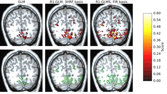
GLM R1-GLM, 3HRF basis R1-GLMS, FIR basis 0.00 0.06 0.12 0.18 0.24 0.30 0.36 0.42 0.48 0.54 0.60 Score
Figure 5: Voxel-wise encoding scores on a single acquisition slice for different estimation methods (first dataset). The metric is Pearson correlation. In the upper column, the voxel-wise score is thresholded at a value of 0.045 (p-value < 0.05), while in the bottom row the 0.055 contour (p-value < 0.001) for the same data is shown as a green line. Despite lacking proper segmentations of visual areas, the estimation methods produce results that highlight meaningful regions of interest around the calcarine fissure. This is particularly visible in the third column where our method R1-GLMS produces results with higher sensitivity than the standard GLM method. In the bottom row it can be seen how the top performing voxels follow well the folding of the gray matter.
GLM with FIR basis GLM with dHRF basis GLMS with FIR basis R1-GLM with FIR basis GLMS with 3HRF basis R1-GLMS with FIR basis GLM with fixed HRF R1-GLMS with 3HRF basis GLMS with fixed HRF R1-GLM with 3HRF basis 0.134 0.148 0.162 * 0.176 0.217 *** 0.227 0.247 * 0.248 0.254 0.276 ** p-value = *< 0.05, **< 10−3, ***< 10−6
Average Decoding Score
R1-GLMS R1-GLM
GLMS GLM
Figure 6: Averaged decoding score for the different method considered (higher is better) on the second dataset. The metric is Kendall tau. Methods that perform constrained HRF estimation significantly outperform methods that use a fixed (reference) HRF. In particular, the best performing method is the R1-GLM with 3HRF basis, followed by the R1-GLMS with 3HRF basis. In underlined typography is the GLM with a fixed HRF which is the method used by default in most software distributions. As in Figure 2, a Wilcoxon signed-rank test is performed and the p-value reported between a given method and the next method in the ordered result list to assess whether the difference in score is significant.
The mean score for the 10 models considered can be seen in Figure 6. Similarly to how we assessed superiority of a given method in encoding, we will say that a given method outperforms another if the paired difference of both scores (this time across folds) is significantly greater than zero. This is computed by performing a Wilcoxon signed rank test across voxels. For this reason we report p-values together with the mean score in Figure 6.
As was the case in encoding, Rank-1 constrained methods obtain the highest scores. In this case however, methods with 3HRF basis outperform methods using FIR basis. This can be explained by factors such as smaller sample size of each of the runs, smaller number of trials in the dataset and experimental design.
5. Discussion
We have compared different HRF modeling techniques and examined their generalization score on two different datasets: one in which the main task was an encoding task and one in which it was a decoding task. We compared 10 different methods that share a common formulation within the context of the General Linear Model. This includes models with canonical and separate designs, with and without HRF estimation constrained by a basis set, and with and without rank-1 constraint. We have focused on voxel-independent models of the HRF, possibly constrained by a basis set, and have omitted for efficiency reasons other possible models such as Bayesian models (Marrelec et al., 2003; Ciuciu et al., 2003; Makni et al., 2005) and regularized methods (Goutte et al., 2000; Casanova et al., 2008).
2012, 2013) that adaptively learn the HRF across several subjects are outside the scope of this work. The latter models are more relevant in the case of standard group studies and second level analysis.
Our first dataset consists of an encoding study and revealed that it is possible to boost the encoding score by appropriately modeling the HRF. We used two different metrics to assess the quality of our estimates. The first metric is the fraction of correctly identified images by an encoding model. For this we computed the activation coefficients on both the training and validation dataset. We then learned a predictive model of the activation coefficients from the stimuli. This was used to identify a novel image from a set of 120 potential images from which the activation coefficients were previously computed. The benefits range from 0.9% points to 8.2% points across R1-constrained methods and subjects. The best-performing model in this task is the R1-GLM with FIR basis. The second metric is the Pearson correlation. By considering the voxel-wise score on a full brain volume we observed that the increase in performance obtained by estimating the HRF was not homogeneous across voxels and more important for voxels that already exhibited a good score with a classical design (GLM) and a fixed HRF. The best-performing method is the Rank-1 with separate designs (R1-GLMS) and FIR basis model, providing a significant improvement over the second best-performing model. We also found substantial variability of the shape in the estimated HRF within a single subject and a single task.
The second dataset consists of a decoding task and the results confirmed that constrained (rank-1) estimation of the HRF also increased the decoding score of a classifier. The metric here is Kendall tau. However, in this case the best performing basis was no longer FIR basis consisting of ten elements but the three elements 3HRF basis (HRF and derivatives) instead, which can be explained by factors such as differences in acquisition parameters, signal-to-noise ratio or by the regions involved in the task.
A higher performance increase was observed when considering the correlation score within the encoding model. This higher sensitivity to a correct (or incorrect) estimation of the HRF can be explained by the fact that the estimation of the HRF is used to generate the BOLD signal on the test set. The metric is the correlation between the generated signal and the BOLD signal. It is thus natural to expect that a correct estimation of the HRF has a higher impact on the results.
In the decoding setup, activation coefficients (beta-map) are computed but the evaluation metric is the accuracy at predicting the stimulus type. The validation metric used for decoding is less sensitive to the HRF estimation procedure than the correlation metric from the encoding study, although it allowed us to observe a statistically significant improvement.
6. Conclusion
We have presented a method for the joint estimation of HRF and activation coefficients within the GLM framework. Based on ideas from previous literature (Makni et al., 2008; Vincent et al., 2010) we assume
the HRF to be equal across conditions but variable across voxels. Unlike previous work, we cast our model as an optimization problem and propose an efficient algorithm based on quasi-Newton methods. We also extend this approach to the setting of GLM with separate designs.
We quantify the improvement in terms of generalization score in both encoding and decoding settings. Our results show that the rank-1 constrained method (R1-GLM and R1-GLMS) outperforms competing methods in both encoding and decoding settings.
AcknowledgementsThis work was supported by grants IRMGroup ANR-10-BLAN-0126-02 and Brain-Pedia ANR-10-JCJC 1408-01. We would like to thank our colleagues Ronald Phlypo and Gael Varoquaux for fruitful discussions.
References
Badillo, S., Varoquaux, G., Ciuciu, P., Jun. 2013a. Hemodynamic Estimation Based on Consensus Clustering. 2013 International Workshop on Pattern Recognition in Neuroimaging, 211–215.
Badillo, S., Vincent, T., Ciuciu, P., Nov. 2013b. Group-level impacts of within- and between-subject hemodynamic variability in fMRI. NeuroImage 82, 433–448.
Bekhti, Y., Zilber, N., Pedregosa, F., Ciuciu, P., Van Wassenhove, V., Gramfort, A., 2014. Decoding perceptual thresholds from MEG/EEG. In: Pattern Recoginition in Neuroimaging (PRNI) (2014). Tubingen, Germany.
Boynton, G. M., Engel, S. A., Glover, G. H., Heeger, D. J., 1996. Linear Systems Analysis of Functional Magnetic Resonance Imaging in Human V1 16 (13), 4207–4221.
Casanova, R., Ryali, S., Serences, J., Yang, L., Kraft, R., Laurienti, P. J., Maldjian, J. a., May 2008. The impact of temporal regularization on estimates of the BOLD hemodynamic response function: a comparative analysis. NeuroImage 40 (4), 1606–18.
Chaari, L., Forbes, F., Vincent, T., Ciuciu, P., Jan. 2012. Hemodynamic-informed parcellation of fMRI data in a joint detection estimation framework. International Conference on Medical Image Computing and Computer-Assisted Intervention 15 (Pt 3), 180–8.
Ciuciu, P., Poline, J.-B., Marrelec, G., Idier, J., Pallier, C., Benali, H., Oct. 2003. Unsupervised robust nonparametric estimation of the hemodynamic response function for any fMRI experiment. IEEE transactions on Medical Imaging 22 (10), 1235–51. Cox, D. D., Savoy, R. L., Jun. 2003. Functional magnetic resonance imaging (fMRI) brain reading: detecting and classifying
distributed patterns of fMRI activity in human visual cortex. NeuroImage 19 (2), 261–270.
Dale, a. M., Jan. 1999. Optimal experimental design for event-related fMRI. Human brain mapping 8 (2-3), 109–14.
Degras, D., Lindquist, M. A., 2014. A hierarchical model for simultaneous detection and estimation in multi-subject fMRI studies. NeuroImage 98C, 61–72.
Doyle, O. M., Ashburner, J., Zelaya, F. O., Williams, S. C. R., Mehta, M. a., Marquand, a. F., Nov. 2013. Multivariate decoding of brain images using ordinal regression. NeuroImage 81, 347–57.
Friston, K. J., Ashburner, J. T., Kiebel, S. J., Nichols, T. E., Penny, W. D., 2011. Statistical parametric mapping: The analysis of functional brain images: The analysis of functional brain images. Academic Press.
Friston, K. J., Holmes, A. P., Poline, J. P., 1995. Statistical parametric maps in functional imaging : A general linear approach. Friston, K. J., Josephs, O., Rees, G., Turner, R., 1998. Nonlinear event-related responses in fMRI. Magnetic Resonance in
Medicine 39 (1), 41–52.
Golub, G. H., Heath, M., Wahba, G., 1979. Generalized cross-validation as a method for choosing a good ridge parameter. Technometrics 21 (2), 215–223.
Goutte, C., Nielsen, F. a., Hansen, L. K., Dec. 2000. Modeling the haemodynamic response in fMRI using smooth FIR filters. IEEE transactions on Medical Imaging 19 (12), 1188–201.
Handwerker, D. a., Ollinger, J. M., D’Esposito, M., Apr. 2004. Variation of BOLD hemodynamic responses across subjects and brain regions and their effects on statistical analyses. NeuroImage 21 (4), 1639–51.
Haynes, J.-D., Rees, G., Jul. 2006. Decoding mental states from brain activity in humans. Nature reviews. Neuroscience 7 (7), 523–34.
Henson, R. N. a., Price, C. J., Rugg, M. D., Turner, R., Friston, K. J., Jan. 2002. Detecting latency differences in event-related BOLD responses: application to words versus nonwords and initial versus repeated face presentations. NeuroImage 15 (1), 83–97.
Horn, R. A., Johnson, C. R., 1991. Topics in matrix analysis. Cambridge university press.
Kay, K. N., Naselaris, Gallant, J. L., 2011. fMRI of human visual areas in response to natural images. CRCNS.org.
Kay, K. N., Naselaris, T., Prenger, R. J., Gallant, J. L., Mar. 2008. Identifying natural images from human brain activity. Nature 452 (7185), 352–5.
Kendall, M. G., 1938. A new measure of rank correlation. Biometrika 30 (1/2), 81–93.
Kriegeskorte, N., Mur, M., Bandettini, P., 2008. Representational similarity analysis–connecting the branches of systems neuroscience. Frontiers in systems neuroscience 2.
Lei, Y., Tong, L., Yan, B., Jan. 2013. A mixed L2 norm regularized HRF estimation method for rapid event-related fMRI experiments. Computational and mathematical methods in medicine 2013, 643129.
Lindquist, M. A., Wager, T. D., 2007. Validity and power in hemodynamic response modeling: A comparison study and a new approach. Hum Brain Mapp 28 (8), 764–784.
Liu, D. C., Nocedal, J., 1989. On the limited memory BFGS method for large scale optimization. Mathematical programming 45 (1-3), 503–528.
Makni, S., Beckmann, C., Smith, S., Woolrich, M., Oct. 2008. Bayesian deconvolution of fMRI data using bilinear dynamical systems. NeuroImage 42 (4), 1381–96.
Makni, S., Ciuciu, P., Idier, J., Poline, J.-B., Sep. 2005. Joint detection-estimation of brain activity in functional MRI: a Multichannel Deconvolution solution. IEEE Transactions on Signal Processing 53 (9), 3488–3502.
Marrelec, G., Benali, H., Ciuciu, P., P´el´egrini-Issac, M., Poline, J.-B., 2003. Robust bayesian estimation of the hemodynamic response function in event-related BOLD fMRI using basic physiological information. Human Brain Mapping 19 (1), 1–17. Miyawaki, Y., Uchida, H., Yamashita, O., Sato, M.-a., Morito, Y., Tanabe, H. C., Sadato, N., Kamitani, Y., Dec. 2008. Visual
image reconstruction from human brain activity using a combination of multiscale local image decoders. Neuron 60 (5), 915–29.
Mour˜ao Miranda, J., Friston, K. J., Brammer, M., May 2007. Dynamic discrimination analysis: a spatial-temporal SVM. NeuroImage 36 (1), 88–99.
Mumford, J. a., Turner, B. O., Ashby, F. G., Poldrack, R. a., Feb. 2012. Deconvolving BOLD activation in event-related designs for multivoxel pattern classification analyses. NeuroImage 59 (3), 2636–43.
Naselaris, T., Kay, K. N., Nishimoto, S., Gallant, J. L., May 2011. Encoding and decoding in fMRI. NeuroImage 56 (2), 400–10. Naselaris, T., Prenger, R. J., Kay, K. N., Oliver, M., Gallant, J. L., 2009. Bayesian reconstruction of natural images from
human brain activity. Neuron 63 (6), 902–915.
Nocedal, J., Wright, S., 2006. Numerical optimization, series in operations research and financial engineering. Springer, New York.
decoding models. Proceedings of the 3nd International Workshop on Pattern Recognition in NeuroImaging (2013), 3–6. Pedregosa, F., Grisel, O., Weiss, R., Passos, A., Brucher, M., 2011. Scikit-learn : Machine learning in python. Journal of
Machine Learning Research 12, 2825–2830.
Poldrack, R. A., Mumford, J. A., Nichols, T. E., 2011. Handbook of Functional MRI Data Analysis. Cambridge University Press.
Poline, J.-B., Brett, M., Aug. 2012. The general linear model and fMRI: does love last forever? NeuroImage 62 (2), 871–80. R¨ohmel, J., Mansmann, U., 1999. Unconditional non-asymptotic one-sided tests for independent binomial proportions when
the interest lies in showing non-inferiority and/or superiority. Biometrical Journal 41 (2), 149–170.
Savitzky, A., Golay, M. J., 1964. Smoothing and differentiation of data by simplified least squares procedures. Analytical chemistry 36 (8), 1627–1639.
Schoenmakers, S., Barth, M., Heskes, T., van Gerven, M., Jul. 2013. Linear reconstruction of perceived images from human brain activity. NeuroImage 83, 951–961.
Tom, S. M., Fox, C. R., Trepel, C., Poldrack, R. a., Jan. 2007. The neural basis of loss aversion in decision-making under risk. Science (New York, N.Y.) 315 (5811), 515–8.
Turner, B. O., Mumford, J. a., Poldrack, R. a., Ashby, F. G., Sep. 2012. Spatiotemporal activity estimation for multivoxel pattern analysis with rapid event-related designs. NeuroImage 62 (3), 1429–38.
Vincent, T., Risser, L., Ciuciu, P., 2010. Spatially adaptive mixture modeling for analysis of fMRI time series. IEEE Transactions on Medical Imaging 29 (4), 1059–1074.
Vu, V. Q., Ravikumar, P., Naselaris, T., Kay, K. N., Gallant, J. L., Yu, B., 2011. Encoding and decoding V1 fMRI responses to natural images with sparse nonparametric models. The annals of applied statistics 5 (2B), 1159.
Wang, J., Zhu, H., Fan, J., Giovanello, K., Lin, W., Jun. 2013. Multiscale adaptive smoothing models for the hemodynamic response function in fMRI. The Annals of Applied Statistics 7 (2), 904–935.
Woolrich, M. W., Behrens, T. E. J., Smith, S. M., Apr. 2004. Constrained linear basis sets for HRF modelling using variational bayes. NeuroImage 21 (4), 1748–61.
Zhang, T., Li, F., Beckes, L., Brown, C., Coan, J. A., Nov. 2012. Nonparametric inference of the hemodynamic response using multi-subject fMRI data. NeuroImage 63 (3), 1754–65.
Zhang, T., Li, F., Beckes, L., Coan, J. a., Jul. 2013. A semi-parametric model of the hemodynamic response for multi-subject fMRI data. NeuroImage 75, 136–45.