an author's https://oatao.univ-toulouse.fr/25978
https://doi.org/10.1016/j.sigpro.2018.05.019
Besson, Olivier An alternative to diagonal loading for implementation of a white noise array gain constrained robust beamformer. (2018) Signal Processing, 152. 79-82. ISSN 0165-1684
increasing distance to the mountains is favoring the presence of mountain waves. We also report on the detection of infrasounds generated by the mountains in the 0.01–0.1 Hz range with a pressure amplitude increase by a factor 2 relative background signal. Besides, we characterized the decrease of microbaroms power when the balloon was flying away from the ocean coast. These observations suggest, in a way similar to microseisms for seismometers, that microbaroms are the main background noise sources recorded in the stratosphere even far from the ocean sources. Finally, we observed a broadband signal above the Andes, between 0.45 and 2 Hz, probably associated with a thunderstorm. The diversity of geophysical phenomena captured in less than a day of observation stresses the interest of high rate pressure sensors on board long-duration balloon missions.
Plain Language Summary
The variations of pressure recorded on board a high-altitude balloon are analyzed to observe various phenomena. When the balloon is passing over the Andes at 33 km altitudes, different waves emitted below it are recorded. Waves produced by storms, atmospheric flows over the mountains, oceanic waves, and thunderstorms are identified in the records. Mountain waves observed by the balloon's instruments are compared to images of the same altitude range obtained by satellites. The poorly documented bass music created by winds in the mountains are observed in certain frequency range, and the sounds created by interfering oceanic waves are slowly decreasing from the coast. The variety of geophysical phenomena observed in less than 1 day demonstrate the power of such missions and instruments. Their interest is extending beyond Earth, because planets with dense atmosphere like Venus can be investigated with such kind of missions.1. Introduction
Propagating waves in the atmosphere induces pressure fluctuations, which can be recorded by sensitive microbarometers. Waves under 20 Hz are divided into two domains: infrasound and gravity waves. Gravity waves are buoyancy-driven and often originate from the deviation of air flow over the large planetary topo-graphic structures (Nappo, 2002; Plougonven et al., 2008), from deep convection and from wind jets (Fritts & Alexander, 2003). Infrasound can be generated by natural or artificial events, such as quakes (Hines, 1960; Lognonné et al., 2016; Martire et al., 2018; Young et al., 2018), nonlinear interactions between ocean waves called microbaroms (Bowman & Lees, 2018; Landès et al., 2014), volcanoes (Assink et al., 2014; Matoza & Fee, 2018), aircraft, or thunderstorms (Lamb et al., 2018). The signals contain the information necessary to better understand and characterize the topography and atmospheric features of a planet and to study its internal structure. In that way, the study of infrasound is directly linked to the planetary and geophys-ical sciences. On Earth, balloon missions represent a great opportunity to study the atmospheric waves over inaccessible regions, such as oceans, mountains, and polar ice caps (Haase et al., 2018). Although
Citation:
Poler, G., Garcia, R. F.,
Bowman, D. C., & Martire, L. (2020). Infrasound and gravity waves over the Andes observed by a pressure sensor on board a stratospheric balloon.
Journal of Geophysical Research: Atmospheres, 125, e2019JD031565.
https://doi.org/10.1029/2019JD031565
Received 27 AUG 2019 Accepted 14 FEB 2020
Accepted article online 10 MAR 2020
Author Contributions
Conceptualization: Raphaël F.
Garcia
Data curation: Daniel C. Bowman,
Léo Martire
Funding Acquisition: Raphaël F.
Garcia
Methodology: Guerman Poler,
Raphaël F. Garcia
Software: Guerman Poler
Validation: Guerman Poler, Daniel C.
Bowman
Writing - Original Draft: Guerman
Poler
Investigation: Guerman Poler,
Raphaël F. Garcia, Léo Martire
Project Administration: Raphaël F.
Garcia
Supervision: Raphaël F. Garcia Writing - review & editing: Raphaël
F. Garcia, Daniel C. Bowman
©2020. American Geophysical Union. All Rights Reserved.
acoustic and gravity waves captured on ground-based sensors have been well studied over several decades (de Groot-Hedlin et al., 2014, 2017; Le Pichon et al., 2010), investigations using high-altitude balloons are more sparse. Infrasound produced by ground explosions was measured by Bowman and Albert (2018), and the issues associated with the stratospheric flight of acoustic arrays are described by Bowman and Lees (2015) and Lees and Bowman (2017). These studies showed that the pressure sensors can be used to observe infrasound and gravity waves. One important reason for this is that, despite lower amplitude signals, pas-sively drifting balloons are less subject to the wind noise and the turbulence, which are the main sources of noise on the ground. However, the low amount of data acquired by those platforms did not allow to quantify yet all the physical phenomena underlying the production and propagation of acoustic and gravity waves. Tests of balloon infrasound sensing technology on Earth is the first step to study other planets on which it is difficult or even impossible to deploy ground stations. Stevenson et al. (2015) studied the feasibility of an infrasound balloon mission on Venus. The Venus ground atmospheric conditions (9e+6 Pa and 700 K) do not allow any long-duration deployment on the surface, even modern technology cannot withstand these temperatures and pressures for more than a couple of hours. In contrast, balloons with infrasound sensors would overpass these limitations and may be able to probe the interior structure of a planet by acoustic pulses from seismic activity on its surface (Garcia et al., 2005) and its atmosphere structure and dynamics (Preston et al., 1986).
Acoustic and gravity waves captured by balloons on Earth and other planets come from a variety of sources. Here, we focus on one point of interest of ULDB (Ultra Long Duration Balloon) mission for which the data have not been analyzed in detail yet: the pass over the Andes. We start by describing the ULDB mission and the associated data, which are used in our analysis (section 2). Then, we will present the various geophysical processes detected when the balloon flew over the Andes and quantify some of the underlying physical phenomena (section 3). Finally, we conclude on the interest of such measurements to characterize wave sources and propagation effects (section 4).
2. Data
2.1. Instrumentation
Our study was based on the analysis of the National Aeronautics and Space Administration's ULDB mis-sion data, described in Bowman and Lees (2018). The balloon was launched from Wanaka, New Zealand, on the 16 May 2016. The batteries of the sensors lasted for 19.5 days, until 6 June 2016. The balloon's total flight duration was 46 days, with an average altitude of 33 km. The balloon had a GPS on board, which provided the longitude, latitude, altitude, and speed of the balloon every 15 min. The microbarometer pay-load was composed of one recording system Omnirecs Datacube, sampled at 200 Hz, and three differential microbarometers InfraBSU. The microbarometer configuration was the following:
• One with positive pressure polarity. • One with negative pressure polarity. • One mechanically disabled.
This setup permits us to distinguish between true pressure signals (polarity reversed between the first two channels, not present on the third channel) with electromagnetic and other interference (common polarity on all three channels). It also allows us to determine the nonpressure noise threshold. The corner frequency of the microphones is not precisely quantified, but since the sensors are at high altitude, it is likely to be very low, around several thousand seconds, which allows us to perform our analysis in the low frequencies domain (Marcillo et al., 2012).
The ULDB data have already been used in Bowman and Lees (2018) to characterize the energy transfer from the microbaroms signal to the thermosphere, which would increase its temperature by several kelvins per day. This flight data was also used to describe the acoustic signature associated with a thunderstorm (Lamb et al., 2018). We focus on a part of the data set that has not been analyzed in detail in order to illustrate the phenomena observed as a balloon crosses a large mountain range. In this configuration, the winds and the balloon are flowing perpendicular to the Andes Mountains ridge in a quasi two-dimensional problem. It represents a perfect situation for the production of topographically driven gravity and acoustic waves. In this manuscript, therefore, we focus on the Andes crossing and downwind phenomena.
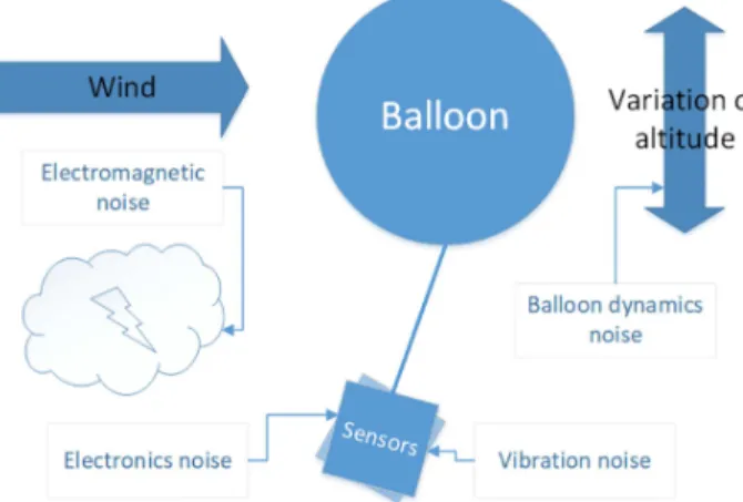
Figure 1. Schematic view of different noise sources sensed by the balloon during the flight. 2.2. Noise Characterization
In order to be able to distinguish between real signals and noise, it is necessary to define and characterize all the noise sources that the balloon may be subject to. The main sources of noise are shown in Figure 1. First, microbarometers are affected by wind noise, one of the main noise sources for the stations at ground level. Electronic noise is intrinsic to the system, and the electromagnetic perturbations come from thunderstorms or auroras. The movement of the balloon and other payloads produces vibrations and the associated noise. In the same way, the balloon is subject to altitude variations; thus, the sensors would not sense the same level of background atmospheric pressure during the whole flight. And eventually, the last noise source is created by acoustic and gravity waves. Therefore, these variations of background pressure need to be characterized, in order to not be mistaken with an atmospheric wave of interest. The noise sources can be summarized by the following equation from Bowman et al. (2018):
𝜖= 𝜖v+ 𝜖e+ 𝜖s+ 𝜖w+ 𝜖p+ 𝜖a, (1)
where different constituents are as follows:
• 𝜖v: stands for sensor motion, that is, vibrations, which is removed from the signal by combination of two channels from active microphones (Bowman & Lees, 2018).
• 𝜖e: corresponds to the outside electromagnetic interference, the associated noise is shown on the signal coming from the mechanically disabled sensor (Bowman & Lees, 2018).
• 𝜖s: depicts the intrinsic sensor electronic noise, which is reduced by using several identical sensors and combining their signal.
• 𝜖w: stands for the wind generated noise. Because the balloon is flying in the stratosphere, at neutral buoy-ancy, thus it experiences near zero differential air flow; hence, the wind noise is negligible (Bowman & Lees, 2016).
• 𝜖p: depicts the nonhydrodystatic pressure fluctuations, which come from the balloon's altitude variations. To estimate its level, we compute the pressure variations sensed by the balloon function of its altitude. • 𝜖a: describes the acoustic and gravity waves pressure signals of interest in this study.
It is important to notice that the mechanically disabled microphone is still slightly sensitive to the spa-tial pressure gradient caused by high-frequency infrasound. Hence, some of the signals recorded on the mechanically disabled microphone can still be caused by pressure waves.
To compute the dynamics noise, we used the GPS altitude measurements and the reanalysis ERA5 (ECMWF, 2018). The high-resolution reanalysis has a spatial resolution of 31 km, a temporal resolution of 1 hr, and a vertical resolution of about 850 m in the 30–35 km altitude range. Once the altitude is acquired, we use the atmospheric model to estimate the associated atmospheric pressure. This conversion is performed through spline interpolation. The GPS measurements are provided every 15 min, so we computed only the low-frequency pressure variations. The sensors are differential barometers; thus, it is impossible to subtract the computed noise from the signal. However, our computation allows us to estimate the power of the noise
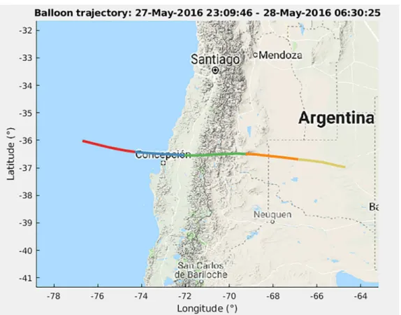
Figure 2. The part of the balloon flight above Andes, which was used for data analysis. The trajectory is divided into
five temporal windows of 1h30 each, distinguishable by the different colors.
coming from the balloon dynamics and to qualify whether the low-frequency recorded signals are impacted by it.
2.3. Methodology
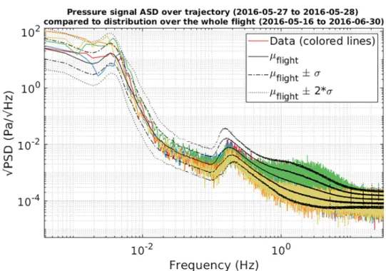
In Figure 2, we present the part of the balloon trajectory which was analyzed in this study. The trajectory is divided into five temporal windows of 1h30 each. The subdivision of the trajectory allows us to correlate the observed signal and the topographic feature over which the balloon is flying. The balloon trajectory starts at 23:00 UTC, or 19:00 local time (LT), on 27 May 2016 and ends at 06:30 UTC (02:30 LT) on 28 May 2016. We conducted the data analysis by studying the amplitude spectral density (ASD, defined as the square root of power spectral density) of the pressure signal on each temporal window. The computed pressure ASD of the balloon trajectory over the Andes is shown in Figure 3. First of all, we estimated the noise coming from balloon dynamics. This noise is a factor 2 to 10 lower than the observed long-period pressure signals; thus, its influence is neglected in our analysis. Second, we observe four different phenomena:
• Activity in the gravity waves domain, under 6 mHz.
• A factor 2 increase in the amplitude of pressure signal just above the mountains between 0.02 and 0.1 Hz compared to other time periods.
• Ocean microbarom signal peaking at 0.01 Pa/√Hz between 0.12 and 0.35 Hz. • Broadband signal between 0.45 and 2 Hz, above the Andes.
In Figure 4, we show the previously computed ASDs, alongside the mean ASD value over the whole flight duration (19.5 days of data acquired mainly above the ocean) with its fluctuation intervals, at one and two standard deviation levels (𝜎 and 2𝜎). To compute these statistical observations, we divided the whole data set on temporal windows of 1h30 duration each and applied the Welch spectral method in the same way as for computation of the Figure 3. From this statistical distribution, computed on more than 300 time windows, we notice that the phenomena described above, especially peaks in the gravity waves domain, mountain infrasound, and thunderstorm signature, are outside the one standard deviation fluctuation interval. Thus,
Figure 3. Pressure signal ASD of the balloon trajectory over the Andes, divided into five temporal windows, which are
shown in Figure 2 with the same colors. The data (solid lines), the sensor noise (dashed lines) estimated from the mechanically disabled sensor, and the balloon dynamics noise (dotted line) are presented. Note the thin 60 Hz line corresponding to contamination by electric networks.
the observed phenomena are probably not due to statistical fluctuations. In the following, we will present each of the detected phenomena and our analysis of associated geophysical processes.
3. Geophysical Processes Detected
3.1. Mountain Gravity Waves
Terrain features such as mountains and valleys can generate gravity waves. This kind of wave plays an impor-tant part in the global circulation by transporting the energy away from the lower atmosphere to the higher levels. These waves have already been observed by stratospheric balloon platforms by using movements of the balloon (Hertzog et al., 2002; Vincent & Hertzog, 2014) and pressure variations (Quinn & Holzworth, 1987). The process behind the generation of these waves is the vertical displacement of the stratified flow when it encounters obstacles. The terrain-generated waves are stationary relative to the ground, because their intrinsic phase speed is equal to the background wind speed, but in opposite direction (Nappo, 2002). The gravity wave domain is separated from the acoustic domain by the Brunt-Väisälä frequency N, which represents the maximum frequency allowed for gravity waves. Above this frequency, the gravity waves are evanescent. Therefore, it is necessary to estimate the value of Brunt-Väisälä frequency at the altitude of the balloon in order to be able to conclude if the observed signal has any physical meaning. We used the formula from (Lighthill, 1978): N2= −g 𝜌 𝜕𝜌 𝜕z− (g c )2 , (2)
where g is the gravity, 𝜌 is the fluid density, z is the altitude, and c the sound speed. Making the assumption that the air is a perfect gas, we obtain this expression:
N2
= (𝛾 −1)(g
c
)2
, (3)
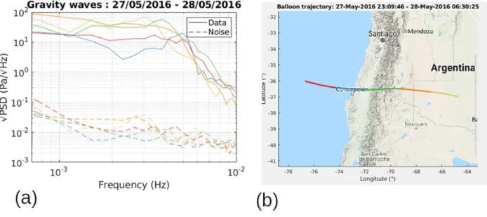
where 𝛾 is the adiabatic index. In order to compute the Brunt-Väisälä frequency at the balloon altitude, we used the ERA5 atmospheric model combined with MSIS-E-90 model (CCMC, 1990). The second model has been used because the atmospheric composition is needed by our codes to compute 𝛾 and additional wave attenuation parameters. Eventually, we computed Brunt-Väisälä angular velocity profile along the balloon trajectory and at the altitude of 33 km, we obtained an average N = 19 mrad/s, corresponding to a frequency of 3.1 mHz. As shown in Figure 5, large signals with a lot of variability are observed in this frequency range and identified as gravity waves.
Figure 4. Pressure signal ASD of balloon trajectory over the Andes (Figure 3) represented with colored lines. ASD
mean value over the whole flight (19.5 days of data mainly acquired above the ocean) 𝜇𝑓lightrepresented with dashed line, and its fluctuation intervals at one standard deviation (𝜎), represented with dash-dotted line, and two standard deviations (2𝜎), represented with dotted line.
In Figure 5, we show the ASD and the temporal signal in the gravity waves spectral domain. First of all, we observe the presence of power peaks, which move from higher frequencies to lower frequencies with the balloon following its trajectory. The observed power peaks start at 4.969 mHz and end at 3.058 mHz. Anderson and Taback (1991) showed that the balloons can resonate at frequencies just below Brunt-Väisälä frequency; thus, the observed power can be partly due to this resonance effect, which is also confirmed by the presence of the peak in this range of frequencies on the mean value over the whole flight, as shown in Figure 4. However, in order to have the resonance, the wave energy must be present; thus, we conclude that we detect gravity waves but the recorded amplitudes do not reflect the real amplitudes of the gravity waves. During the pass over the mountains, the pressure signals in the gravity wave frequency range present a pres-sure signal peak ASD of about 60 Pa/√Hz at 3.9 mHz close to Brunt-Väisälä frequency. Directly after passing the mountains, the power peak disappears (in orange in Figure 5) and reappears in the next temporal win-dow (in yellow in Figure 5), but with a greater peak ASD (85 Pa/√Hz) than that recorded above mountains at a lower frequency (3 mHz) (in green in Figure 5). On the temporal band-pass-filtered signal, we observe the same behavior with 4 Pa amplitudes above mountains, slightly smaller amplitudes directly in the lee of the mountains and once again 4 Pa amplitude in the next time window. However, with the additional hours of data, we note that the amplitudes are decreasing with the distance from the mountains.
The enhanced power just above the mountains (in green in Figures 3–5) could be related to storm activity during the pass of the balloon (see section 3.4). However, the power of pressure signal is increasing again in the lee of the mountain ridge (in yellow in Figures 3–5). This increase is associated to the presence of mountain gravity waves. According to various authors (Ehard et al., 2017; Nappo, 2002; Plougonven et al., 2008), the mountains gravity waves are stationary waves relative to the mountain ridge. When observed in the stratosphere, their wavelengths increase downwind and their amplitudes decrease with the distance from the ridge and with altitude. We compute the associated horizontal wavelengths by using the expression for stationary gravity waves from (Nappo, 2002)
𝜆= 2𝜋u0
Ω , (4)
where u0is the horizontal component of the wind and Ω is the frequency recorded by the balloon sensors.
Figure 5. Gravity waves analysis. (a) The computed ASD over the balloon trajectory, between 0.7 and 10 mHz. (b) The trajectory of the balloon. (c) The
temporal acoustic signal of the studied balloon trajectory with a few hours of additional data, band-pass filtered between 2.294 and 5.734 mHz.
from the ridge. This trend, from smaller wavelengths to larger wavelengths, when following the downwind balloon trajectory is in agreement with the expected behavior of the mountain gravity waves. In addition, the shift of maximum energy relative to the ridge in the downwind direction (Figure 5) can be explained by the upward and downwind propagation of mountain gravity waves (Ehard et al., 2017; Iwasaki et al., 1989). This energy increase cannot be justified by the slight decrease of balloon altitude after the Andes, because only 4% amplitude increase of pressure variations are expected. The hypothesis of detection of mountain
Figure 6. AIRS radiance data (in W·m−2·sr−1· μm−1). (a) Spectrum of AIRS data in the 4.3 μm band taken above the Andes at 13:35 LT (day time) and 01:35 LT
(night time). (b and c) Short wavelength perturbations in AIRS data at 4.3 μm for images acquired respectively at 13:35 LT (day time) and 01:35 LT (night time). Color bar indicates the amplitude of 4.3 μm radiance variations (in W·m−2·sr−1· μm−1). Black line represents the pressure perturbations (band-pass filtered in
the 0.4–2 mHz range) along the balloon's trajectory between 27 May 2016 19:06 GMT (13:06 LT) and 28 June 2016 10:15 GMT (04:15 LT). Red square indicates the balloon position at the time of AIRS data acquisition. The magenta dotted line represents the mean longitude of the Andes.
gravity waves is strengthened by the seasonal observations of high activity in gravity waves domain above Andes from March to October (Hoffmann et al., 2013; Liu et al., 2019).
Besides, we also detected these gravity waves analyzing the Atmospheric Infrared Sounder (AIRS) data (Aumann et al., 2003), shown in Figure 6. AIRS is an instrument on board of the National Aeronautics and Space Administration's Aqua satellite measuring without interruption the midinfrared nadir and sublimb radiance spectra since 2002. To perform our analysis, we used AIRS Level 1B radiance data (NASA, 2009). The data have up to 13 km horizontal resolution. Following the studies of Hoffmann and Alexander (2009), Hoffmann et al. (2013), Sato et al. (2016), and Hoffmann et al. (2016), we selected the data from the 4.3 μm band to sound the stratosphere. Example of spectra in this band are shown in Figure 6. As this band is excited by solar radiation during the day time (non-LTE effect), we observe that the signal is weaker during the night. To obtain the best signal to noise ratio, we only selected the 4.304 and 4.28 μm wavelengths, which are associated with radiance peaks. Then, the obtained image was band-pass filtered; the results are also shown in Figure 6. During the daytime, we observe quite distinguishable gravity waves on the AIRS data, which are much less visible during the nighttime. We also represented the filtered balloon data on the same figure, along the balloon trajectory. The peaks do not match perfectly with the observed gravity waves due to several hours time difference between the two observations. However, the geographical position and the apparent wavelength of the gravity waves from the balloon measurements agree with the AIRS observations.
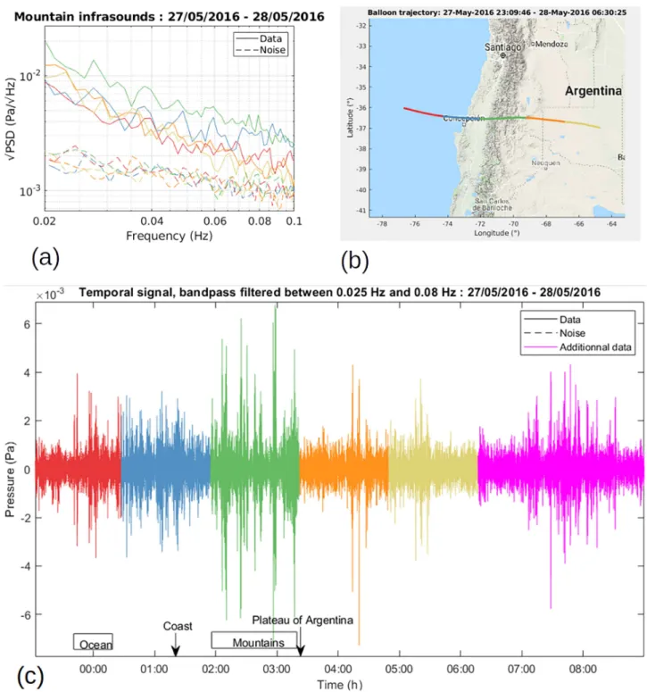
3.2. Infrasounds Generated Over Mountains
Mountain-generated infrasound is still a poorly understood phenomenon; very few theoretical and experi-mental works treat this subject (Bedard, 1978; Chimonas, 1977; Chunchuzov, 1994; Hupe, 2018; Larson et al., 1971). According to these works, the mountains infrasound are probably generated by the wind blowing into the mountain valleys or to turbulence at mountain ridges. The spectral range associated to this phenomenon is between 0.025 and 0.8 Hz. Figure 7 shows that there is a factor 2 increase of pressure signals in this band just above the Andes, evident in both the ASD and on the temporal representation. Our results are in agree-ment with Hupe (2018) that is reporting a significant activity in the same frequency range in this particular region in the May–June time period. This study also suggest that these acoustic waves can be emitted all year long, their detection by ground-based infrasound sensors being limited by varying atmospheric conditions. In addition, the amplitudes of about 2 mPa root-mean-square observed at balloon altitudes in this narrow frequency range (0.025–0.08 Hz) are similar to the ones reported from ground sensors by Hupe (2018) (20 mPa root-mean-square), once the acoustic pressure amplitude decrease between ground and balloon altitude is taken into account (about a factor 10 due to atmospheric density decrease). In addition, due to the low attenuation of these long-period signals in the stratospheric waveguide, peaks of amplitudes observed downstream my be due to the propagation of the acoustic waves generated by the mountains in this direc-tion. This interpretation is reinforced by the apparent periodicity of these signals with about 200 km distance
Figure 7. Infrasound generated by the mountains. (a) The computed ASD over the balloon trajectory, between 20 and 100 mHz. (b) The trajectory of the
balloon. (c) The temporal acoustic signal of the studied balloon trajectory, band-pass filtered between 0.025 and 0.08 Hz.
(Figure 7c), which is approximately the horizontal distance covered by infrasounds reflected in the strato-sphere waveguide. Therefore, we hypothesize that we observed mountain-generated infrasound during this time period.
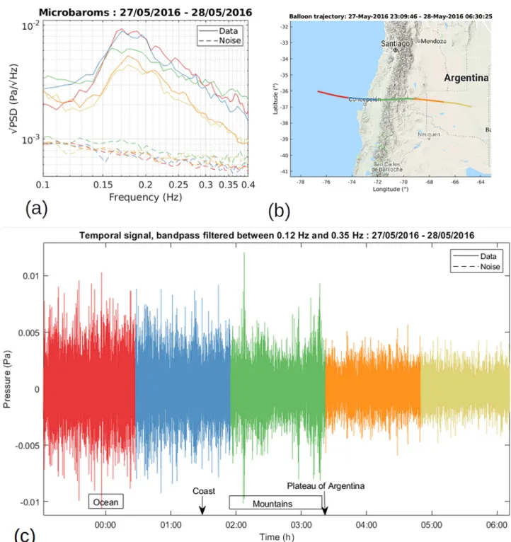
3.3. Ocean Microbarom
The ocean microbarom originates from non linear interactions between ocean waves (Landès et al., 2014). These interactions generate stationary waves, which in turn create acoustic waves in the atmosphere. The
Figure 8. Microbaroms signal. (a) The computed ASD over the balloon trajectory, between 0.1 and 0.4 Hz. (b) The trajectory of the balloon. (c) The temporal
acoustic signal of the studied balloon trajectory, band-pass filtered between 0.12 and 0.35 Hz.
ocean microbarom are the atmospheric equivalent of microseisms (Longuet-Higgins, 1950). The associated spectral range is between 0.12 and 0.35 Hz. The signal is detectable all over the world and consequently is part of acoustic background on Earth. It can be detected on the ground when tropospheric winds are low and stratosphere wind ducts refract them back toward the surface (Campus & Christie, 2009; Bowman & Lees, 2018; Landès et al., 2014).
Figure 8 shows balloon data in the spectral range of microbaroms. The power in this range decreases with increasing distance from the ocean. The decrease is progressive, but the microbaroms peak does not disappear entirely. The same progressive decrease is observed on the temporal signal. A factor 2 difference
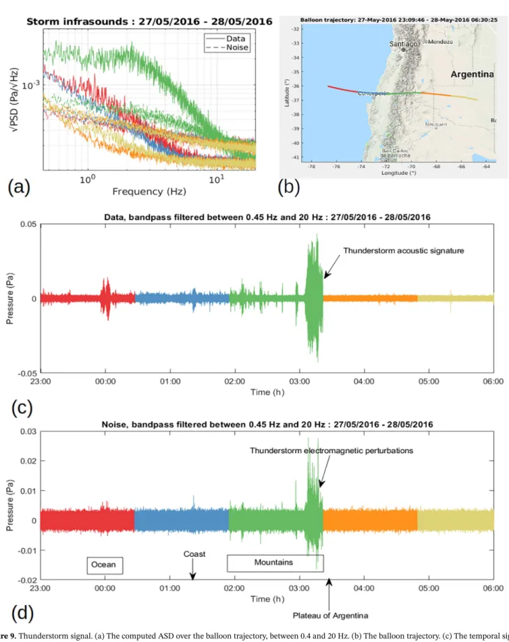
Figure 9. Thunderstorm signal. (a) The computed ASD over the balloon trajectory, between 0.4 and 20 Hz. (b) The balloon trajectory. (c) The temporal signal of
the studied balloon trajectory, band-pass filtered between 0.45 and 20 Hz. (d) Temporal signal of mechanically disabled sensor used to estimate sensor and electromagnetic noises.
of power before and after the mountains is observed. However, this decrease is much less severe than what is predicted by full-wave numerical simulations for direct wave paths: typically a loss factor of ≃10 over ≃70 km distance from the oceanic source (Martire et al., 2018). This observation demonstrates that the ocean micro-barom pressure signals felt by balloon sensors are not only coming from just below the balloon, or along direct paths, but a large part of this signal is due to waves multiply reflected in the stratosphere waveguide. Numerical simulations using GeoAcGlobal software (Blom, 2014), which is using atmospheric attenuation parameters from Sutherland and Bass (2004), in the downstream (i.e., eastern) direction demonstrate that the reflected waves propagate over an horizontal distance of about 180 km and are subject to attenuations of 2 to 6 dB in between each surface reflections. Assuming a continuous and extended oceanic source in the pacific ocean, these simulations predict a decrease of microbarom amplitude of about a factor 1.25 to 2 over 180 km horizontal distance inland. The observed microbarom amplitude decrease of about 3 dB over 200 km (Figure 8c) is consistent with these predictions. As a consequence, our observations demonstrate that microbaroms are propagating in the stratospheric waveguide far from the oceanic sources, in a way similar to microseismic noise propagating globally far from the oceans.
3.4. Thunderstorm Acoustic Signature
Thunderstorms can also generate infrasound. According to Lamb et al. (2018), the acoustic signal of thun-derstorms is only detected in the vicinity of the event. Besides, the thunderstorm has broadband spectral signature between 0.5 Hz and a few hertz. Since the balloon flies above a desert zone, very few meteorologi-cal stations are available. Thus, we did not obtain any precise information on the passage of the storm in this zone. However, using the data provided by the World Wide Lightning Location Network, three thunderbolts were detected in this region before and after the passage of the balloon:
• Date: 27 May 2016 12:23 UTC, Lat: −36.5825◦, Long: −63.915◦
• Date: 28 May 2016 21:27 UTC, Lat: −36.5254◦, Long: −73.3508◦
• Date: 28 May 2016 23:53 UTC, Lat: −36.5254◦, Long: −79.8525◦
The balloon trajectory we analyzed is between 27 May 2016 23:00 UTC and 28 May 2016 06:30 UTC, with a mean latitude of −36.5◦and longitudes between −77◦ and −67◦. The thunderstorm data support the
presence of a storm during these days in the Andes. This is also supported by the presence of clouds and con-vection in the 8.1 μm AIRS data acquired before the balloon passage on 27 May 2016 14:30 LT in this region (not shown). The exact space/time correlation between convective activity and the balloon data cannot be established but all the data sets favor strong convective activity during the passage of the balloon above the Andes.
On the ASD, shown in Figure 9, we observe a broadband signal, between 0.45 and 2 Hz, which corresponds to the thunderstorm signal, as described by Lamb et al. (2018). As shown in Figure 9, the signal is suddenly interrupted in time. It could be explained by the fact that the acoustic signal originating from the storm can be detected only above the storm clouds, directly near to the event. That is why the balloon lost the signal immediately it flew out of the direct vicinity of the thunderstorm clouds. Besides, if we observe the signal of the mechanically disabled sensor, bottom panel of Figure 9, we notice that the acoustic signal comes along with electromagnetic perturbations. These confirm the hypothesis of the storm origin of the signal.
4. Conclusion
Using the ULDB observations, we were able to characterize several infrasound and gravity wave sources as the balloon-borne microbarometers crossed over a large mountain range. We have detected gravity waves above and after the mountain ridge. The waves observed exactly above the Andes are probably due to storms in the troposphere because convective clouds and lightning activity were reported, and thunder-storms acoustic and electromagnetic perturbations are detected by the pressure sensors. However, we expect the increase of pressure signal energy below Brunt-Väisälä frequency after the Andes to be due to the moun-tain gravity waves because it follows frequency shifts (from 4 to 3 mHz) and a decrease of amplitude as a function of distance to the mountain ridge, which are expected for such waves. In addition, we have analyzed the AIRS data, which confirmed the presence of gravity waves in this zone during the passage of the balloon. We have also observed a signal, a factor 2 larger than average background signal in the 0.025–0.08 Hz frequency range, which can be associated with the infrasounds generated by the interactions between the wind and the mountains. Finally, we analyzed the decrease of ocean microbarom power with increasing distance from the coast. Because this decrease is much smaller than the one predicted for direct acoustic
events. Journal of Geophysical Research: Atmospheres, 119, 1140–1153. https://doi.org/10.1002/2013JD021062
Aumann, H. H., Chahine, M. T., Gautier, C., Goldberg, M. D., Kalnay, E., McMillin, L. M., et al. (2003). AIRS/AMSU/HSB on the aqua mission: Design, science objectives, data products, and processing systems. IEEE Transactions on Geoscience and Remote Sensing, 41(2), 253–264.
Bedard, A. J. (1978). Infrasound originating near mountainous regions in Colorado. Journal of Applied Meteorology, 17(7), 1014–1022. Blom, P. S. (2014). GeoAc. https://github.com/LANL-Seismoacoustics/GeoAc
Bowman, D. C., & Albert, S. A. (2018). Acoustic event location and background noise characterization on a free flying infrasound sensor network in the stratosphere. Geophysical Journal International, 213, 1524–1535.
Bowman, D. C., & Lees, J. M. (2015). Infrasound in the middle stratosphere measured with a free-flying acoustic array. Geophysical Research
Letters, 42, 10,010–10,017. https://doi.org/10.1002/2015GL066570
Bowman, D. C., & Lees, J. M. (2016). Direct measurement of the acoustic wave field in the stratosphere. In 2016 IEEE aerospace conference, IEEE.
Bowman, D. C., & Lees, J. M. (2018). Upper atmosphere heating from ocean-generated acoustic wave energy. Geophysical Research Letters,
45, 5144–5150. https://doi.org/10.1029/2018GL077737
Bowman, D., Lees, J., Cutts, J., Komjathy, A., Young, E., Seiffert, K., et al. (2018). Geoacoustic observations on drifting balloon-borne sensors. In A. Le Pichon, E. Blanc, & A. Hauchecorne (Eds.), Infrasound monitoring for atmospheric studies (pp. 125–171). Cham: Springer International Publishing.
CCMC (1990). MSIS model catalogue. https://ccmc.gsfc.nasa.gov/modelweb/, Accessed: 2018-08-15.
Campus, P., & Christie, D. R. (2009). Worldwide observations of infrasonic waves. In A. Le Pichon, E. Blanc, & A. Hauchecorne (Eds.),
Infrasound monitoring for atmospheric studies (pp. 185–234). Netherlands: Springer.
Chimonas, G. (1977). A possible source mechanism for mountain-associated infrasound. Journal of the Atmospheric Sciences, 34(5), 806–811.
Chunchuzov, I. P. (1994). On a possible generation mechanism for nonstationary mountain waves in the atmosphere. Journal of
Atmospheric Sciences, 51(15), 2196–2206.
de Groot-Hedlin, C. D., Hedlin, M. A., Hoffmann, L., Alexander, M. J., & Stephan, C. C. (2017). Relationships between gravity waves observed at Earth's surface and in the stratosphere over the central and eastern United States. Journal of Geophysical Research:
Atmospheres, 122, 11,482–11,498. https://doi.org/10.1002/2017JD027159
de Groot-Hedlin, C. D., Hedlin, M. A. H., & Walker, K. T. (2014). Detection of gravity waves across the USArray: A case study. Earth and
Planetary Science Letters, 402, 346–352.
ECMWF (2018). ERA5 technical documentation. https://confluence.ecmwf.int//display/CKB/ERA5+data+documentation, Accessed: 2018-08-10.
Ehard, B., Kaifler, B., Dörnbrack, A., Preusse, P., Eckermann, S. D., Bramberger, M., et al. (2017). Horizontal propagation of large-amplitude mountain waves into the polar night jet. Journal of Geophysical Research: Atmospheres, 122, 1423–1436. https://doi.org/10.1002/ 2016JD025621
Fritts, D. C., & Alexander, M. J. (2003). Gravity wave dynamics and effects in the middle atmosphere. Reviews of Geophysics, 41(1), 1003. Garcia, R., Lognonné, P., & Bonnin, X. (2005). Detecting atmospheric perturbations produced by Venus quakes. Geophysical Research
Letters, 32, L16205. https://doi.org/10.1029/2005GL023558
Haase, J., Alexander, M, Hertzog, A., Kalnajs, L., Deshler, T., Davis, S., et al. (2018). Around the world in 84 days. EOS, 99. https://doi.org/ 10.1029/2018EO091907
Hertzog, A., Vial, F., DöRnbrack, A., Eckermann, S. D., Knudsen, B. M., & Pommereau, J. P. (2002). In situ observations of gravity waves and comparisons with numerical simulations during the SOLVE/THESEO 2000 campaign. Journal of Geophysical Research, 107(D20), 8292.
Hines, C. O. (1960). Internal atmospheric gravity waves at ionospheric heights. Canadian Journal of Physics, 38, 1441.
Hoffmann, L., & Alexander, M. J. (2009). Retrieval of stratospheric temperatures from atmospheric infrared sounder radiance measure-ments for gravity wave studies. Journal of Geophysical Research, 114, D07105. https://doi.org/10.1029/2008JD011241
Hoffmann, L., Grimsdell, A. W., & Alexander, M. J. (2016). Stratospheric gravity waves at southern hemisphere orographic hotspots: 2003–2014 AIRS/Aqua observations. Atmospheric Chemistry and Physics, 16(14), 9381–9397.
Hoffmann, L., Xue, X., & Alexander, M. J. (2013). A global view of stratospheric gravity wave hotspots located with atmospheric infrared sounder observations. Journal of Geophysical Research: Atmospheres, 118, 416–434. https://doi.org/10.1029/2012JD018658
Hupe, P. (2018). Global infrasound observations and their relation to atmospheric tides and mountain waves (Ph.D. Thesis), Faculty of Physics. https://edoc.ub.uni-muenchen.de/23790/
Iwasaki, T., Yamada, S., & Tada, K. (1989). A parameterization scheme of orographic gravity wave drag with two different vertical partitionings. Journal of the Meteorological Society of Japan. Series II, 67(1), 11–27.
Lamb, O. D., Lees, J. M., & Bowman, D. C. (2018). Detecting lightning infrasound using a high-altitude balloon. Geophysical Research
Letters, 45, 7176–7183. https://doi.org/10.1029/2018GL078401
Aqua NASA mission, and World Wide Lightning Location Network (http:// wwlln.net) for providing the data used in this paper. We also acknowledge three anonymous reviewers for their contributions to the improvement of this scientific paper. This study was funded by “Direction Générale de l'Armement” (French DoD), “Région Occitanie”, and CNES research projects. ULDB data used in our study were retrieved from online repository (https://doi.org/10.5061/dryad. 40877s4). AIRS data were obtained from the AIRS data repository (https:// airs.jpl.nasa.gov/data/get_data). Sandia National Laboratories is a multimission laboratory managed and operated by National Technology & Engineering Solutions of Sandia, LLC, a wholly owned subsidiary of Honeywell International Inc., for the U.S. Department of Energy’s National Nuclear Security Administration under contract DE-NA0003525. This paper describes objective technical results and analysis. Any subjective views or opinions that might be expressed in the paper do not necessarily represent the views of the U.S. Department of Energy or the U.S. Government.
Landès, M., Le Pichon, A., Shapiro, N. M., Hillers, G., & Campillo, M. (2014). Explaining global patterns of microbarom observations with wave action models. Geophysical Journal International, 199(3), 1328–1337.
Larson, R. J., Craine, L. B., Thomas, J. E., & Wilson, C. R. (1971). Correlation of winds and geographic features with production of certain infrasonic signals in the atmosphere. Geophysical Journal, 26(1-4), 201–214.
Le Pichon, A., Blanc, E., & Hauchecorne, A. (2010). Infrasound monitoring for atmospheric studies. Dordrecht, Netherlands: Springer Science & Business Media.
Lees, J. M., & Bowman, D. C. (2017). Balloon borne infrasound platforms: Low noise, high yield. Acoustical Society of America Journal, 141, 4046–4046.
Lighthill, J. (1978). Waves in fluids (pp. 516). Cambridge: Cambridge University Press.
Liu, X., Xu, J., Yue, J., Vadas, S. L., & Becker, E. (2019). Orographic primary and secondary gravity waves in the middle atmosphere from 16-year SABER observations. Geophysical Research Letters, 46, 4512–4522. https://doi.org/10.1029/2019GL082256
Lognonné, P., Karakostas, F., Rolland, L., & Nishikawa, Y. (2016). Modeling of atmospheric-coupled Rayleigh waves on planets with atmosphere: From Earth observation to Mars and Venus perspectives. Acoustical Society of America Journal, 140, 1447–1468. Longuet-Higgins, M. S. (1950). Philosophical Transactions of the Royal Society of London A: Mathematical. Physical and Engineering
Sciences, 243(857), 1–35.
Marcillo, O., Johnson, J. B., & Hart, D. (2012). Implementation, characterization, and evaluation of an inexpensive low-power low-noise infrasound sensor based on a micromachined differential pressure transducer and a mechanical filter. Journal of Atmospheric and
Oceanic Technology, 29(9), 1275–1284.
Martire, L., Brissaud, Q., Lai, V. H., Garcia, R. F., Martin, R., Krishnamoorthy, S., et al. (2018). Numerical simulation of the atmospheric signature of artificial and natural seismic events. Geophysical Research Letters, 45, 12,085–12,093. https://doi.org/10.1029/2018GL080485 Martire, L., Garcia, R., Martin, R., Brissaud, Q., Poler, G., Cadu, A., et al. (2018). Numerical simulations of atmospheric infrasound generated by surface vibrations (ground impact, earthquake, microbaroms), comparison with experimental data. AGU Fall Meeting Abstracts.
Matoza, R. S., & Fee, D. (2018). The inaudible rumble of volcanic eruptions. Acoustics Today, 14, 17–25.
NASA (2009). AIRS technical documentation. https://docserver.gesdisc.eosdis.nasa.gov/repository/Mission/AIRS/3.3_ScienceData ProductDocumentation/3.3.4_ProductGenerationAlgorithms/README.AIRIBRAD.pdf, Accessed: 2018-09-20.
Nappo, C. J. (2002). An introduction to atmospheric gravity waves, International Geophysics (pp. 307). San Diego, CA: Elsevier Science. Plougonven, R., Hertzog, A., & Teitelbaum, H. (2008). Observations and simulations of a large-amplitude mountain wave breaking over
the Antarctic Peninsula. Journal of Geophysical Research, 113, D16113. https://doi.org/10.1029/2007JD009739
Preston, R., Hildebrand, C., Purcell, G., Ellis, J, Stelzried, C., Finley, S., et al. (1986). Determination of venus winds by ground-based radio tracking of the Vega balloons. Science, 231(4744), 1414–1416.
Quinn, E. P., & Holzworth, R. H. (1987). Quasi-Lagrangian measurements of density surface fluctuations and power spectra in the stratosphere. Journal of Geophysical Research, 92(D9), 10,926–10,932.
Sato, K., Tsuchiya, C., Alexander, M. J., & Hoffmann, L. (2016). Climatology and ENSO-related interannual variability of gravity waves in the Southern Hemisphere subtropical stratosphere revealed by high-resolution AIRS observations. Journal of Geophysical Research:
Atmospheres, 121, 7622–7640. https://doi.org/10.1002/2015JD024462
Stevenson, D., Cutts, J. A., Mimoun, D., Arrowsmith, S., Banerdt, W. B., Blom, P., et al. (2015). Probing the interior structure of Venus, Venus Seismology Study Team, Keck Institute for Space Studies.
Sutherland, L. C., & Bass, H. E. (2004). Atmospheric absorption in the atmosphere up to 160 km. The Journal of the Acoustical Society of
America, 115(3), 1012–1032.
Vincent, R. A., & Hertzog, A. (2014). The response of superpressure balloons to gravity wave motions. Atmospheric Measurement
Techniques, 7(4), 1043–1055.
Young, E. F., Bowman, D. C., Lees, J. M., Klein, V., Arrowsmith, S. J., & Ballard, C. (2018). Explosion-generated infrasound recorded on ground and airborne microbarometers at regional distances. Seismological Research Letters, 89(4), 1497–1506.