an author's https://oatao.univ-toulouse.fr/25972
https://doi.org/10.1785/0220180379
van Driel, Martin and Ceylan, Savas and Clinton, John Francis...[et al.] Preparing for InSight: Evaluation of the Blind Test for Martian Seismicity. (2019) Seismological Research Letters, 90 (4). 1518-1534. ISSN 0895-0695
Preparing for InSight: Evaluation of the Blind Test for Martian Seismicity
1Martin van Driel
1, Savas Ceylan
1, John Francis Clinton
2, Domenico Giardini
1, Hector Alemany
12,
2
Amir Allam
19, David Ambrois
12, Julien Balestra
12, Bruce Banerdt
6, Dirk Becker
13, Maren B¨
ose
1,2,
3
Marc S. Boxberg
10, Nienke Brinkman
1, Titus Casademont
13, J´
erˆ
ome Ch`
eze
12, Ingrid Daubar
6, Anne
4
Deschamps
12, Fabian Dethof
13, Manuel Ditz
10, Melanie Drilleau
5, David Essing
13, Fabian Euchner
2,
5
Benjamin Fernando
18, Raphael Garcia
7, Thomas Garth
18, Harriet Godwin
18, Matthew P. Golombek
6,
6
Katharina Grunert
13, Celine Hadziioannou
13, Claudia Haindl
18, Conny Hammer
2, Isabell Hochfeld
13,
7
Kasra Hosseini
18, Hao Hu
14, Sharon Kedar
6, Balthasar Kenda
5, Amir Khan
1, Tabea Kilchling
13,
8
Brigitte Knapmeyer-Endrun
16, 17, Andre Lamert
10, Jiaxuan Li
14, Philippe Lognonn´
e
5, Sarah
9
Mader
13, 20, Lorenz Marten
13, Franziska Mehrkens
13, Diego Mercerat
4, David Mimoun
7, Thomas
10
M¨
oller
10, Naomi Murdoch
7, Paul Neumann
13, Robert Neurath
13, Marcel Paffrath
10, Mark P. Panning
6,
11
Fabrice Peix
12, Ludovic Perrin
8, Lucie Rolland
12, Martin Schimmel
15, Christoph Schr¨
oer
13, Aymeric
12
Spiga
9, Simon Christian St¨
ahler
1, Ren´
e Steinmann
13, Eleonore Stutzmann
15, Alexandre Szenicer
18,
13
Noah Trumpik
13, Maria Tsekhmistrenko
18, C´
edric Twardzik
12, Renee Weber
3, Philipp
14
Werdenbach-Jarklowski
13, Shane Zhang
11, and Yingcai Zheng
1415
1
Institute of Geophysics, ETH Z¨
urich Sonneggstrasse 5, 8092 Z¨
urich, Switzerland
16
2
Swiss Seismological Service, ETH Z¨
urich Sonneggstrasse 5, 8092 Z¨
urich, Switzerland
17
3
NASA Marshall Space Flight Center, ST13/NSSTC 2047, Huntsville, Alabama 35805 U.S.A.
18
4
CEREMA M´
editerran´
ee, project team MOUVGS, 500 route des Lucioles, 06903, Sophia Antipolis,
19
France
20
5
Institut de Physique du Globe de Paris, Sorbonne Paris Cit´
e, Universit´
e Paris Diderot, 75013 Paris,
21
France
22
6
Jet Propulsion Laboratory, California Institute of Technology Pasadena, California 91109 U.S.A.
23
7
ISAE-SUPAERO, Universit´
e de Toulouse, DEOS/ SSPA, 10 av E. Belin, 31400 Toulouse, France
24
8
Centre National d’Etudes Spatiales, 18 Avenue Edouard Belin, 31400 Toulouse, France
25
9
Laboratoire de M´
et´
eorologie Dynamique (LMD/IPSL), Sorbonne Universit´
e, Centre National de la
26
Recherche Scientifique, ´
Ecole Polytechnique, ´
Ecole Normale Sup´
erieure, Paris, France
27
10
Ruhr University Bochum, Faculty of Geosciences, Institute of Geology, Mineralogy and Geophysics,
28
44780 Bochum, Germany
29
11
Department of Physics, University of Colorado Boulder, Boulder, Colorado 80309, U.S.A.
30
12
Universit´
e Cˆ
ote d’Azur, Observatoire de la Cˆ
ote d’Azur, CNRS, IRD, G´
eoazur, France
31
13
Institute of Geophysics, University of Hamburg, Bundesstrasse 55, 20146 Hamburg, Germany
32
14
Department of Earth and Atmospheric Sciences, University of Houston, Houston, Texas, U.S.A.
33
15
Institut de Physique du Globe de Paris, 1 rue Jussieu, 75252 Paris, Cedex 5, France
34
16
Max-Planck-Institut f¨
ur Sonnensystemforschung, Justus-von-Liebig-Weg 3, 37077 G¨
ottingen,
35
Germany
36
17
now at: Institute of Geology and Mineralogy, University of Cologne, Vinzenz-Pallotti-Str. 26, 51429
37
Bergisch Gladbach, Germany
38
18
Department of Earth Sciences, University of Oxford, South Parks Road, Oxford OX1 3AN, UK
39
19
Department of Geology & Geophysics, University of Utah, Salt Lake City, Utah, U.S.A.
40
20
Karlsruhe Institute of Technology (KIT), Geophysical Institute, Hertzstr. 16, 76187 Karlsruhe,
41
Germany
42
April 15, 2019
Abstract
44In December 2018, the NASA InSight mission deployed a seismometer on the surface of Mars. In preparation for the 45
data analysis, in July 2017 the Mars Quake Service initiated a blind test, in which participants were asked to detect and 46
characterize seismicity embedded in a one Earth year long synthetic dataset of continuous waveforms. Synthetic data were 47
computed for a single station, mimicking the streams that will be available from InSight as well as the expected tectonic 48
and impact seismicity, and noise conditions on Mars (Clinton et al. 2017). In total, 84 teams from 20 countries registered 49
for the blind test and 11 of them submitted their results in early 2018. The collection of documentations, methods, ideas 50
and codes submitted by the participants exceeds 100 pages. The teams proposed well established as well as novel methods 51
to tackle the challenging target of building a global seismicity catalogue using a single station. This paper summarizes 52
the performance of the teams, and highlights the most successful contributions. 53
Introduction
54The National Aeronautics and Space Administration (NASA) discovery-class mission InSight (Interior exploration using 55
Seismic Investigations, Geodesy and Heat Transport, Banerdt et al. 2013, http://insight.jpl.nasa.gov) to Mars was 56
launched on May 5th, 2018 and landed successfully on November 26th. It is dedicated to determining the constitution 57
and interior structure of Mars. For this purpose, InSight deployed a single seismic station with both broadband and 58
short-period seismometers on the surface of Mars, together with a number of other geophysical (Folkner et al. 2018; Spohn 59
et al. 2018) and meteorological (Spiga et al. 2018) sensors. The seismic instrument package (SEIS) is specifically designed 60
for martian conditions to record marsquakes as well as meteoroid impacts, and transmit data back to Earth for analysis 61
(Lognonn´e et al. 2019, www.seis-insight.eu).
62
The Marsquake Service (MQS, Clinton et al. 2018) is tasked with the prompt review, detection and location of all 63
martian seismicity recorded by InSight. It will also manage the seismicity catalogue, refining locations using the best 64
available Mars models as they are developed during the project. To prepare the InSight science team and the wider 65
seismological community for the data return, the MQS sent an open invitation to participate in a blind test to detect and 66
locate seismic events hidden in a synthetic data set, which was published in SRL in July 2017 (Clinton et al. 2017). The 67
data set was made available at http://blindtest.mars.ethz.ch/ in August 2017 with mandatory registration. Following 68
the submission deadline in February 2018, the true model and event catalogue together with the original waveform data 69
are now openly available online. 70
Purpose of the Test
71
The blind test was initiated with the main purpose of improving and extending the set of methods for event location, 72
discrimination and magnitude estimation as well as phase identification and source inversion to be applied in routine 73
analysis of the InSight data set by collecting ideas from outside the InSight science team. It also helped to raise the profile 74
of the InSight mission and to familiarize interested scientists with the data set to be expected from Mars. 75
Beyond this, the test also initiated a major effort to generate a single, consistent, temporal, synthetic data set that 76
collected all best pre-landing estimates of seismicity, impacts, synthetic seismograms, atmospheric pressure variations and 77
related noise, instrument self-noise and 1D structure models. The data set was made available in the same formats, and 78
using similar web services as are now available for the real data from Mars. For this reason, the data set was also used 79
for various operational readiness tests as well as scientific testing purposes in preparation for data return. 80
Furthermore, the submitted catalogues allow to derive detection and location thresholds as a function of magnitude and 81
distance, that are not based on simple signal to noise ratio assumptions, but include the whole complexity of identifying 82
and locating events in the time series. It is important to note though, that this data set included randomly distributed 83
events over the sphere. Compared to the global fault distribution (Knapmeyer et al. 2006), this model may have too 84
many events near the landing site, so the total number of detectable events in this dataset may be higher than predicted 85
by recent seismicity models of similar total activity (Plesa et al. 2018). This needs to be accounted for if the detection 86
threshold determined in this test is used for constraining seismic activity rates. 87
In the invitation, we envisioned a quantitative scoring in different categories (event detection and localization accuracy 88
in different magnitude classes, impact discrimination and focal mechanism), but this turned not to be feasible given the 89
heterogeneity of the submissions and relatively small number of detectable events in the data. Instead, we decided to 90
focus on visual comparisons of the performances and compare them to the level 1 (L1) requirements of the mission, i.e. 91
the required accuracy to achieve InSight’s science objectives. The L1 requirements for quake location are 25% in distance 92
and 20 degrees in azimuth (Banerdt et al. 2013). 93
Overview of the Test Data Set
94
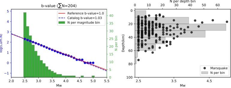
The event catalogue included a total of 204 tectonic marsquakes as well as 36 impacts (Fig. 1), with only a fraction of 95
them producing seismic signals above the noise level. The events were randomly distributed over the whole planet where 96
the depth distribution of tectonic events followed a skewed Gaussian distribution with a maximum allowed depth of 80 97
km. The maximum event size was Mw= 5 and the magnitude-frequency distribution approximates a Gutenberg-Richter
98
distribution with a = 4.88, b = 1; events with Mw< 2.5 were neglected (see Fig. 2 and Ceylan et al. 2017).
99
The impact catalogue is based on Teanby (2015) and the size distribution of observed newly dated craters (Daubar 100
et al. 2018), again assuming a globally random distribution. To restrict amplitudes to levels similar to Mw2.5 events, we
101
only include impacts with impactor mass larger than 100 kg and assume an impact velocity of 10 km/s. 102
The seismic signals were computed using AxiSEM (Nissen-Meyer et al. 2014) and Instaseis (van Driel et al. 2015) as 103
solutions to the elastic-wave equation in radially symmetric planet models. Continuous time series were then created by 104
superimposing the event based data with seismic noise that reflects the pre-landing estimates for the surface installed 105
instruments at the landing site (Murdoch et al. 2017a; Murdoch et al. 2017b; Mimoun et al. 2017; Kenda et al. 2017). It 106
includes noise generated by the sensors and systems themselves, as well as through sources in martian environment (such 107
as fluctuating pressure-induced ground deformation, the magnetic field, and temperature-related noise) and nearby lander 108
(such as wind-induced solar panel vibrations). 109
Synthetic data were generated from one of the 14 candidate models (Zharkov and Gudkova 2005; Rivoldini et al. 2011; 110
Khan et al. 2016) which were published as part of the data set, but the model choice was not revealed to participants. 111
The model used for creation of waveform data set is shown in Figure 3 which explains two prominent features observed 112
by most participating teams: 1) Clear S-wave arrivals were absent in most events due to the low velocity region in the 113
upper mantle, which made distance estimations based only on relative P and S travel times very difficult, and 2) at the 114
same time, the bedrock layer at the surface acted as a wave guide and caused a prominent P-coda arrival, that could be 115
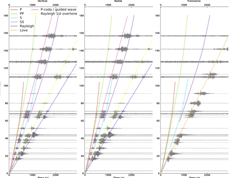
used for estimating locations in this 1D setting (see Fig. 4 for an overview of the most visible events). Such a phase is 116
observed over long distances in specific settings on Earth, such as oceanic crust of constant thickness (e.g. Kennett and 117
Furumura 2013), but in this blind test, it should be considered an artifact from the simple 1D model. It is not expected 118
to be observed as a global phenomenon on Mars due to attenuation from 3D scattering. 119
An overview of responsibilities for the generation of the data set can be found in Table 1; further details can be found 120
in Clinton et al. (2017). Based on the experience gained and performance of the MQS in particular within this test, the 121
MQS is currently refining the location strategies and running an ORT (operational readiness test) with synthetic data 122
computed in a 3D model. 123
In the following sections, we first summarize the methods used by each team. Then, we compare the success of each 124
submission in terms of event detection, as well as estimated event distance, back-azimuth and origin time against the true 125
event parameters. 126
Participation and Methods
127In order to ensure effective communication with participants or anyone who wanted to experiment, registration for the 128
test was mandatory for accessing the dataset. On the other hand, participation was completely voluntary; but we strongly 129
encouraged all registrants to submit their results, particularly with event catalogues. In total, 84 teams registered and 11 130
of them submitted their analysis. Due to the lack of feedback, we do not have a further overview on how test data was 131
used by other teams that downloaded the data but chose not to participate. 132
The participating teams were composed of researchers both from inside (IPGP, MQS, Max Planck) and outside (Col-133
orado, Geoazur, Houston, Utah) the InSight science team. Participant profiles were rather diverse including senior
134
researchers as well as PhD (Bochum, Oxford), masters (Hamburg) and even high school students (SEISonMars@school). 135
See Table 2 for a list of the teams and their members. In Table 3, we summarize the wealth of methods used by the 136
participants with references to previous publications as much as possible, but a significant fraction of the methods applied 137
by participants appears to have been developed specifically for this test. 138
Most teams inspected the waveforms visually or used spectrograms for event detection, while four teams (Bochum, 139
Geoazur, Hamburg, Utah) also utilized STA/LTA algorithms with manual review for this purpose. In the case of a 140
single station, event distance can be estimated using relative travel times between different body- and surface waves, 141
and multi-orbit surface waves for the larger events. While the latter is independent of the model (Panning et al. 2017), 142
body and minor arc surface wave travel times need a reference model for distance estimation. Hence, most teams tried 143
to first determine the model from the 14 candidate models and then computed locations for that model. Three teams 144
(Bochum, Colorado, MQS), however, used probabilistic methods to account for the inherent trade off between model 145
and distance. Combining the distance estimate with the back-azimuths of the event and the known station location, 146
an absolute location can be derived. The participants used a large variety of both P and Rayleigh polarization analysis 147
methods for this purpose. Only two teams (Houston and MQS) attempted to determine depth, which was difficult as most 148
events did not show clear depth-phases. 149
Only one team (Colorado) attempted to decorrelate the atmospheric pressure signals to reduce the noise; and one other 150
team (Hamburg) classified pressure events automatically, while others relied on a visual check to exclude those from the 151
catalogue. The Houston team was the only group to derive surface wave phase velocities. Two teams did not submit a 152
catalogue but applied methods that facilitate event detection and phase recognition: IPGP focused on crustal structure 153
and polarization analysis rather than event locations and Max Planck implemented an HMM (Hidden Markov Models) 154
approach to detect events, which allowed them to provide only event detection times and no origin times. 155
None of the teams submitted information on the focal mechanisms within this test, but the method of St¨ahler and
156
Sigloch (2014) has been applied successfully after the submission deadline by the MQS team for the largest 3 events 157
(Clinton et al. 2018). 158
Performance
159In the blind test announcement (Clinton et al. 2017), it was stated that it was mandatory to provide a location and 160
origin time. A number of teams were only able to provide approximate detection times without locations and others only 161
provided locations for parts of their catalogue. We decided to also show these results, though we understand that other 162
teams that closely followed this rule may have left out detected events that they were not able to locate and hence the 163
detection statistics needs to be interpreted with care. 164
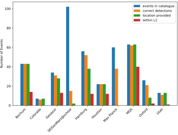
Figure 5 gives an overview of the performance by different teams in detecting and locating events: 165
• The blue bars represent the total number of events in each catalogue, that besides true and false detections, may also 166
include multiple detections for a single event. This was in particular the case for the fully automatic Hidden Markov 167
Model (HMM) approach from the Max Planck team, since HMM is fundamentally a pattern matching approach 168
operating on certain statistics that heavily relies on proper classification and representation of training events. In 169
this application, only a single training event was used. 170
• The orange bars represent the number of events that could be associated with an event in the true catalogue solely 171
based on the origin time and with duplicate detections removed. As we prevented event waveforms from overlapping 172
in the seismicity catalogue, the association is straightforward. We assume any event time submitted that occurs 173
within a window from 750 seconds before and 1500 seconds after the true origin time as correct. The three teams 174
that performed best in detection (MQS, Hamburg, Bochum) all relied on a high degree of visual data inspection, 175
while two of them (Hamburg, Bochum) assisted by STA/LTA triggering. Comparing seismic and pressure data 176
visually allowed these teams to exclude most non-seismic events. MQS produced daily spectrograms that were 177
visually scanned by different members of the team, which proved a very effective way to maximize event detection. 178
• The green bars represent the number of events for which full location information was provided (origin time, distance 179
and azimuth). 180
• Finally, the red bars represents events that were located within the InSight mission L1 requirements for location 181
accuracy. 182
Figure 6 shows a more detailed view of the 10 submitted catalogues, highlighting false detections (blue vertical lines) as 183
well as detection and location of quakes (circles) impacts (star symbols). The rate of correct detection and location as well 184
as false detections varies significantly over the time span of the dataset. This may be related to sharing of the workload 185
between multiple operators; for example MQS split the initial detection on a monthly bases between team members. 186
In the following, we focus on the six teams that provided the most complete results in terms of the number of events 187
correctly located within L1 requirements: Bochum, Geoazur, Hamburg, Houston, MQS and Oxford. MQS submitted two 188
catalogues (focusing on absolute and relative distances, respectively), but as they are of very similar quality and were 189
built iteratively using information from both approaches, we treat them as one for the purpose of this paper. 190
Distance Magnitude Trade-off
191
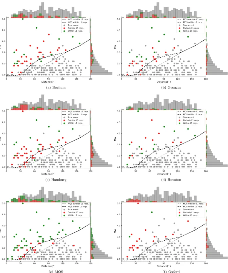
Figure 7 provides an overview of the six most complete catalogues with respect to distance and magnitude. It also reveals 192
that although MQS had the highest number of correct detections, a handful of events were missed that other teams were 193
able to detect, and some detected events were located more precisely by other teams. MQS carefully analyzed each of 194
these events again to identify the root cause of these mislocations and unidentified events. Besides mislabeled seismic 195
phases, several issues in the MQS workflow were recognized and resolved, with the most important improvement being 196
the increase of the overlap in the daily plots used for visual screening. 197
Most of the six teams detected all events above magnitude 4, globally. Between magnitude 3 and 4, several teams 198
detected all events until approximately 40 degree distance, even though they could not locate them within the L1 require-199
ments. MQS detected all events above magnitude 3.5 and all events above magnitude 2.5 within 30 degree distance, which 200
suggests that the detection threshold may be even lower than 2.5 for regional events. The detection curve for MQS is only 201
distance/magnitude dependent, without an indication of an effect of different focal mechanisms. 202
Distance Estimation
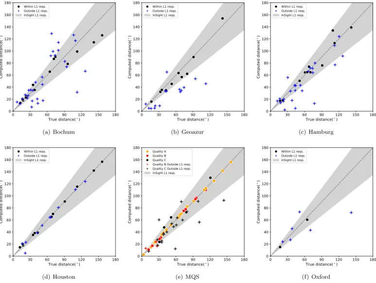
203
Distance estimation (Fig. 8) was complicated by the low velocity layers in the upper mantle, which made S-waves very 204
hard to identify in the data with the given noise. An easy estimate based only on the traveltime difference between P and 205
S phase could hence not be applied to most events. On the other hand, Rayleigh wave group arrival times could be used 206
with unrealistically high accuracy in this 1D model, which is one reason for running the current ORT with 3D synthetics. 207
This new test suggests that including estimates of crustal thickness variations from gravity (Wieczorek and Zuber 2004), 208
topography from MOLA (Mars Orbiting Laser Altimeter), and ellipticity lateral variations of surface wave arrival times 209
of up to a few hundred seconds should be expected. 210
An additional simplification was employed by most teams by determining the correct model from the 14 candidate 211
models based on the biggest event in the dataset (see table 3) and then using that model to locate the smaller events. In 212
practice, a number of small events are expected to be seen in the data before any event that is big enough to constrain 213
the model. To add this complexity to the problem, the data in the new 3D test was released in weekly chunks. 214
The MQS catalogue included a data quality classification, where reliable locations where classified as quality A, 215
unreliable locations as quality B, and very unreliable/unconstrained locations as quality C. This figure indicates that only 216
class C and a few class B events could not be located correctly (Clinton et al. 2018). 217
Back-Azimuth Estimation
218
The back-azimuth estimation in Figure 9 reveals that some methods suffer from a 180◦ ambiguity, which can however
219
be resolved by either assuming retrograde Rayleigh motion or including the incidence angle in P-wave azimuth estimates 220
(Panning et al. 2015; B¨ose et al. 2016). Like for the distance estimate, all MQS quality A and the majority of quality B
221
location estimates meet the L1 requirement. 222
Origin Time Estimation
223
The error in origin time estimation is closely related to distance estimation by the fixed model set that was provided for 224
this test, and this can also be observed in the strong correlation in performance for distance and origin time (Fig. 10). 225
Similar arguments as in the distance estimation apply for the model complexities and 3D effects. 226
Impact Discrimination
227
Only one team (MQS) classified the event type as quake/impact in their catalogue. Only a single event was identified as 228
an impact, which was correct, and no other event was mis-labeled as impact. MQS did miss the biggest impact event of 229
the dataset in the detection stage. Hence we cannot evaluate the distinction capability in this test and just document 230
the three strongest impact events together with three quakes for reference in Figure 11: If the signal is above the noise, 231
the waveforms appear very distinct from quakes due to trapped energy in the high Q shallow layers of the 1D model as 232
well as very short period surface waves excited by the surface source. In contrast, quakes at depth neither excite trapped 233
waves in the shallow layers in this 1D model due to Snel’s law nor the very short period surface waves due to their limited 234
penetration depth. 235
MQS’ classification of the impact was purely based on the waveform’s appearance, which they recognised as very 236
different from all other events. With very few impact events ever seismically recorded and the distinct impact behaviour 237
due to the atmosphere on Earth compared to the Moon, there is no well established discrimination technique. Gudkova 238
et al. (2011) suggest a different spectral content of impacts compared to quakes for the Moon. Other criteria include the 239
depth of the event, although the absence of depth phases is difficult to demonstrate. Additionally, newly detected craters 240
on satellite images from Mars might help to discriminate impact events if they can be correlated in time and location. 241
Conclusions
242The submissions to this blind-test have provided the InSight science team with a range of new ideas and brought the 243
specific challenges of single station seismology on Mars to a broader range of seismologists from the general community. 244
In practice, the main benefits of the test to the MQS was that it provided the opportunity to thoroughly test software 245
and routines as well as benchmark the event detection and location capabilities on a previously unavailable quality data 246
set; and to evaluate whether there are new or existing methodologies that were overlooked and could significantly improve 247
MQS’ performance. 248
Finally, various teams contributed to this 1D test with a number of useful and different ideas; however, the algorithms 249
established in MQS produced comparable or better performance. Further evaluation in the light of the 3D effects from 250
synthetics as well as the actual seismicity observed by the InSight seismometers will be necessary to decide if MQS will 251
adopt any of the suggested methods from other teams. From the test it is also obvious that the best performances were 252
produced by the teams that had the time to dedicate to the test – an important lesson for MQS for organizing routine 253
operations: one team member is always on duty to analyze all new data for possible seismic events with another person 254
as backup. Any suspected event is then analyzed carefully by the review team before communicating to the whole science 255
team (see Clinton et al. 2018, for details on the operations). 256
The blind test experience has helped forming the basis for the currently running operational readiness tests with 3D 257
synthetic data for both the MQS and MSS (Mars Structure Service Panning et al. 2017), which give an opportunity to 258
the operational teams to train daily data review. 259
Data and Resources
260The test data set is described in more detail by Clinton et al. (2017) and available online at http://blindtest.mars. 261
ethz.ch/ (last accessed December 2018). Figures are created using ObsPy (Krischer et al. 2015). Submissions (catalogues 262
and documentation) by individual teams are not publicly available. 263
Acknowledgements
264The co-author list of this paper includes contributors to the evaluation (up to and including D. Giardini), contributors to 265
the data set and invitation paper (Table 1) as well as the participants of the blind test (Table 2). 266
This work was jointly funded by (1) Swiss National Science Foundation and French Agence Nationale de la Recherche 267
(SNF-ANR project 157133 “Seismology on Mars”), (2) Swiss State Secretariat for Education, Research and Innovation 268
(project “MarsQuake Service—Preparatory Phase”) and (3) ETH Zurich (project “Preparatory phase for Mars InSight 269
Ground Segment Support”). Additional support came from the Swiss National Supercomputing Centre (CSCS) under 270
project ID s682. Some of the research described in this article was supported by the InSight (Interior exploration using 271
Seismic Investigations, Geodesy and Heat Transport) project, Jet Propulsion Laboratory, California Institute of Technol-272
ogy, under a contract with the National Aeronautics and Space Administration (NASA). The Houston team was partially 273
funded by EAR-1621878. A. Spiga and L. Rolland acknowledge funding by CNES (Centre National d’ ´Etudes Spatiales).
274
This paper constitutes InSight Contribution Number 93. 275
References
276Allam, A. A., Y. Ben-Zion, and Z. Peng (2014). Seismic Imaging of a Bimaterial Interface Along the Hayward Fault, CA, 277
with Fault Zone Head Waves and Direct P Arrivals, Pure Appl. Geophys. 171.11 2993–3011. 278
Allam, A. A., V. Schulte-Pelkum, Y. Ben-Zion, C. Tape, N. Ruppert, and Z. E. Ross (2017). Ten kilometer vertical Moho 279
offset and shallow velocity contrast along the Denali fault zone from double-difference tomography, receiver functions, 280
and fault zone head waves, Tectonophysics 721 56–69. 281
Banerdt, W. B., S. Smrekar, P. Lognonn´e, T. Spohn, S. Asmar, D. Banfield, L. Boschi, U. Christensen, V. Dehant, W. M.
282
Folkner, D. Giardini, W. Goetze, M. P. Golombek, M. Grott, T. Hudson, C. Johnson, G. Kargl, N. Kobayashi, J. Maki, 283
D. Mimoun, A. Mocquet, P. Morgan, M. P. Panning, W. Pike, J. Tromp, T. van Zoest, R. Weber, M. A. Wieczorek, 284
R. F. Garcia, and K. Hurst (2013). InSight: A Discovery Mission to Explore the Interior of Mars, 44th Lunar Planet. 285
Sci. Conf. 1915. 286
Bayer, B., R. Kind, M. Hoffmann, X. Yuan, and T. Meier (2012). Tracking unilateral earthquake rupture by P-wave 287
polarization analysis, Geophys. J. Int. 188.3 1141–1153. 288
B¨ose, M., J. F. Clinton, S. Ceylan, F. Euchner, M. van Driel, A. Khan, D. Giardini, P. Lognonn´e, and W. B. Banerdt
289
(2016). A Probabilistic Framework for Single-Station Location of Seismicity on Earth and Mars, Phys. Earth Planet. 290
Inter. 262 48–65. 291
B¨ose, M., D. Giardini, S. St¨ahler, S. Ceylan, J. F. Clinton, M. van Driel, A. Khan, F. Euchner, P. Lognonn´e, and W. B.
292
Banerdt (2018). Magnitude Scales for Marsquakes, Bull. Seismol. Soc. Am. 108.5A 2764–2777. 293
Ceylan, S., M. van Driel, F. Euchner, A. Khan, J. F. Clinton, L. Krischer, M. B¨ose, S. C. St¨ahler, and D. Giardini (2017).
294
From Initial Models of Seismicity, Structure and Noise to Synthetic Seismograms for Mars, Space Sci. Rev. 211.1-4 295
595–610. 296
Clinton, J., D. Giardini, M. B¨ose, S. Ceylan, M. van Driel, F. Euchner, R. F. Garcia, S. Kedar, A. Khan, S. C. St¨ahler, B.
297
Banerdt, P. Lognonne, E. Beucler, I. Daubar, M. Drilleau, M. Golombek, T. Kawamura, M. Knapmeyer, B. Knapmeyer-298
Endrun, D. Mimoun, A. Mocquet, M. Panning, C. Perrin, and N. A. Teanby (2018). The Marsquake Service: Securing 299
Daily Analysis of SEIS Data and Building the Martian Seismicity Catalogue for InSight, Space Sci. Rev. 214.8. 300
Clinton, J., D. Giardini, P. Lognonn´e, B. W. Banerdt, M. van Driel, M. Drilleau, N. Murdoch, M. P. Panning, R. Garcia,
301
D. Mimoun, M. Golombek, J. Tromp, R. Weber, M. B¨ose, S. Ceylan, I. Daubar, B. Kenda, A. Khan, L. Perrin, and
302
A. Spiga (2017). Preparing for InSight: An Invitation to Participate in a Blind Test for Martian Seismicity, Seismol. 303
Res. Lett. 88.5 1290–1302. 304
Daubar, I., P. Lognonn´e, N. A. Teanby, K. Miljkovic, J. Stevanovi´c, J. Vaubaillon, B. Kenda, T. Kawamura, J. Clinton, A.
305
Lucas, M. Drilleau, C. Yana, G. S. Collins, D. Banfield, M. Golombek, S. Kedar, N. Schmerr, R. Garcia, S. Rodriguez, 306
T. Gudkova, S. May, M. Banks, J. Maki, E. Sansom, F. Karakostas, M. Panning, N. Fuji, J. Wookey, M. van Driel, 307
M. Lemmon, V. Ansan, M. B¨ose, S. St¨ahler, H. Kanamori, J. Richardson, S. Smrekar, and W. B. Banerdt (2018).
308
Impact-Seismic Investigations of the InSight Mission, Space Sci. Rev. 214.8. 309
Eisermann, A. S., A. Ziv, and G. H. Wust-Bloch (2015). Real-Time Back Azimuth for Earthquake Early Warning, Bull. 310
Seismol. Soc. Am. 105.4 2274–2285. 311
Fernando, B., M. Tsekhmistrenko, and K. Hosseini (2018). Training martian seismologists for InSight, Astron. Geophys. 312
59.5 5.17–5.21. 313
Folkner, W. M., V. Dehant, S. Le Maistre, M. Yseboodt, A. Rivoldini, T. Van Hoolst, S. W. Asmar, and M. P. Golombek 314
(2018). The Rotation and Interior Structure Experiment on the InSight Mission to Mars, Space Sci. Rev. 214.5. 315
Gudkova, T. V., P. Lognonn´e, and J. Gagnepain-Beyneix (2011). Large impacts detected by the Apollo seismometers: 316
Impactor mass and source cutoff frequency estimations, Icarus 211.2 1049–1065. 317
Hammer, C., M. Ohrnberger, and D. F¨ah (2013). Classifying seismic waveforms from scratch: A case study in the alpine
318
environment, Geophys. J. Int. 192.1 425–439. 319
Hammer, C., M. Beyreuther, and M. Ohrnberger (2012). A seismic-event spotting system for volcano fast-response systems, 320
Bull. Seismol. Soc. Am. 102.3 948–960. 321
Jurkevics, A. (1988). Polarization analysis of three-component array data, Bull. Seism. Soc. Am 78.5 1725–1743. 322
Kenda, B., P. Lognonn´e, A. Spiga, T. Kawamura, S. Kedar, W. B. Banerdt, R. Lorenz, D. Banfield, and M. Golombek
323
(2017). Modeling of Ground Deformation and Shallow Surface Waves Generated by Martian Dust Devils and Perspec-324
tives for Near-Surface Structure Inversion, Space Sci. Rev. 211.1-4 501–524. 325
Kennett, B. L. and T. Furumura (2013). High-frequency Po/So guided waves in the oceanic lithosphere: I-long-distance 326
propagation, Geophys. J. Int. 195.3 1862–1877. 327
Khan, A., M. van Driel, M. B¨ose, D. Giardini, S. Ceylan, J. Yan, J. F. Clinton, F. Euchner, P. Lognonn´e, N. Murdoch, D.
328
Mimoun, M. Panning, M. Knapmeyer, and W. B. Banerdt (2016). Single-station and single-event marsquake location 329
and inversion for structure using synthetic Martian waveforms, Phys. Earth Planet. Inter. 258 28–42. 330
Knapmeyer, M., J. Oberst, E. Hauber, M. W¨ahlisch, C. Deuchler, and R. Wagner (2006). Working models for spatial
331
distribution and level of Mars’ seismicity, J. Geophys. Res. 111.E11 E11006. 332
Knapmeyer-Endrun, B. and C. Hammer (2015). Identification of new events in Apollo 16 lunar seismic data by Hidden 333
Markov Model-based event detection and classification, J. Geophys. Res. Planets 120.10 1620–1645. 334
Krischer, L., T. Megies, R. Barsch, M. Beyreuther, T. Lecocq, C. Caudron, and J. Wassermann (2015). ObsPy: a bridge 335
for seismology into the scientific Python ecosystem, Comput. Sci. Discov. 8.1 014003. 336
Lin, F. C., V. C. Tsai, and B. Schmandt (2014). 3-D crustal structure of the western United States: Application of 337
Rayleigh-wave ellipticity extracted from noise cross-correlations, Geophys. J. Int. 198.2 656–670. 338
Lognonn´e, P. et al. (2019). SEIS: Insight’s Seismic Experiment for Internal Structure of Mars, Space Sci. Rev. 215.1.
339
Mimoun, D., N. Murdoch, P. Lognonn´e, K. Hurst, W. T. Pike, J. Hurley, T. N´ebut, and W. B. Banerdt (2017). The Noise
340
Model of the SEIS Seismometer of the InSight Mission to Mars, Space Sci. Rev. 211.1-4 383–428. 341
Murdoch, N., B. Kenda, T. Kawamura, A. Spiga, P. Lognonn´e, D. Mimoun, and W. B. Banerdt (2017a). Estimations
342
of the Seismic Pressure Noise on Mars Determined from Large Eddy Simulations and Demonstration of Pressure 343
Decorrelation Techniques for the Insight Mission, Space Sci. Rev. 211.1-4 457–483. 344
Murdoch, N., D. Mimoun, R. F. Garcia, W. Rapin, T. Kawamura, P. Lognonn´e, D. Banfield, and W. B. Banerdt (2017b).
345
Evaluating the Wind-Induced Mechanical Noise on the InSight Seismometers, Space Sci. Rev. 211.1-4 429–455. 346
Nissen-Meyer, T., M. van Driel, S. C. St¨ahler, K. Hosseini, S. Hempel, L. Auer, A. Colombi, and A. Fournier (2014). 347
AxiSEM: broadband 3-D seismic wavefields in axisymmetric media, Solid Earth 5.1 425–445. 348
Panning, M., ´E. Beucler, M. Drilleau, A. Mocquet, P. Lognonn´e, and W. B. Banerdt (2015). Verifying single-station seismic
349
approaches using Earth-based data: Preparation for data return from the InSight mission to Mars, Icarus 248 230–242. 350
Panning, M., P. Lognonn´e, W. Bruce Banerdt, R. Garcia, M. Golombek, S. Kedar, B. Knapmeyer-Endrun, A. Mocquet,
351
N. A. Teanby, J. Tromp, R. Weber, ´E. Beucler, J.-F. Blanchette-Guertin, E. Bozda˘g, M. Drilleau, T. Gudkova, S.
352
Hempel, A. Khan, V. Leki´c, N. Murdoch, A.-C. Plesa, A. Rivoldini, N. Schmerr, Y. Ruan, O. Verhoeven, C. Gao,
353
U. Christensen, J. F. Clinton, V. Dehant, D. Giardini, D. Mimoun, W. Thomas Pike, S. Smrekar, M. Wieczorek, M. 354
Knapmeyer, and J. Wookey (2017). Planned Products of the Mars Structure Service for the InSight Mission to Mars, 355
Space Sci. Rev. 211.1-4 611–650. 356
Plesa, A. C., M. Knapmeyer, M. Golombek, D. Breuer, M. Grott, T. Kawamura, P. Lognonn´e, N. Tosi, and R. C. Weber
357
(2018). Present-Day Mars’ Seismicity Predicted From 3-D Thermal Evolution Models of Interior Dynamics, Geophys. 358
Res. Lett. 45.6 2580–2589. 359
Rivoldini, A., T. Van Hoolst, O. Verhoeven, A. Mocquet, and V. Dehant (2011). Geodesy constraints on the interior 360
structure and composition of Mars, Icarus 213.2 451–472. 361
Ross, Z. E. and Y. Ben-Zion (2014). Automatic picking of direct P, S seismic phases and fault zone head waves, Geophys. 362
J. Int. 199.1 368–381. 363
Schimmel, M. (1999). Phase cross-correlations: Design, comparisons, and applications, Bull. Seismol. Soc. Am. 89.5 1366– 364
1378. 365
Schimmel, M., E. Stutzmann, F. Ardhuin, and J. Gallart (2011a). Polarized Earth’s ambient microseismic noise, Geochem. 366
Geophys. Geosys. 12.7. 367
Schimmel, M., E. Stutzmann, and J. Gallart (2011b). Using instantaneous phase coherence for signal extraction from 368
ambient noise data at a local to a global scale, Geophys. J. Int. 184.1 494–506. 369
Selby, N. D. (2001). Association of Rayleigh Waves Using Backazimuth Measurements : Application to Test Ban Verifica-370
tion, Bull. Seismol. Soc. Am. 1.3 580–593. 371
Spiga, A., D. Banfield, N. A. Teanby, F. Forget, A. Lucas, B. Kenda, J. A. Rodriguez Manfredi, R. Widmer-Schnidrig, 372
N. Murdoch, M. T. Lemmon, R. F. Garcia, L. Martire, ¨O. Karatekin, S. Le Maistre, B. Van Hove, V. Dehant, P.
373
Lognonn´e, N. Mueller, R. Lorenz, D. Mimoun, S. Rodriguez, ´E. Beucler, I. Daubar, M. P. Golombek, T. Bertrand,
374
Y. Nishikawa, E. Millour, L. Rolland, Q. Brissaud, T. Kawamura, A. Mocquet, R. Martin, J. Clinton, ´E. Stutzmann,
375
T. Spohn, S. Smrekar, and W. B. Banerdt (2018). Atmospheric Science with InSight, Space Sci. Rev. 214.7. 376
Spohn, T., M. Grott, S. E. Smrekar, J. Knollenberg, T. L. Hudson, C. Krause, N. M¨uller, J. J¨anchen, A. B¨orner, T.
377
Wippermann, O. Kr¨omer, R. Lichtenheldt, L. Wisniewski, J. Grygorczuk, M. Fittock, S. Rheershemius, T. Spr¨owitz,
E. Kopp, I. Walter, A. C. Plesa, D. Breuer, P. Morgan, and W. B. Banerdt (2018). The Heat Flow and Physical 379
Properties Package (HP3) for the InSight Mission, Space Sci. Rev. 214.5. 380
St¨ahler, S. C. and K. Sigloch (2014). Fully probabilistic seismic source inversion &ndash; Part 1: Efficient
parame-381
terisation, Solid Earth 5.2 1055–1069. 382
Teanby, N. (2015). Predicted detection rates of regional-scale meteorite impacts on Mars with the InSight short-period 383
seismometer, Icarus 256 49–62. 384
Van Driel, M., L. Krischer, S. C. St¨ahler, K. Hosseini, and T. Nissen-Meyer (2015). Instaseis: instant global seismograms
385
based on a broadband waveform database, Solid Earth 6.2 701–717. 386
Vidale, J. E. (1986). Complex polarization analysis of particle motion, Bull. Seismol. Soc. Am. 76.5 1393–1405. 387
Wieczorek, M. A. and M. Zuber (2004). Thickness of the Martian crust: Improved constraints from geoid-to-topography 388
ratios, J. Geophys. Res. 109.E1 E01009. 389
Zharkov, V. N. and T. V. Gudkova (2005). Construction of Martian interior model, Sol. Syst. Res. 39.5 343–373. 390
Zheng, Y. and H. Hu (2017). Nonlinear Signal Comparison and High-Resolution Measurement of Surface-Wave Dispersion, 391
Bull. Seismol. Soc. Am. 107.3 1551–1556. 392
Zheng, Y., F. Nimmo, and T. Lay (2015). Seismological implications of a lithospheric low seismic velocity zone in Mars, 393
Phys. Earth Planet. Inter. 240 132–141. 394
List of Figures
3951 Catalogue summary maps: distribution of impacts (left) and marsquakes (right) in the true catalogue, both
396
randomly distributed over the sphere. The maps are centered on the InSight landing site (white triangle). 397
Only a fraction of these events were detectable above the noise level. . . 20 398
2 Statistics for marsquakes in the true catalogue: (left) The magnitude-frequency distribution approximates
399
a Gutenberg-Richter distribution with b-value 1.0. The largest event in the catalogue has a magnitude 400
Mw = 5.0. (right) The magnitude-depth distribution of the marsquakes in the true catalogue is a skewed
401
Gaussian with a maximum event number around 20 km and maximum allowed event depth of 80 km. . . . 21
402
3 Summary of the model EH45TcoldCrust1b that was used in the blind test. Vertical profile of (A) seismic
403
velocities and density, (B) dispersion curves, and (C) travel times. This model includes a low-velocity zone 404
(LVZ, a region with a negative velocity gradient for either or both P and S). The LVZ leads to broad shadow 405
zones for direct-arriving S-phases as indicated by gaps in the travel time curves in (C). . . 22 406
4 The most visible events in the data set, plotted as a function of distance from the station. Travel time curves
407
for the most prominent phases are shown in the legend. The waveforms are bandpass filtered between 1.5 408
and 10 s. . . 23 409
5 Summary of the team performances: total number of detected events in the submitted catalogues (blue); 410
detected events that can be associated with an event in the true catalogue (orange); detected events in the 411
submitted catalogues with full locations provided (green); and number of these events that lie within L1 412
mission requirements (red). Note the difference between orange and blue indicates false detections. . . 24 413
6 Temporal overview of the submitted catalogues indicating correct detections and locations as well as double
414
and false detections. All events in the true catalogue are shown, red and green correspond to correct 415
detection and correct location, those in gray are missing in the submitted catalogue. Marsquakes are shown 416
as circles, and impacts as stars. Note the scale based on linear momentum p for the impacts on the right 417
hand side. . . 25 418
7 Distance-magnitude summary for the six most complete submitted catalogues. All events in the true
419
catalogue are shown for each team, correctly detected in red, correctly located in green and missed events 420
in gray. The dashed lines approximate the detection threshold (gray dashed line) and correct location 421
threshold (black dashed line) for MQS. Histograms at the top and right side show the number of correctly 422
detected (red), correctly located (green) and missed events (gray) for a number of distance and magnitude 423
bins. . . 26 424
8 Distance performance - comparing the distances provided in the six most complete submitted catalogues
425
with the true event distance. Gray area marks the L1 requirement. Note that for an event to be located 426
within L1 we also required correct azimuth and origin time. For MQS, their data quality classification is 427
indicated. . . 27 428
9 Back-azimuth performance for the six most complete submitted catalogues in terms of the back-aimuth
429
estimation error as a function of distance. The gray area marks the mission L1 requirement. Note that for 430
an event to be located within L1 we also required correct distance and origin time. . . 28 431
10 Origin time performance for the five most complete submitted catalogues in terms of the timing error as
432
a function of distance. Note that there is no L1 requirement, but for an event to be located within L1 we 433
required correct azimuth and distance. Oxford’s catalogue did not include origin times, but only arrival 434
times; hence it is omitted here. . . 29 435
11 (top) Location and vertical component waveforms for the three strongest impact signals in the true cat-436
alogue. On the map, the impacts are indicated by stars (size proportional to the linear momentum), the 437
station is marked with the triangle. The closest event was correctly identified as an impact by MQS. Though 438
some other teams identified the largest event, no other team classified it as an impact in their catalogues. 439
(bottom) Similar plot for three quakes for comparison. Seismic phases in both plots are annotated as: 440
S1/P1 - first arriving S/P wave, where S was only visible on the tranverse component, G1/R1 - minor arc 441
Love/Rayleigh waves, OT - source origin time. . . 30
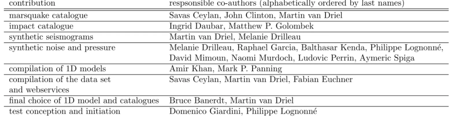
Table 1: Contributions to the blind test data set
contribution respsonsible co-authors (alphabetically ordered by last names)
marsquake catalogue Savas Ceylan, John Clinton, Martin van Driel
impact catalogue Ingrid Daubar, Matthew P. Golombek
synthetic seismograms Martin van Driel, Melanie Drilleau
synthetic noise and pressure Melanie Drilleau, Raphael Garcia, Balthasar Kenda, Philippe Lognonn´e,
David Mimoun, Naomi Murdoch, Ludovic Perrin, Aymeric Spiga
compilation of 1D models Amir Khan, Mark P. Panning
compilation of the data set Savas Ceylan, Martin van Driel, Fabian Euchner
and webservices
final choice of 1D model and catalogues Bruce Banerdt, Martin van Driel
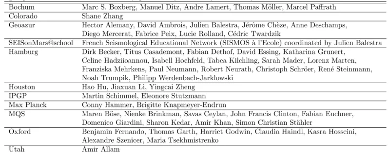
Table 2: Participating teams and their members
group name team members (alphabetically ordered by last names)
Bochum Marc S. Boxberg, Manuel Ditz, Andre Lamert, Thomas M¨oller, Marcel Paffrath
Colorado Shane Zhang
Geoazur Hector Alemany, David Ambrois, Julien Balestra, J´erˆome Ch`eze, Anne Deschamps,
Diego Mercerat, Fabrice Peix, Lucie Rolland, C´edric Twardzik
SEISonMars@school French Seismological Educational Network (SISMOS `a l’Ecole) coordinated by Julien Balestra
Hamburg Dirk Becker, Titus Casademont, Fabian Dethof, David Essing, Katharina Grunert,
Celine Hadziioannou, Isabell Hochfeld, Tabea Kilchling, Sarah Mader, Lorenz Marten,
Franziska Mehrkens, Paul Neumann, Robert Neurath, Christoph Schr¨oer, Ren´e Steinmann,
Noah Trumpik, Philipp Werdenbach-Jarklowski
Houston Hao Hu, Jiaxuan Li, Yingcai Zheng
IPGP Martin Schimmel, Eleonore Stutzmann
Max Planck Conny Hammer, Brigitte Knapmeyer-Endrun
MQS Maren B¨ose, Nienke Brinkman, Savas Ceylan, John Francis Clinton, Fabian Euchner,
Domenico Giardini, Sharon Kedar, Amir Khan, Simon Christian St¨ahler
Oxford Benjamin Fernando, Thomas Garth, Harriet Godwin, Claudia Haindl, Kasra Hosseini,
Alexandre Szenicer, Maria Tsekhmistrenko
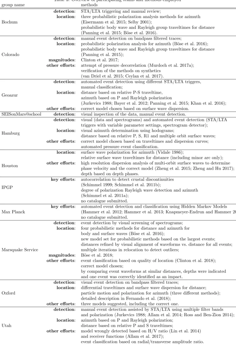
Table 3: Overview of participating teams and methods employed
group name methods
Bochum
detection: STA/LTA triggering and manual review;
location: three probabilistic polarization analysis methods for azimuth
(Eisermann et al. 2015; Selby 2001);
probabilistic body wave and Rayleigh group traveltimes for distance
(Panning et al. 2015; B¨ose et al. 2016).
Colorado
detection: manual event detection on bandpass filtered traces;
location: probabilistic polarization analysis for azimuth (B¨ose et al. 2016);
probabilistic body wave and Rayleigh group traveltimes for distance (Panning et al. 2015);
magnitudes: Clinton et al. 2017;
other efforts: attempt of pressure decorrelation (Murdoch et al. 2017a);
verification of the methods on synthetics (van Driel et al. 2015; Ceylan et al. 2017).
Geoazur
detection: automated event detection using different STA/LTA triggers,
manual classification;
location: distance based on relative P-S traveltime,
azimuth based on P and Rayleigh polarization
(Jurkevics 1988; Bayer et al. 2012; Panning et al. 2015; Khan et al. 2016);
other efforts: correct model chosen based on surface wave dispersion.
SEISonMars@school detection: visual inspection of the data, manual event detection.
Hamburg
detection: visual (data and spectrograms) and automated event detection (STA/LTA
triggers with variable parameter settings, spectrogram detector);
location: visual azimuth determination using hodograms;
distance based on relative P, S, R1 and multiple orbit surface waves;
other efforts: correct model chosen based on traveltimes and dispersion curves;
automated pressure event classification.
Houston
location: surface wave polarization for azimuth (Vidale 1986);
relative surface wave traveltimes for distance (including minor arc only);
other efforts: high resolution dispersion analysis of multi-orbit surface waves to determine
phase velocity and the correct model (Zheng et al. 2015; Zheng and Hu 2017); depth based on depth phases.
IPGP
key efforts: autocorrelation to detect crustal discontinuities
(Schimmel 1999; Schimmel et al. 2011b);
degree of polarization Rayleigh wave detection and azimuth (Schimmel et al. 2011a);
no catalogue submitted. Max Planck
key efforts: automated event detection and classification using Hidden Markov Models
(Hammer et al. 2012; Hammer et al. 2013; Knapmeyer-Endrun and Hammer 2015); no catalogue submitted.
Marsquake Service
detection: event detection by visual screening of spectrograms;
location: four probabilistic methods for distance and azimuth for
body and surface waves (B¨ose et al. 2016);
new model set for probabilistic methods based on the largest events;
distances refined by visual alignment of waveforms vs. distance for all events; multiple iterations in relocation to detect outliers;
magnitudes: B¨ose et al. 2018;
other efforts: event classification based on quality of location (Clinton et al. 2018);
correct model chosen;
by comparing event waveforms at similar distances, depths were indicated and one event was correctly identified as an impact.
Oxford
detection: visual event detection on bandpass filtered traces;
location: differential traveltimes and surface wave dispersion for distance;
particle motion and polarization for azimuth (three different methods); detailed description in Fernando et al. (2018);
other efforts: three models suggested, including the correct one.
Utah
detection: manual event detection assisted by STA/LTA using multiple filter bands
and polarization (Jurkevics 1988; Allam et al. 2014; Ross and Ben-Zion 2014);
location: azimuth based on P and Rayleigh polarization;
distance based on relative P and S traveltimes;
other efforts: model wrongly detected based on H/V ratio (Lin et al. 2014)
and receiver functions (Allam et al. 2017);
M3
M4
M5
8 16 24 32 40 48 56 64 72 Depth(km) -180° 180° -180° 180°Figure 1: Catalogue summary maps: distribution of impacts (left) and marsquakes (right) in the true catalogue, both randomly distributed over the sphere. The maps are centered on the InSight landing site (white triangle). Only a fraction of these events were detectable above the noise level.
2.0 2.5 3.0 3.5 4.0 4.5 5.0 5.5 Mw 1 0 1 2 3 4 5 log(Cum.N) b-value ( N=204) Reference b-value=1.0 Catalog b-value=1.03 N per magnitude bin
0 5 10 15 20 25 30 35 40 N per bin 2.5 3.5 4.5 Mw 0 20 40 60 80 100 Depth(km) Marsquake N per bin
0 10 20 N per depth bin30 40 50 60
Figure 2: Statistics for marsquakes in the true catalogue: (left) The magnitude-frequency distribution approximates a
Gutenberg-Richter distribution with b-value 1.0. The largest event in the catalogue has a magnitude Mw = 5.0. (right)
The magnitude-depth distribution of the marsquakes in the true catalogue is a skewed Gaussian with a maximum event number around 20 km and maximum allowed event depth of 80 km.
0 2 4 6 8 10 0 500 1000 1500 2000 2500 3000 Depth / km
Velocity / (km / s), Density / (10³ kg / m³) Traveltime / s A VP VS RHO 0 5 0 5 10 15 20 25 30 0 500 1000 1500 2000 2500 0 45 90 135 180 Distance / degr ee C SS S PP P 0 100 200 300 0 5 10 15 20 0 50 100 150 200 250 300 350 2.5 3.0 3.5 4.0 4.5 V elocity / ( km / s) B Rayleigh phase Rayleigh group Love phase Love group bedrock = 1km moho = 85 km
core mantle boundary= 1671.5 km orthopyroxene >
high pressure polymorph of clinopyroxene
olivine > wadsleyite
wadsleyite > ringwoodite Period / s
Figure 3: Summary of the model EH45TcoldCrust1b that was used in the blind test. Vertical profile of (A) seismic velocities and density, (B) dispersion curves, and (C) travel times. This model includes a low-velocity zone (LVZ, a region with a negative velocity gradient for either or both P and S). The LVZ leads to broad shadow zones for direct-arriving S-phases as indicated by gaps in the travel time curves in (C).
P PP S SS Rayleigh Love
Time (s) Time (s) Time (s)
P-coda / guided wave Rayleigh 1st overtone
Figure 4: The most visible events in the data set, plotted as a function of distance from the station. Travel time curves for the most prominent phases are shown in the legend. The waveforms are bandpass filtered between 1.5 and 10 s.
Bochum Colorado Geoazur
SEISonMars@school
Hamburg Houston Max Planck
MQS
Oxford
Utah
0
20
40
60
80
100
Number of Events
events in catalogue
correct detections
location provided
within L1
Figure 5: Summary of the team performances: total number of detected events in the submitted catalogues (blue); detected events that can be associated with an event in the true catalogue (orange); detected events in the submitted catalogues with full locations provided (green); and number of these events that lie within L1 mission requirements (red). Note the difference between orange and blue indicates false detections.
3 4 5
Bochum
all quakes correct location correct detection double detection false detection 3 4 5Colorado
3 4 5Geoazur
3 4 5SEISonMars@school
3 4 5Hamburg
3 Mw4 5Houston
3 4 5Max Planck
3 4 5MQS
3 4 5Oxford
0 50 100 150 200 250 300 350 Julian day 3 4 5Utah
6 7 8 all impacts correct location correct detection 6 7 8 6 7 8 6 7 8 6 7 8 6 7 8 log10 p 6 7 8 6 7 8 6 7 8 6 7 8 Figure 6: T emp oral o v erview of the submitted catalogues indicating correct detections and lo cations as w ell as double and false detections. All ev en ts in the true catalogue are sho wn, red and green corresp ond to correct detection and correct lo cation, those in gra y are missing in the submitted catalogue. Marsquak es are sho wn as circles, and impacts as stars. Note the scale based on linear momen tum p for the impacts on the righ t hand side.0 30 60 90 120 150 180 Distance( ) 2.5 3.0 3.5 4.0 4.5 5.0 Mw MQS outside L1 reqs. MQS within L1 reqs. True event Outside L1 reqs. Within L1 reqs. (a) Bochum 0 30 60 90 120 150 180 Distance( ) 2.5 3.0 3.5 4.0 4.5 5.0 Mw MQS outside L1 reqs. MQS within L1 reqs. True event Outside L1 reqs. Within L1 reqs. (b) Geoazur 0 30 60 90 120 150 180 Distance( ) 2.5 3.0 3.5 4.0 4.5 5.0 Mw MQS outside L1 reqs. MQS within L1 reqs. True event Outside L1 reqs. Within L1 reqs. (c) Hamburg 0 30 60 90 120 150 180 Distance( ) 2.5 3.0 3.5 4.0 4.5 5.0 Mw MQS outside L1 reqs. MQS within L1 reqs. True event Outside L1 reqs. Within L1 reqs. (d) Houston 0 30 60 90 120 150 180 Distance( ) 2.5 3.0 3.5 4.0 4.5 5.0 Mw MQS outside L1 reqs. MQS within L1 reqs. True event Outside L1 reqs. Within L1 reqs. (e) MQS 0 30 60 90 120 150 180 Distance( ) 2.5 3.0 3.5 4.0 4.5 5.0 Mw MQS outside L1 reqs. MQS within L1 reqs. True event Outside L1 reqs. Within L1 reqs. (f) Oxford
Figure 7: Distance-magnitude summary for the six most complete submitted catalogues. All events in the true catalogue are shown for each team, correctly detected in red, correctly located in green and missed events in gray. The dashed lines approximate the detection threshold (gray dashed line) and correct location threshold (black dashed line) for MQS. Histograms at the top and right side show the number of correctly detected (red), correctly located (green) and missed events (gray) for a number of distance and magnitude bins.
0 30 60 90 120 150 180 True distance( ) 0 20 40 60 80 100 120 140 160 180 Co m pu te d dis ta nc e( ) Within L1 reqs. Outside L1 reqs. InSight L1 reqs. (a) Bochum 0 30 60 90 120 150 180 True distance( ) 0 20 40 60 80 100 120 140 160 180 Co m pu te d dis ta nc e( ) Within L1 reqs. Outside L1 reqs. InSight L1 reqs. (b) Geoazur 0 30 60 90 120 150 180 True distance( ) 0 20 40 60 80 100 120 140 160 180 Co m pu te d dis ta nc e( ) Within L1 reqs. Outside L1 reqs. InSight L1 reqs. (c) Hamburg 0 30 60 90 120 150 180 True distance( ) 0 20 40 60 80 100 120 140 160 180 Co m pu te d dis ta nc e( ) Within L1 reqs. Outside L1 reqs. InSight L1 reqs. (d) Houston 0 30 60 90 120 150 180 True distance( ) 0 20 40 60 80 100 120 140 160 180 Co m pu te d dis ta nc e( ) Quality A Quality B Quality C
Quality B Outside L1 reqs. Quality C Outside L1 reqs. InSight L1 reqs. (e) MQS 0 30 60 90 120 150 180 True distance( ) 0 20 40 60 80 100 120 140 160 180 Co m pu te d dis ta nc e( ) Within L1 reqs. Outside L1 reqs. InSight L1 reqs. (f) Oxford
Figure 8: Distance performance - comparing the distances provided in the six most complete submitted catalogues with the true event distance. Gray area marks the L1 requirement. Note that for an event to be located within L1 we also required correct azimuth and origin time. For MQS, their data quality classification is indicated.
0 30 60 90 120 150 180 Distance ( ) 180 90 200 20 90 180 BA Z er ro r( ) Within L1 reqs. Outside L1 reqs. InSight L1 reqs. (a) Bochum 0 30 60 90 120 150 180 Distance ( ) 180 90 200 20 90 180 BA Z er ro r( ) Within L1 reqs. Outside L1 reqs. InSight L1 reqs. (b) Geoazur 0 30 60 90 120 150 180 Distance ( ) 180 90 200 20 90 180 BA Z er ro r( ) Within L1 reqs. Outside L1 reqs. InSight L1 reqs. (c) Hamburg 0 30 60 90 120 150 180 Distance ( ) 180 90 200 20 90 180 BA Z er ro r( ) Within L1 reqs. Outside L1 reqs. InSight L1 reqs. (d) Houston 0 30 60 90 120 150 180 Distance ( ) 180 90 200 20 90 180 BA Z er ro r( ) Quality A Quality B Quality C
Quality B Outside L1 reqs. Quality C Outside L1 reqs. InSight L1 reqs. (e) MQS 0 30 60 90 120 150 180 Distance ( ) 180 90 200 20 90 180 BA Z er ro r( ) Within L1 reqs. Outside L1 reqs. InSight L1 reqs. (f) Oxford
Figure 9: Back-azimuth performance for the six most complete submitted catalogues in terms of the back-aimuth estimation error as a function of distance. The gray area marks the mission L1 requirement. Note that for an event to be located within L1 we also required correct distance and origin time.
0 30 60 90 120 150 180 Distance ( ) 1500 1250 1000 750 500 250 0 250 500 750
Origin time error (s)
Within L1 reqs. Outside L1 reqs. (a) Bochum 0 30 60 90 120 150 180 Distance ( ) 1500 1250 1000 750 500 250 0 250 500 750
Origin time error (s)
Within L1 reqs. Outside L1 reqs. (b) Geoazur 0 30 60 90 120 150 180 Distance ( ) 1500 1250 1000 750 500 250 0 250 500 750
Origin time error (s)
Within L1 reqs. Outside L1 reqs. (c) Hamburg 0 30 60 90 120 150 180 Distance ( ) 1500 1250 1000 750 500 250 0 250 500 750
Origin time error (s)
Within L1 reqs. Outside L1 reqs. (d) Houston 0 30 60 90 120 150 180 Distance ( ) 1500 1250 1000 750 500 250 0 250 500 750
Origin time error (s) Quality AQuality B Quality C
Quality B Outside L1 reqs. Quality C Outside L1 reqs.
(e) MQS
Figure 10: Origin time performance for the five most complete submitted catalogues in terms of the timing error as a function of distance. Note that there is no L1 requirement, but for an event to be located within L1 we required correct azimuth and distance. Oxford’s catalogue did not include origin times, but only arrival times; hence it is omitted here.
0 200 400 600 800 1000 2 1 0 1 2 31e 9 Computed ∆=13.0° True ∆=7.1° Bandpass at 1.5-10.0 s.
Z-component
P1 S1(on T comp.) Computed OT True OT 200 0 200 400 600 800 1000 1200 1400 1.0 0.5 0.0 0.5 1e 8 True ∆=12.7° Bandpass at 1.5-10.0 s. 0 1000 2000 3000Time after origin(s) 2.0 1.5 1.0 0.5 0.0 0.5 1.0 1.5 2.0 Velocity(m/s) 1e 9 True ∆=20.6° Bandpass at 1.5-10.0 s. 0 50 100 150 200 250 300 6 4 2 0 2 4 61e 9 Computed ∆=2.9° True ∆=3.2° Mw=2.5, Depth=74.1 km Bandpass at 1.5-10.0 s.
Z-component
G1(on T comp.) P1 R1 S1(on T comp.) Computed OT True OT 0 500 1000 1500 2000 4 2 0 2 4 1e 6 Computed ∆=35.4° True ∆=35.1° Mw=5.0, Depth=16.8 km Bandpass at 1.5-30.0 s. 0 1000 2000 3000 4000Time after origin(s) 3 2 1 0 1 2 3 4 Velocity(m/s) 1e 9 Computed ∆=109.9° True ∆=109.6° Mw=3.6, Depth=21.0 km Bandpass at 1.5-10.0 s.
Figure 11: (top) Location and vertical component waveforms for the three strongest impact signals in the true catalogue. On the map, the impacts are indicated by stars (size proportional to the linear momentum), the station is marked with the triangle. The closest event was correctly identified as an impact by MQS. Though some other teams identified the largest event, no other team classified it as an impact in their catalogues. (bottom) Similar plot for three quakes for comparison. Seismic phases in both plots are annotated as: S1/P1 - first arriving S/P wave, where S was only visible on the tranverse component, G1/R1 - minor arc Love/Rayleigh waves, OT - source origin time.