OATAO is an open access repository that collects the work of Toulouse
researchers and makes it freely available over the web where possible
Any correspondence concerning this service should be sent
to the repository administrator: [email protected]
This is an author’s version published in: http://oatao.univ-toulouse.fr/21989
To cite this version:
Soualhi, Abdenour
and Hawwari, Yasmine and Medjaher,
Kamal
and Clerc, Guy
and Hubert, Razik
and Guillet,
François
PHM survey: implementation of signal processing
methods for monitoring bearings and gearboxes. (2018)
International Journal of Prognostics and Health Management, 9 (2).
ISSN 2153-2648
PHM Survey : Implementation of Signal Processing Methods for
Monitoring Bearings and Gearboxes
Abdenour Soualhi1, Yasmine Hawwari2, Kamal Medjaher3, Guy Clerc4, Razik Hubert4 and François Guillet1 1Univ Lyon, UJM-Saint Etienne, Saint-Etienne, France
[email protected] [email protected]
²Univ d'Orlèans, Laboratoire PRISME, Orlèans, France
3ENIT - LGP, Tarbes, France [email protected] 4
Univ Lyon, Univ Lyon-1, Laboratoire Ampère, France
ABSTRACT
The reliability and safety of industrial equipments are one of the main objectives of companies to remain competitive in sectors that are more and more exigent in terms of cost and security. Thus, an unexpected shutdown can lead to physical injury as well as economic consequences. This paper aims to show the emergence of the Prognostics and Health Management (PHM) concept in the industry and to describe how it comes to complement the different mainten-ance strategies. It describes the benefits to be expected by the implementation of signal processing, diagnostic and prognostic methods in health-monitoring. More specifically, this paper provides a state of the art of existing signal processing techniques that can be used in the PHM strategy. This paper allows showing the diversity of possible tech-niques and choosing among them the one that will define a framework for industrials to monitor sensitive components like bearings and gearboxes.
1. INTRODUCTION
ance (CBM), is defined as an approach for the health man-agement of systems based primarily on the diagnostic, prognostic and decision-making in maintenance. This phi-losophy is relatively new since the PHM community emerged in the early 2000s to form the PHM Society and IEEE PHM. Following the researches of Niu et al. (2010), Jaloretto et al. (2009), Appleby (2003), Yu et al. (2007) and Kumar et al. (2010), the objectives behind the implementa-tion of a PHM philosophy are:
- A better availability and, thus, a reduction in costs operat-ing and maintenance through a policy of maintenance and logistics based on the monitoring of the health status of equipment or system in real time;
- A faster detection of degradation or loss of performance for an efficient operating;
- An improvement of the reliability and the security of criti-cal components;
- A reduction of logistics congestion and costs associated with the maintenance materials, transportation, stock, and maintenance personnel;
- A failure reduction induced by maintenance;
- A forecasting and quantification of the future degradation to provide a way to quantify the remaining life of systems. This helps to identify those which are near their end of life and require significant capital expenditures to differentiate them from those that do not require a simple restoration.
PHM allows maintenance to be performed more effi-ciently by integrating PHM data (eg. the RUL "Remaining Useful Life") from the prognostic and the location and iden-tification of failures resulting from the diagnostic and health assessment derived from detection, maintenance data (re-sources and inventories), logistical constraints and informa-Prognostics and Health Management (PHM) is an
emerg-ing "philosophy" which extends the concept of predictive maintenance by optimizing the maintenance and the logistic support to increase the reliability and life expectancy of mechanical, structural and electronic systems while Life-Cycle costs are reduced and operational availability is in-creased (Kalgren et al., 2006, Kim et al., 2017). This philos-ophy, usually confused with the Condition Based
Mainten-Abdenour SOUALHI et al. This is an open-access article distributed under the terms of the Creative Commons Attribution 3.0 United States License, which permits unrestricted use, distribution, and reproduction in any me-dium, provided the original author and source are credited.
tion on the planned mission. The historical failure provides a database of failure models. These models are used for assessing current equipment information to determine the likely cause for any anomalies detected in the equipment. The RUL database is used to construct life prediction mod-els. These models are used to analyze current equipment information to estimate its remaining useful service life. This is the typical architecture of a PHM system. It is usual-ly formalized with the standard OSA-CBM (Open System Architecture for Condition Based Maintenance) (see Bengtsson, 2003, Thurston, 2001a, Rasovska et al., 2007 and Swearingen et al., 2007). This architecture establishes a framework communication between the monitoring system and the various experts concerned through industrial main-tenance (Holmberg et al., 2010).
In fact, it is suitable to expose the evolution of mainten-ance types (Elghazel et al., 2015). The earlier shape of maintenance is corrective maintenance which consists of reacting only when the equipment fails. Thus, this strategy will lead to sudden breakdowns. So, the time-based or pre-ventive maintenance was invented. The Prepre-ventive Main-tenance is defined as a "MainMain-tenance carried out at prede-termined intervals or according to prescribed criteria and intended to reduce the rate of failure or degradation of equipment" (SS-EN 13306, 2001, p.14). Preventive main-tenance includes two types of mainmain-tenance plans: systematic preventive maintenance and condition based maintenance (SS-EN 13306, 2001). Systematic maintenance is scheduled and planned without the occurrence of any monitoring activ-ity. It could be based on the number of hours of use, the number of times that a system is used, the number of kilo-meters of use, depending on prescribed dates and so on. This type of service is best suited for a component that has visible signs of wear and where maintenance tasks can be performed at a time that will prevent a system failure (Starr, 1997). According to Yam et al. (2001) and Starr (1997), systematic maintenance is sometimes called "time-based maintenance" and "planned preventive maintenance". Since time-based maintenance doesn’t take into account the state of the system, it was necessary to come up with condition based maintenance discussed in nineties (Heng et al., 2009). Condition based maintenance (CBM), in contrast to the systematic maintenance, is not based on planned actions. It is carried out according to the needs identified by the system health (Yam et al., 2001). It is based on parameters (fea-tures) that can detect the current health and used to predict possible failures before their real occurrence. The monitor-ing of these features can provide an indication of an im-pending failure as well as emerging defects that can lead the system or its components to deviate from an acceptable level of performance or in the worst case, cause its degrada-tion. Among the advantages of the CBM, making the right maintenance actions which avoids stopping a healthy system functioning (Heng et al., 2009), its ability to detect an im-minent fault and accuracy predicting failures (Soualhi et al., 2014). It also contributes to fault diagnosis because it is relatively easy to associate a specific defect in the system to the monitored features.
So, the PHM associated with the CBM can significantly reduce the costs of intervention and increase the dependabil-ity of systems. These results are achieved only if all layers composing the CBM are operational. One of the most im-portant layer is the signal processing. This implies a good knowledge of the different signal processing techniques used to extract fault indicators. Hence, this paper details the signal processing layer of the CBM architecture and pro-vides an extensive state of the art of existing techniques used in the PHM strategy. Thus, it lists the various possible techniques and establishes the choice that will represent a solid framework for industrial applications using sensitive components like bearings and gearboxes. Therefore, sec-tions of this work revolve around the detailed presentation of the different signal processing techniques and their cate-gorization. The next section present in detail the different layers composing the CBM. The section 3 will be dedicated to the presentation of the different signal processing tech-niques.
2. IMPLEMENTATION OF A CONDITIONAL BASED MAIN-TENANCE (CBM)
A conditional based maintenance is composed of seven layers: data acquisition, signal processing, health assess-ment, diagnostic, prognostic and decision support. The se-venth layer is called the human-machine interface (HMI). It is not essential for the CBM but allows displaying vital information about the health status of the system. The (MI-MOSA) "Machinery Information Management Open Stan-dard Alliance" has been proposed as a stanStan-dardized architec-ture for the CBM described in six functional layers: from the data acquisition to the decision support module (Thurs-ton., 2001b).
+ Layer 1 - The data acquisition module provides access to signals (digital data) from sensors. The data acquisition covers different disciplines such as mechanical measure-ments (Wang & McFadden, 1996, Holroyd, 2005, Roemer & Kacprzynski, 2000, Hountalas, 2000), electrical mea-surements (Tsoumas et al., 2005, Kar & Mohanty, 2006), tribology (Walter & Lee, 2004) and non-destructive mea-surements (Mba, 2006). The mechanical meamea-surements include mechanical vibration, acoustic emission, pressure, flow, temperature, and stress, while the electrical measure-ments are current, voltage, phase and flux. Tribology is especially interested in the machinery lubrication and oil analysis of debris. The non-destructive control uses visual inspection or non-contact measurement.
+ Layer 2 – The signal processing module receives signals from the data acquisition module. The outputs of this mod-ule are health indicators extracted from signal processing techniques: temporal analysis, spectral analysis, time-frequency analysis.
+ Layer 3 - The health assessment module receives data from the signal processing module and other monitoring modules. The aim is to compare the extracted health indica-tors with reference values to assess the condition of the machine. The health assessment module generates alarms
based on predefined operating limits (eg, low level of de-gradation, natural degradation level and advanced stage of degradation).
+ Layer 4 - The diagnostic module receives data from the signal processing and health assessment modules. Based on the obtained indicators, this module determines whether the state of the monitored system or component is degraded or not and identify the element responsible of this degradation. + Layer 5 - The prognostic module considers information provided from all previous layers to estimate the remaining useful life (RUL) of the system. The RUL is obtained by extrapolating a series of measurements (time series) from a health indicator acquired until a present time "t" to a horizon of prediction defined by t+RUL. t+RUL corresponds to the moment where the extrapolated time series reached the threshold of system’s degradation.
+ Layer 6 - The decision support module receives data from the diagnostic and prognostic modules. This module gives recommend maintenance actions and alternatives related to the management of the system.
In the next section, the main focus will be on the second layer, which is the signal processing .
3. SIGNAL PROCESSING
As said in the introduction section, the signal processing is one of the most important module of the CBM. This module analyzes and transforms the input signal to extract indicators of defects (Seryasat et al., 2010, Chen et al., 2012, Prieto et al., 2013). From the literature, several processing techniques, like temporal analysis, frequency analysis and time-frequency analysis can be used to extract efficient health indicators (Tobon-Mejia et al., 2012, Niu & Yang, 2010, Tsui et al., 2015).
3.1.Temporal analysis
The temporal analysis extracts indicators of defect from raw signals. These features are called "statistical indicators" because they represent the temporal characteristics of the recorded signal. Table 1 shows a list of the most common indicators used in the time-domain:
Peak value 1,..., ˆ sup | i| i N x x = = Crest indicator 1 ˆ (1 ) iN( )²i x CI N = x =
∑
Mean 1 1 N i i x x N = =∑
Standard deviation 1 1 ( )² 1 N i i x x N σ = = − −∑
Shape indicator 1 1 (1 ) ( )² (1 ) | | N i i N i i N x SI N x = = =∑
∑
Root mean square 1 1 ( )² N i i RMS x N = =∑
Impulse Indicator 1 ˆ (1 ) iN| i| x IM N = x =∑
Skewness 3 1 3 ( ) ( 1) N i i x x SK N σ = − = −∑
Kurtosis 4 1 4 ( ) ( 1) N i i x x KU N σ = − = −∑
Table 1. Statistical features (Chen et al., 2012).where xi is the i-th sample of the recorded signal x(t) and N
is the number of samples.
The most popular indicators used in literature are: - The standard deviation σ which measure the dispersion of the signal x(t). This indicator is often used as a metric in classifiers such as dynamic Bayesian networks (Wang et al., 2007) and neural networks (Laerhoven et al., 2001).
- The RMS is the most interesting measure of vibration amplitudes. In addition of taking into account the evolution of the signal over time, the calculation of the RMS value is related to the vibratory energy and therefore to the "poten-tial for deterioration" of the vibration signal. In practice, the positive and negative instantaneous values of the signal are squared. The average of these values is then calculated over a certain period of time. The result is put under the square root to obtain the RMS. Recently, the RMS was used to verify the effectiveness of exploiting only a selection of the vibration signals instead of the original ones. Results showed that when RMS is applied after the selection step, it gives more significant information about the faulty cases (Feng et al., 2017).
In Hemmati et al. (2016), authors investigate the effec-tiveness of this parameter to detect bearing faults compared to other statistical parameters like peak value, kurtosis, crest factor and skewness. Bearing faults are artificially produced on an outer race using an engraving machine tool to control the shape and depth of the faults. In this experimentation, defect size, rotating speed, and radial load have been consi-dered as the most critical parameters that may influence the statistical parameters. Results showed that since in many practical cases the rotating speed of the shaft is constant, RMS is a strong candidate for identifying defective rolling element bearings.
- The Skewness, commonly called the moment of order 3, is mathematically defined by the the ratio of the average cubed deviation from the mean divided by the cube of the standard deviation. This definition represents the dissymmetry rate of the amplitude distribution of the signal with respect to a maximum (whose abscissa corresponds to the mean in the case of a Gaussian). The measurement of this dissymmetry is given in table 1. It is a dimensionless quantity. The Skewness will be positive or negative depending on the distribution of the curve to the right or left, respectively, of the mean value. If the Skewness is equal to 0, the distribu-tion is symmetric. If the Skewness is smaller than 0, the distribution is shifted to the left compared to its mean. If the Skewness is greater than 0, the distribution is shifted to the right. It was proven in the paper of Hemmati et al. (2016) that the Skewness is a good indicator for diagnosing bearing faults.
- The kurtosis represents the relation between the statistical moment of order 4 and the square of the statistical moment of order 2. For a Gaussian distribution, the Kurtosis is equal to 3 (case of a healthy bearing or gear). When the signal becomes non-Gaussian (appearance of a fault) the kurtosis becomes greater than 3 (see table 2). The Kurtosis is an indicator of impulsivity, it is independent of the amplitudes
and it allows possible establishing a criterion of severity for the diagnosis of machines (Thomas, 2002). For the sake of comparison, Pang et al. (2018) used the Kurtosis for the same fault case but before and after the improved version of the proposed framework and found out that it gives signifi-cant values in the second case.
Kurtosis Severity
1,5 Good
2,8 to 3,2 Acceptable 3,2 to 4 High
> 4 critical
Table 2. quantification of the severity according to kurtosis. - The crest indicator is the ratio between the peak amplitude of the signal and the RMS. A system in a good condition generates a low amplitude signal as well as in the peak value and the RMS. The crest factor remains low (between 2 and 6). A localized defect generates a high peak amplitude and low RMS amplitude, so an important peak factor (greater than 6). However, as the RMS increases for progressive failure, the crest indicator decreases (Dron et al., 2004).
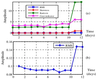
The Kurtosis, Skewness, CI and RMS have been ex-tracted from vibration signals to detect the degradation of the gearbox. The degradation test was done for a duration of 12 days. These indicators are given in fig.1:
Figure 1. a) Curves of the kurtosis, skewness, CI and RMS of a faulty gearbox. b) A zoom on RMS curve. These curves show the beginning of the degradation after the 8th day followed by an increase until the apparition of the degradation in the 12th day.
Another indicator called the Entropy can be added to ta-ble 1. The different types of the entropy have been devel-oped in Han et al. (2009) for the indicator extraction. Table 3 shows the most used entropy types:
Shannon entropy ² log( ²)
i i
i
x x
−
∑
Log energy entropy log( ²)
i i
x
∑
Table 3. Entropy features.To improve the effectiveness of these indicators, a tem-poral analysis tool called the time synchronous average (TSA) was introduced by Bennett (1958). The TSA was applied for cyclostationary vibration signals for fault detec-tion of gearbox. The TSA consists of dividing a vibradetec-tion signal into time-segments and carrying out a mean of these segments to eliminate the noise. In Bonnardot (2004), the angular synchronous average (ASA) was proposed. The ASA consists of dividing a vibration signal into angular-segments. This approach was tested in a gearbox and the obtained results are better than the TSA.
Another method has been proposed in Hong and Dhupia (2014). It consists of combining the fast-dynamic time warping (Fast DTW) and the correlated kurtosis (CK) tech-niques to detect and identify the faulty gear. Considering that the faulty gear tooth generates periodic impulses in the vibration signal, the fast DTW extracts these impulses by using a reference signal at the same frequency of the nomin-al gear mesh harmonic. It is based on vibration signnomin-als ob-tained from a healthy and steady functioning of the system. Then, the subsequent signal is resampled for the diagnostic by the CK technique which aims to isolate the gearbox fault locally by analyzing the periodic effect of the fault.
Another method was developed in Do and Chong (2011). It consists of transforming a vibration signal (one-dimensional domain) into an image (two-(one-dimensional) by translation. The indicators are deduced by the scale invariant feature transform (SIFT) to detect faults by affecting the vibration signal to the corresponding fault category (diagno-sis level). For the translation (see fig. 2), the amplitude samples of the signal are normalized to obtain values in the range [0-255]. These values are putted in a matrix M*N where the coordinate of the ith element in the vibration signal is the pixel (j,k) in the matrix with j = floor (i/N) and k = modulo (i/N). Then the SIFT algorithm is applied on this image to obtain 128-dimension vectors. Finally, each indica-tor vecindica-tor is compared to each centroid of the fault category dictionary to obtain a histogram of similarity between the indicator vectors and the fault category. The fault category of the vibration signal corresponds to the highest similarity. Figure 3 gives an example of this method.
Figure 2. Vibration signal to image translation scheme (Averbuch & Zheludev, 2002).
2 4 6 8 10 12 0 5 10 RMS Skewness Kurtosis Crest indicator 0 2 4 6 8 10 12 0.08 0.1 0.12 0.14 0.16 RMS Time (da ys) Time (da ys) A m p lit u d e A m p lit u d e (a ) (b) m a g n it u d e
Signal in time domain Image (size(M×N) Pixel [0,0] 0 1 2 3 N-1 0 1 2 3 M-1 0 1 2 3 N N+1
Figure 3. An example of vibration signal translated into the 128-128 gray image (M=128 and N=128) (Averbuch and
Zheludev, 2002).
An important concept widely used in bearing and gear diagnostic is the cyclostationarity. It was applied to helicop-ter gearbox in Antoni and Randall (2002) in order to sepa-rate the periodic components of the signal from the random ones. This leads to the definition of first-order cyclostatio-narity (CS1) related to deterministic signals such as gear signals and second-order cyclostationarity (CS2) related to random signals such as bearing signals. Very recently, Ca-soli et al. (2018) applied the angular synchronous average on the acceleration signals and decomposed it into CS1 and CS2 for fault detection of hydraulic axial piston pumps and studied the impact of faults on both indicators. This hypo-thesis will generate new indicators that will be incorporated into diagnostic tools and prognosis to improve the PHM.
The extraction of features plays a major role in the effec-tiveness of the monitoring method. Therefore, researchers decided to mix different types of features. This is the case of Bleakie et al. (2013), where statistical features and dynamic features such as rise-time, overshoot and steady state values were chosen for system degradation prediction. The defini-tion of some dynamic features related to the time response of the system was given in detail by Franklin et al. (2010) .
The main advantage of the extracted indicators from temporal analysis is their capability to detect the degrada-tion of the system. However, the main drawback is their incapacity to identify the origin of the degradation. The frequency analysis tackles this point more efficiently than temporal analysis.
3.2.Frequency analysis
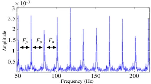
The spectrum analysis of a signal is the most common technique used to identify faults in electro-mechanical sys-tems. This technique is based on the fact that a localized defect generates a periodic signal with a unique characteris-tic frequency (Tandon & Choudhury, 1999). In contrast to the temporal analysis, the frequency analysis identifies this fault by locating the characteristic frequency of the fault. This technique is generally used during the steady state of the system (Didier, 2004). A classic tool among these tech-niques is the fast Fourier transform (FFT). Figure 4 shows an example of a faulty gearbox where the defect is located on the pinion with a series of pics separated with the pinion frequency Fp.
Figure 4. Spectrum of the acceleration signal of a faulty gearbox.
Another tool was proposed in Feng and Liang (2014) which is the demodulated spectra of the amplitude envelope. This tool detects and localizes faults by applying the FFT on the envelope of the signal. However, the Fourier transform is limited by the resolution (the frequency differences are much smaller than the inverse of the number of observed points). To resolve this problem, the algorithm MUSIC (Multiple signal characterization) was proposed in Schmidt (1986). MUSIC estimates the frequency content of a signal using an eigen space method. This method assumes that a signal, x(t), consists of p complex exponentials in the pres-ence of Gaussian white noise. Recently, Ma et al. (2018) used the Teager energy spectrum which is obtained by the application of the FFT on the Teager energy operator of the vibration signal and aims at envelope demodulation to achieve fault diagnosis of bearing. This operator calculates the energy of the signal at each time by using the data of three samples.
In an analogous way with the spectrum, another tool aims to detect system defects by the cepstrum (Oppenheim & Schafer, 2004). It is defined as the inverse Fourier transform (IFT) of the spectrum logarithm:
(
)
(
)
cepstrum of signal= IFT log FT the signal (1) Cepstrum analysis is used for fault extraction as it capa-ble to notice the periodic families in the frequency spectrum and represent it by specific peaks in the cepstrum. The first peaks are good indicators as they reflects a large amount of harmonics (Niu, 2017). This was previously exploited by proposing an indicator noted d(t) and called the normalized differential cepstral indicator (NDCI) was introduced by El Badaoui (1999). This NDCI uses the relative difference between the two cepstral pics in order to insure invariance regarding the additional noise. Figure 5 shows experimental results extracted from a gear box operating 12 days. As the sum of the energy of the two pics is constant, the amplitude corresponding to the gear defect increases while the other one decreases. From the NDCI curve, and giving that the NDCI tends to 1 when the pinion is faulty and to -1 when the gear wheel is faulty, this shows the appearance of a pinion fault at the 8th day. This fault continues to increase until the total spalling on all teeth.
0 0.2 0.4 0.6 0.8 1 -0.8 -0.6 -0.4 -0.2 0 0.2 0.4 0.6 m a g n it ud e time (sec) 128 1 2 8 150 100 200 50 Fp Fp Fp 3 2.5 2 1.5 1 0.5 × 10⁻³ 50 Frequency (Hz) A m pl it ud e 100 150 200
a) b) c)
Figure 5. A zoom on the first 2 pics in the cepstrum of a) day 1 b) day 8 c) day 12 temporal signals.
Recently, a technique called cepstrum editing procedure (CEP) was automated in Peeters et al. (2018). This method aims at separating deterministic signals from random ones, which can be very useful for bearings monitoring, as their components can be isolated from those of gears or shafts characterized by explicit peaks. In this paper, results were compared before and after the application of the automated CEP (ACEP) as a pre-processing step for envelope analysis and showed that adding ACEP helps for better interpretation of the bearing health.
The proposed signal processing techniques are generally applied on vibration signals but recently research was inter-ested to the use of electrical signals for fault detection and diagnosis (Bellini et al, 2008, Gong & Qiao, 2013, Saidi et al., 2012). A novel framework was developed in Leite et al. (2015). It consists of bearing fault detection of a three-phase induction motor by the squared envelope spectrum (SES) applied on the stator current. In order to enhance the envelope analysis, spectral kurtosis-based algorithms, were applied. Those algorithms are used in this method to resolve the problem of determining the filtering frequency band around the mechanical resonance of the machine (Barszcz & Jablonski, 2011, Sawalhi, 2007). The SES is obtained by applying the discrete Fourier Transform to the analytic sig-nal got from the Hilbert transform. Figure 6 illustrates the detection of a bearing outer race fault in an induction motor by the stator current SES where the outer race frequency and its harmonics are pointed by arrows.
Figure 6. SES of the stator current from the motor with a damaged bearing fault.
The main advantage of the frequency analysis is its capa-bility to locate the degraded component of the system. However, the main drawback is their incapacity to identify the origin of the degradation when the system is not statio-nary. This implies the use of the time-frequency analysis.
3.3.Time-frequency analysis
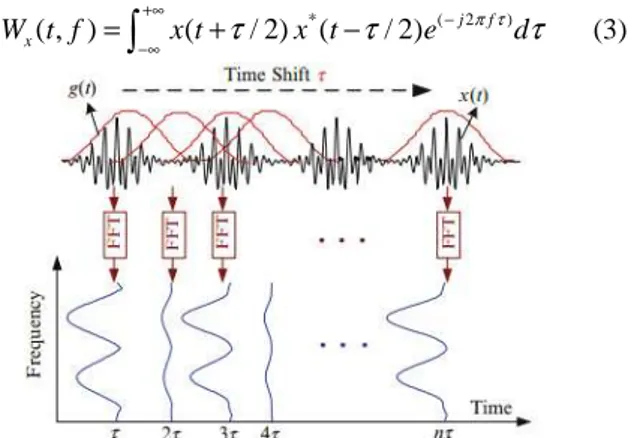
The time-frequency analysis covers both the time domain and the frequency domain. Non-stationary signals are better described by a time-frequency distribution to show the dis-tribution of the signal energy over the two-dimensional space-time-frequency (Burgess & Shimbel, 1995). The most commonly used techniques for time-frequency analysis is the short-time Fourier transform (STFT), the Wigner Ville distribution (WVD), wavelet transform (WT) and Hilbert– Huang transform (HHT). For example, the STFT method allows following the changing in frequency content in func-tion of time. This means that the defect becomes localizable in time. Although, this method needs high computational capacity when the quality of resolution matters. Since STFT is based on windowing the signal around a particular time t and calculating the Fourier transform for each time (see fig.7), this leads to make judicious choice of the window size with:
( 2 )
STFT( , ) ( ) ( ) j ft
f x t g t e π dt
τ =
∫
−τ − (2)where STFT can be interpreted as a similarity measure be-tween the signal x(t) and the time-delayed and frequency-modulated window g(t-τ).
The time-frequency analysis makes a compromise be-tween the time resolution and the frequency resolution. For the Wigner-Ville distribution, this compromise does not exist due to the absence of the window as we can see in the following equation: * ( 2 ) ( , ) ( / 2) ( / 2) j f x W t f +∞x t τ x t τ e− π τdτ −∞ =
∫
+ − (3)Figure 7. Illustration of short-time Fourier transform applied to signal x(t).
The main drawback of this method is that it is bilinear in nature, introducing the cross terms in the WVD domain, which make the transform difficult to interpret. The WVD of the sum of n signals
1 ( ) ( ) n i i x t x t = =
∑
is given by: 1 1 1 1 ( , ) ( , ) 2 Re ( , ) i k l n n n x x x x i k l kautocomponents cross component
W t f W t f W t f − = = = + − =
∑
+∑ ∑
14243 14444244443 (4)Cross terms could be reduced by processing the signal with a sliding window of time h(τ) in (3). This will suppress 0.059 0.168 0.0620.15 0.059 0.34 0.062 0.035 0.059 0.162 0.062 0.119 Frequency (Hz) A m p li tu d e
Outer race frequency
2 × Outer race frequency
3 × Outer race frequency
0 0 50 100 150 200 250 300 350 400 1 2 3 × 10⁻³ NDCI Time
the WVD components that oscillate in the frequency direc-tion. This method is called the pseudo Wigner-Ville distri-bution (PWVD). A further time-direction smoothing can be implemented by using an additional window in the frequen-cy domain h(f). This extend is called the Smoothed Pseuso Wigner Ville distribution (SPWVD) which realizes the best trade-off between resolutions (time and frequency) and the interferences. The SPWVD is considered as the compromise between STFT and WVD (Lee, 2013).
Another time-frequency technique is the Hilbert-Huang transform (HHT). The HHT is a combination of the empiri-cal mode decomposition (EMD) and the Hilbert spectral analysis (HSA). This technique performs an adaptive time-frequency technique and in the same time removes the noised signals to give useful information about the fault (Wang et al., 2014). The EMD uses the local characteristic time scales of a signal to extract the intrinsic mode functions (IMFs) (Lei et al., 2013). The IMFs are oscillatory functions with varying amplitude and frequency. They have the same length as the original signal and each IMF corresponds to a determined frequency range. Moreover, when the degrada-tion is at an early stage, the EMD are buried by the noise which constitutes the difficulty of earlier fault detection (Ali et al., 2015). The Hilbert spectral analysis is applied to the IMF to obtain the analytic form of the signal and after that, this signal is combined with the instantaneous frequency to obtain the Hilbert spectral density (HSD). In (Soualhi et al., 2015), authors used the Hilbert marginal spectrum in the IMF to extract bearing fault indicators by choosing the IMF which corresponds to the bearing characteristic frequencies. Furthermore, Zhu and Shen (2012) compared the Time-frequency techniques for non-stationary signals. The results of this comparison showed that the HHT is the most adap-tive to non-stationary signals. The HHT expresses a local information and instantaneous frequency in a high time-frequency resolution. Another comparison has been made by Li et al. (2016a). This paper compared different time-frequency techniques including STFT, WT, PWVD and HHT based on the quality representation but also on the execution time of each technique. The PWVD was the slowest.
In an analogous way with the EMD, local mean decom-position (LMD) was proposed as a self-adaptive time-frequency analysis method. LMD consists of decomposing a signal into a set of product functions (PFs) where each PF is the product of a frequency modulated frequency and its corresponding envelope component. Each PF is a mono-component amplitude modulated - frequency modulated (AM-FM) signal. In Park et al. (2011), complex local mean decomposition (CLMD) was developed to process not only real-valued signals but also complex valued signals. Expe-rimental results showed that LMD is capable of revealing information about amplitude and frequency with more accu-racy than EMD. This technique was also used in a method for fault diagnosis in Li et al. (2016b). This method consists of applying LMD on the signal to obtain product functions PFs and select the optimum PF which maximizes the
kurto-sis criterion. Then, the features of the chosen PF are calcu-lated by the improved multiscale fuzzy entropy (IMFE). The fuzzy entropy is defined to assess the complexity and irregu-larity of the time series. When it is applied on different scale factors, it is called IMFE (Li et al., 2017). The more signifi-cant features are selected by using Laplacien score (LS) algorithm which chooses automatically the best factor scale to reduce the dimensionality of features vectors. These new feature vectors are the input of the improved support vector machines to classify data into fault classes. This criterion may change from a framework to another; for example, Ma et al. (2018) used a correlation coefficient criterion between the PFs and the original vibration signal in order to choose the efficient PFs.
As discussed in the frequency analysis section, a novel methodology has been developed in Leite et al. (2015) for fault diagnosis by the analysis of the electric current by first determining the optimal filtering frequency band. This is done by two types of the spectral Kurtosis (SK) algorithms: fast kurtogram and Wavelet Kurtogram. The SK is the fourth-order cumulant of each frequency component of a signal (Millioz & Martin, 2011):
( )
24( )
( )
2 H , SK 2 H , t f f t f < > = − < > (5)where H(t,f) represents the STFT of the concerned signal and <·> is the average value.
In order to resolve the problem of the heavy calculation, the fast kurtogram (FK) was introduced. The FK replaces the STFT by a set of filters by dividing the frequency range in combinations of center frequency fc and bandwidth Bw.
Moreover, a set of Morlet wavelet filters replaced the STFT to form the wavelet kurtogram. The FK aims at dividing the frequency in different bands. The chosen filter is the one that maximizes the SK.
Another time-frequency method is the wavelet transform (WT). There exist different types of wavelet transform:
3.3.1.Continuous wavelet transform
A classical method of time-frequency analysis is the con-tinuous wavelet transform (CWT). CWT projects a signal
x(t) on elementary functions (EF) called wavelets drawn
from mother wavelets by translations and dilatations to represent it in two-dimensional plane (Auger & Flandrin, 1996). CWT is expressed as follows: ( , ) 1 ( , ) ( ) * , [0, } s t s CWT s b x t ds b b b ψ ∈ −∞ ∞ − = ∈ ∞
∫
(6)where s is the translation (the location parameter of the wavelet) and b is the scaling (dilation) parameter of the wavelet. ψ* is the complex conjugate of the mother wavelet
ψ (Yan et al., 2014). CWT can be defined as the sum over
time of the signal, multiplied by scaled and delayed versions of the wavelet function ψ.
The WT, like the STFT, depends on a function of time and scale but the window duration in that STFT is constant
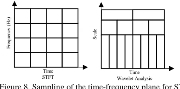
while the WT uses a self-adaptive window given by a wave-let function which duration changes within the frequency inversely related to the scale factor b (Giurgiutiu et al., 2003). This difference is illustrated by fig.8. When |b|>1, the wavelet is dilated and when |b|<1 the wavelet is compressed (Hammond & White,1996).
Figure 8. Sampling of the time-frequency plane for STFT and wavelet analysis.
There are multiple shapes of wavelets. The most popular is the Morlet wavelet :
2 0 /2 ² 1 i t s t sb b b t s e e a σ ω ψ − − − − = (7)
where ω0 is the central frequency of the mother wavelet
(modulation parameter) and σ is the scaling parameter that affects the width of the window.
In Nagaraju and Mallikarijuna Rao (2009), authors pro-posed the addition of phase angle information into 3D CWT plot to improve the crack detection in rotor systems. Moreo-ver, in Ozturk et al. (2008), authors proposed the extraction of the mean frequency from the scalogram to detect the progression of pitting damage in gears. It is important to note that the scalogram is defined as the squared modulus of the CWT which represents the energy of the signal in time-scale plane. In Rafiee and Tse (2009), authors proposed the autocorrelation of continuous wavelet coefficients for gear-box fault diagnosis instead of using the continuous wavelet coefficients (CWCs) themselves because they contain a lot of information in each scale that can generate a big loss of data after resampling. The autocorrelation of (CWC) over-comes this drawback by reducing the size of the data with keeping the content of information in each frequency band. Wang et al. (2010a) developed a fault growth parameter (FGP) for quantitative assessment based on the variation of complex Morlet CWT amplitude at all the scales of the transform under varying gearbox conditions. Authors pre-sented in Kankar et al. (2011) a method based on the mini-mum Shannon entropy criterion (MSEC) to choose the most convenient mother wavelet and to define the scale that matches the characteristic defect frequency. The adequate wavelet minimizes the Shannon entropy of the correspond-ing wavelet coefficients. Among all mother wavelets, the selected wavelet is the complex Morlet wavelet (CMW) and the results showed that it has satisfying results regarding bearing and gear fault detection. Lately, author proposed in Dai et al. (2016) a continuous wavelet transform approach for effective harmonic parameters estimation within the
detection and elimination of impulsive noise. In the context of PHM, recently, CWT was joined to a blind source separa-tion technique to analyze the wavelet coefficients and the evolution of each independent source is used for health assessment (Benkedjouh et al., 2018).
In order to increase the effectiveness of the EMD, it has been combined with the classic wavelet transform in Cao et al. (2016) and called the empirical wavelet transform (EWT). This method was applied for fault detection of the wheel-bearing of trains. To ensure the efficiency of this method, different faults were experimented (outer race fault, roller fault, and the compound fault of outer race and roller) and it showed satisfactory results.
3.3.2.Discrete wavelet transform
Another classical wavelet transform is the discrete wave-let transform (DWT). DWT uses instead of the continuous scale and time, discretized parameters to adapt the sampling condition of the physical signals : b=2j, s=k2j. Where j is the parameter about dilation, or the visibility in frequency and k is the parameter about the translation. This can be very powerful because it minimizes drastically the calculation time.
The DWT is expressed as follows:
( )
* 1 2 DWT( , ) ψ 2 2 j j j t k j k = x t − dt ∫
(8)This transform can be achieved by integrating a pair of low-pass and high-low-pass wavelet filters, respectively, h(k) and
g(k)=(−1)1-kh(1−k). These filters are obtained from the
wavelet function Ψ(t) and its scaling function Θ(t) given by (Mallat,1989):
( )
( )
( )
( )
( )
2 (2 ) ( ) 2 ( 2 with 0 2 ) k k k k t h k t k t g k t k h k g k Θ = Θ − Ψ = = = Θ − ∑
∑
∑
∑
(9)The coefficients h(k) are a sequence of real or complex numbers called the scaling function coefficients (or the scaling filter).
When applying these filters on the signal, low and high frequency elements are obtained:
( )
( )
1, ,
1, ,
(Low frequency elements) (High frequency element ) . s j k k k j j k k j k a h k d a g k a+ + = =
∑
∑
Where a and d are called respectively the approximation coefficient and the detail coefficient.
In Kim et al. (2007), a comparative study was applied on non-stationary vibration signals for fault detection of shaft-cracked during acceleration and deceleration. This study compared the STFT, WVD and DWT. The obtained results showed the efficiency of the DWT to extract good features.
Time STFT F re q u en cy (H z ) Time Wavelet Analysis S ca le
Moreover, to take into account the noisy state of the envi-ronment, authors developed in Omar and Gaouda (2012) a novel method to detect and localize gear tooth defects. This method uses the dynamic Kaiser’s window in the wavelet domain where the shape, size and sliding rate are variable. In Kumar and Singh (2013), authors underlined the difficul-ty to assess bearing fault size. So, they proposed the use of the Symlet wavelet to measure the width outer race defect of the roller bearing.
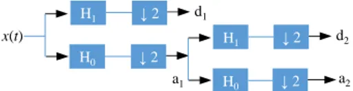
The combination of the WT with other techniques has been experimented in many works. For instance, a new data-driven method for fault detection in air handling units was developed in Yang and Nagarajaiah (2014). This method is based on the principal components analysis (PCA) and WT. The WT decomposes the signal in approximations and de-tails coefficients by passing the signal and the coefficients through low-pass H0 and high-pass H1 filters thanks to a
recursive algorithm. These coefficients are taken at different frequencies and the original signal at the kth step of decom-position is given by: x(t) = ak + dk + dk−1 +···+ d1 (see
fig.9).
Figure 9. Two level wavelet decomposition tree. where ↓2 denotes down sampling and means the number of coefficients is halved through the filters. The reconstitu-tion of the signal is done by filtering and up sampling (whi-tening the signal by filling with zeros between samples). The signal reconstructed must differentiate between faults and the perturbations which avoid false alarms. Features extracted from the reconstructed signal are injected in the PCA for fault detection.
3.3.3.Dual-tree complex wavelet transform
The WT technique has been used for signal denoising and undergoes improvements also like the case of Wang et al. (2010b). In this paper, authors proposed to use dual-tree complex wavelet transform (DTCWT) for the enhancement of signal denoising and multi-fault detection in rotating machines. DTCWT was introduced by Kingsbury (1998). It has properties that overcome some drawbacks of the DWT such as shift-invariance and the selection of direction which yields the possibility of using two or higher dimensions.
The complex analytical wavelet considers only positive frequency and is composed of two real-valued wavelets:
WC(t)=Wh(t)+jWg(t) where Wg(t)=H[Wh]. H[.] is the Hilbert
transform. Moreover, DTCWT is a combination of two parallel wavelet transforms which are represented by an upper and lower tree corresponding, respectively, to real and imaginary elements.
The DTCWT is almost shift invariant which means that it is possible to detect transient effects. Furthermore, it reduc-es frequency aliasing effects thanks to the property of ana-lytic filters.
In Wang et al. (2010b), the authors made a comparison between three techniques dedicated to denoising signal using the NeighCoeff shrinkage method. These methods are the DWT, the second generation wavelet transform (SGWT) and the DTCWT. The obtained results showed the efficien-cy of the DTCWT to diagnose composed faults of rolling elements bearing. First, the signal x(t) is transformed into the wavelet domain. The noisy wavelet coefficients are grouped and filtered with thresholding coefficients. The denoised signal is obtained using the inverse wavelet trans-form. The DTCWT has a small drawback which is the diffi-culty of multi-resolution analysis of fault characteristic data in high frequency band. This problem is resolved by using the dual tree complex wavelet packet transform (DTCWPT).
3.3.4.Wavelet packet transform
As a generalization of the DWT, the wavelet packet trans-form (WPT) was introduced for their better adaptability to non-stationary signals because it can perform an adaptive decomposition of the time-frequency axis (Serbes et al., 2016) and used, for instance, for signal processing of vibra-tion and acoustic emission signals. WPT is based on wavelet filters and the coefficients at each level can be written as:
( ) (
)
( ) (
)
2 1 2 1 1 * 2 * 2 K K j j K K j j W W n h n W W n g n + + + = − = − (10)whereWj2+K1 refers to the jth decomposed level of the wavelet packet coefficient at the frequency band of 2k (0 <k< 2j-1) with h(-2n) and g(-2n) are the low-pass and high-pass filters respectively which depend of the mother wave-let. Actually, the approximations and details are divided into small elements which increase the efficiency of WPT to-wards the CWT and DWT. The WPT is an efficient tool for analyzing the bearing fault signal in different frequency bands. This advantage was applied by Hemmati et al. (2016) for bearing fault detection. This method consists of calculat-ing the kurtosis-to-Shannon entropy ratio to determine the optimal mother wavelet and applying the WPT on the acoustic emission signals of roller bearing. After this, the envelope of acoustic emission signals is applied in the dif-ferent frequency bands given by the WPT and the Kurtosis-to-Shannon entropy ratio is calculated for each envelope in order to determine the optimal frequency band given by the highest ratio and then the lowest Shannon entropy value. Then, this band pass is de-noised using adaptive threshold-ing method given by thr= 2 ln( )× n ×s where n is the length of the discrete signal and s is an estimate of the noise level. Finally, the spectrum of squared Hilbert transform is applied under variable rotating speeds and loading condi-tions to estimate the time difference between the double acoustic emission impulses for estimating the defect size on rolling element bearings.
3.3.5.Second generation wavelet transform
Another technique derived from the DWT is the second generation wavelet transform (SGWT) where the wavelets
H1 ↓ 2 d1 H0 ↓ 2 H1 ↓ 2 d2 H0 ↓ 2 x(t) a2 a1
functions are not designed by translations and dilations of the mother wavelet but designed by applying a lifting scheme (Sweldens, 1998). In an analogous way to the DWT, the lifting scheme aims, firstly, at decomposing the signal into approximation and detail coefficients. This can be achieved by, firstly, splitting the signal into odd and even components where:
( )
( )
(
{
(
)
}
{
( )
}
)
(
)
( )
2 1 , 2 { 2 1 } { 2 } odd even split x t x t x t x x t x x t = − = − = (11)with t=1,2,…,n. Secondly, the detail coefficients are given by D = xodd -Predict (xeven) where Predict(xeven) is a
predic-tion operator of adjacent even components. The predicpredic-tion operator can be an average of two even indexed neighbors. In the same way, the approximation coefficients are given by A = xeven+ Update (detail) where Update (detail) is an
update operator based on previously calculated coefficients. The P and U operators are analogous to g and h functions used for the DWT.
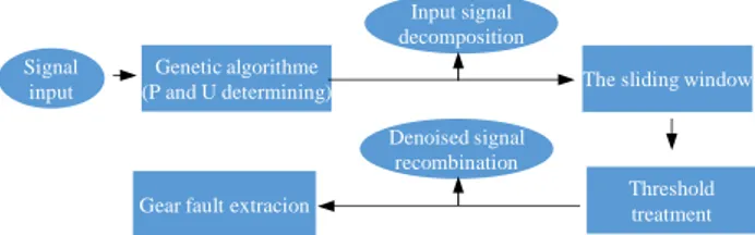
Many researches presented some enhancement on the SGWT. For instance, authors presented in Yuan et al. (2010) a novel method (see fig.10) for gear fault detection. This method consists of combining customized multiwave-let schemes to a sliding window denoising. First, different vector prediction and update operators with the desirable properties of biorthogonality, symmetry, short support and vanishing moments are built, by using Hermite spline inter-polation (Averbuch & Zheludev, 2002). Then, the adequate operators are chosen based on the minimum entropy prin-ciple. Then, by considering the period nature of the gearbox signals, a multiwavelet sliding window is used to divide the detail signal in segmentations to keep significant informa-tion which leads to extract the fault features for fault identi-fication in gearbox signals. These segmentations undergo a threshold denoising. Then the denoised signal is recon-structed.
Figure 10. The flow chart of the proposed method. Wavelet transform performs as band pass filtering with a constant relative-bandwidth. This is suitable to analyze some signals but restricts the adaptability of the transform. To deal with more general situations, Mallat and Zhang (1993) proposed the matching pursuit algorithm and the concept of time-frequency atoms. In fact, to extract informa-tion from a signal, it may be interesting to decompose this signal into a family of well-localized functions both in time and in frequency. These functions, called "time-frequency" atoms, are grouped in a dictionary. Mallat and Zhang pro-pose to generate such a dictionary by modifying the scale,
by translating and modulating a simple window g(t) ϵ L²(ℝ). Consider the scale b > 0 , the frequency modulation f0 and
the translation s. We note γ= (b, s, f0) ϵ Γ =ℝ+×ℝ2 and we
define a "time-frequency" atom as follows:
0 1 ( ) t s if t g t g e b b γ − = (12)
Figure 11. Representation of the energy of an atom "time-frequency" according to the scale b, the frequency
modula-tion f0 and the translation s. As shown in figure 11:
- In comparison with the time, the function gγ(t) is centered
around s and its energy is concentrated near s with a size proportional to b.
- In comparison with the frequency, the Fourier transform
gγ(ω) is centered around f0 and its energy concentrated near ξ with a size proportional to 1/b.
The resulting dictionary is the family of vectors D = (gγ(t))γ∈Γ. The dictionary is complete only if the linear
com-bination of the vectors of D is dense in the Hilbert space, here L2 (ℝ).
To effectively represent a signal x(t), we must select an appropriate subset of atoms (gγn(t)) n∈N with γn = (bn, sn, f0n)
such as : ( ) n( n( )) n x t a gγ t +∞ =−∞ =
∑
(13)The coefficients an depend on the atom gγn(t) chosen. The
selected atoms and their corresponding coefficients provide the information about the time-frequency characteristics of the signal. This approach was proposed in the paper of Liu et al. (2002) to detect bearing failure. The vibration signal is first decomposed into time-frequency atoms with matching pursuit. Then, the vibration signature was ex-tracted using high frequency atoms with small scales. Since the signature obtained this way contained less unrelated components to the defects than traditional band-pass filter-ing, it thus had a higher signal-to-noise ratio and gave more explicit information for the bearing failure detection.
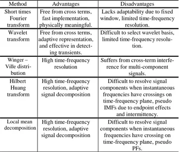
Table 4 allows distinguishing two types of time-frequency representation: linear (WT, STFT) and quadratic (Wigner Ville distribution, HHT). The latter are more effi-cient than the first in terms of time-frequency resolution. On the other hand, they suffer from problems of interference between frequency components.
Signal input Genetic algorithme (P and U determining) Input signal decomposition
The sliding window
Threshold treatment Denoised signal
recombination Gear fault extracion
b Frequency Time 1/b f0 s 0 energy of an atom "time-frequency"
Method Advantages Disadvantages Short times
Fourier transform
Free from cross terms, fast implementation, physically meaningful.
Lacks adaptability due to fixed window, limited time-frequency
resolution. Wavelet
transform
Free from cross terms, adaptive representation,
and effective in detect-ing transients.
Difficult to select wavelet basis, limited time-frequency
resolu-tion. Winger – Ville distri-bution High time-frequency resolution
Suffers from cross-term interfe-rence for multi-component
signals. Hilbert Huang transform High time-frequency resolution, adaptive signal decomposition
Difficult to resolve signal components when instantaneous
frequencies have crossings on time-frequency plane, pseudo IMFs due to endpoint effects
and intermittency. Local mean decomposition High time-frequency resolution, adaptive signal decomposition
Difficult to resolve signal components when instantaneous
frequencies have crossing on time-frequency plane, pseudo
PFs.
Table 4. Categories of time-frequency analysis methods
4. CONCLUSION
This paper reviews different signal processing techniques used to extract indicators for bearings and gearboxes. The importance of these mechanical elements in the industry and their criticality leads to unfortunate consequences (mainten-ance costs, safety, etc.) and thus justifies the need of effec-tive fault indicators. Techniques currently used are based on the use of statistical indicators such as the RMS and the Kurtosis. These indicators give good results for estimating the general degradation of the system but find their limits to locate the fault responsible of the degradation. The spectral analysis allows highlighting the characteristic frequencies of faults. In contrast to time-frequency techniques, spectral analysis does not take into account the “time” information. In other words, the presence of a frequency component can be detected but no information on the time occurrence is available. Fourier transform and the cepstral analysis are the most commonly used for stationary signals. The time-frequency analysis makes possible the representation on the same plane temporal and frequency characteristics when the signals are non-stationary and when information about the frequency bands where the defects can appear are available. All the proposed signal processing techniques can be classified as follows: time analysis, Fourier analysis, cep-stral analysis, the cyclostationarity analysis, envelope analy-sis and time-frequency analyanaly-sis. These methods are now available in any modern spectrum analyzer but not very well applied in the industry. The results obtained by these tech-niques in the references discussed in this paper have contri-buted positively to choose among them the one that will define a framework for industrials to monitor bearings and gearboxes.
REFERENCES
Antoni, Jerome & Randall, R.B. (2002). Differential Diag-nosis of Gear and Bearing Faults. Journal of Vibration
and Acoustics. 124(2): 165-171.
Ali, J. B., Fnaiech, N., Saidi, L., Chebel-Morello, B., and Fnaiech, F. (2015). Application of empirical mode de-composition and artificial neural network for automatic bearing fault diagnosis based on vibration signals.
Ap-plied Acoustics, 89:16 – 27.
Appleby, M. P. (2003). Wear debris detection and oil analy-sis using ultrasonic and capacitance measurements. Mas-ter’s thesis, Master of Science Thesis, the Graduate Fa-culty of the University of Akron.
Auger, F. and Flandrin, P. (1996). Ctime-frequency toolbox.
CNRS France-Rice University, 46 (1996).
Averbuch, A. Z. and Zheludev, V. A. (2002). Lifting scheme for biorthogonal multiwavelets originated from
hermite splines. IEEE Transactions on Signal
Processing, 50(3):487–500.
Barszcz, T. and Jablonski, A. (2011). A novel method for the optimal band selection for vibration signal demodu-lation and comparison with the kurtogram. Mechanical
Systems and Signal Processing, 25(1):431 – 451.
Bellini, A., Immovilli, F., Rubini, R., and Tassoni, C. (2008). Diagnosis of bearing faults of induction ma-chines by vibration or current signals: A critical compar-ison. In IEEE Industry Applications Society Annual
Meeting, pages 1–8.
Bengtsson, M. (2003). Standardization issues in condition based maintenance. In Condition Monitoring and
Diag-nostic Engineering Management, pages 651–660.
Bennett, W. R. (1958). Statistics of regenerative digital
transmission. Bell System Technical Journal,
37(6):1501–1542.
Benkedjouh, T., Zerhouni, N., & Rechak, S. (2018). Tool wear condition monitoring based on continuous wavelet transform and blind source separation. The
Internation-al JournInternation-al of Advanced Manufacturing Technology,
1-13.
Bleakie, A., & Djurdjanovic, D. (2013). Feature extraction, condition monitoring, and fault modeling in semicon-ductor manufacturing systems. Computers in
Indus-try, 64(3), 203-213.
Bonnardot, F. (2004). Comparison between angular and
time domain analysis of rotating machine vibratory sig-nals. Study of fuzzy-cyclostationnarity concept. PhD
the-sis, Institut National Polytechnique de Grenoble - INPG. Burgess, L. and Shimbel, T. (1995). What is the prognosis
on your maintenance program. In Engineering and
Min-ing Journal, volume 196, pages 32–35.
Cao, H., Fan, F., Zhou, K., and He, Z. (2016). Wheel-bearing fault diagnosis of trains using empirical wavelet transform. Measurement, 82:439 – 449.
Casoli, P., Bedotti, A., Campanini, F., & Pastori, M. (2018). A Methodology Based on Cyclostationary Analysis for
Fault Detection of Hydraulic Axial Piston
Chen, K., Li, X., Wang, F., Wang, T., and Wu, C. (2012). Bearing fault diagnosis using wavelet analysis. In
Inter-national Conference on Quality, Reliability, Risk, Main-tenance, and Safety Engineering, pages 699–702.
Dai, Y., Xue, Y., and Zhang, J. (2016). A continuous wave-let transform approach for harmonic parameters estima-tion in the presence of impulsive noise. Journal of Sound
and Vibration, 360:300 – 314.
Didier, G. (2004). Modélisation et diagnostic de la machine
asynchrone en présence de défaillances. PhD thesis,
Un-iversité Nancy 1, France.
Do, V. T. and Chong, U.-P. (2011). Signal model-based fault detection and diagnosis for induction motors using features of vibration signal in two- dimension domain.
Journal of Mechanical Engineering, 57(9):655–666.
Dron, J. P., Bolaers, F., Rasolofondraibe, I. (2004). Im-provement of the sensitivity of the scalar indicators (crest factor, kurtosis) using a de-noising method by spectral subtraction: application to the detection of de-fects in ball bearings. Journal of Sound and
Vibra-tion, 270(1-2), 61-73.
El Badaoui, M. (1999). Contribution to the Vibratory
Diag-nosis of the Complex gears by the Cepstrum analysis.
Theses, Université Jean Monnet - Saint-Etienne.
Elghazel, W., Bahi, J., Guyeux, C., Hakem, M., Medjaher, K., and Zerhouni, N. (2015). Dependability of wireless sensor networks for industrial prognostics and health management. Computers in Industry, 68:1 – 15.
Feng, Z. and Liang, M. (2014). Fault diagnosis of wind turbine planetary gearbox under nonstationary condi-tions via adaptive optimal kernel time-frequency analy-sis. Renewable Energy, 66:468 – 477.
Feng, K., Wang, K., Zhang, M., Ni, Q., & Zuo, M. J. (2017). A diagnostic signal selection scheme for plane-tary gearbox vibration monitoring under non-stationary operational conditions. Measurement Science and
Technology, 28(3), 035003.
Franklin, G. F., Da Powell, J., & Emami-Naeini, A. (2010) Feedback Control of Dynamic Systems (6th).
Giurgiutiu, Victor, and Yu, L. (2003). In Comparison of
Short-time Fourier Transform and Wavelet Transform of Transient and Tone Burst Wave Propagation Signals For Structural Health Monitoring, pages 1267–1274.
Gong, X. and Qiao, W. (2013). Bearing fault diagnosis for direct-drive wind turbines via current-demodulated sig-nals. IEEE Transactions on Industrial Electronics, 60(8):3419–3428.
Hammond, J. and White, P. (1996). The analysis of non-stationary signals using time-frequency methods.
Jour-nal of Sound and Vibration, 190(3):419 – 447.
Han, J., Dong, F., and Xu, Y. Y. (2009). Entropy feature extraction on flow pattern of gas/liquid two-phase flow based on cross-section measurement. Journal of Physics:
Conference Series, 147(1):012041.
Hemmati, F., Orfali, W., and Gadala, M. S. (2016). Roller bearing acoustic signature extraction by wavelet packet
transform, applications in fault detection and size esti-mation. Applied Acoustics, 104:101 – 118.
Heng, A., Zhang, S., Tan, A. C., and Mathew, J. (2009). Rotating machinery prognostics: State of the art, chal-lenges and opportunities. Mechanical Systems and
Sig-nal Processing, 23(3):724 – 739.
Holmberg, K., Adgar, A., Arnaiz, A., Jantunen, E., Masco-lo, J., and Mekid, S. (2010). E-maintenance. Springer Publishing Company, Incorporated, 1st edition.
Holroyd, T. J. (2005). The application of ae in condition monitoring. In International Conference on Condition
Monitoring, volume 47, pages 481–485.
Hong, L. and Dhupia, J. S. (2014). A time domain approach to diagnose gearbox fault based on measured vibration signals. Journal of Sound and Vibration, 333(7):2164 – 2180.
Hountalas, D. T. (2000). Prediction of marine diesel engine performance under fault conditions. Applied Thermal
Engineering, 20(18):1753 – 1783.
Jaloretto, M. R., de Oliveira, C. R. E., and Kawakami, R. (2009). Trend analysis for prognostics and health moni-toring. In CTA-DLR Workshop on Data Analysis &
Flight Contr, pages 14–16.
Kalgren, P. W., Byington, C. S., Roemer, M. J., and Wat-son, M. J. (2006). Defining phm, a lexical evolution of maintenance and logistics. In IEEE Autotestcon, pages 353–358.
Kankar, P., Sharma, S. C., and Harsha, S. (2011). Rolling element bearing fault diagnosis using wavelet transform.
Neurocomputing, 74(10):1638 – 1645.
Kar, C. and Mohanty, A. (2006). Monitoring gear vibrations through motor current signature analysis and wavelet transform. Mechanical Systems and Signal Processing, 20(1):158 – 187.
Kim, B., Lee, S., Lee, M., Ni, J., Song, J., and Lee, C. (2007). A comparative study on damage detection in speed-up and coast-down process of grinding spindle-typed rotor-bearing system. Journal of Materials
Processing Technology, 187-188:30 – 36.
Kim, N. H., An, D., & Choi, J. H. (2017). Prognostics and
health management of engineering
sys-tems. Switzerland: Springer International Publishing. Kingsbury, N. (1998). The dual-tree complex wavelet
trans-form: A new technique for shift invariance and direc-tional filters. 8th IEEE DSP Workshop, pages 319–322. Kumar, R. and Singh, M. (2013). Outer race defect width
measurement in taper roller bearing using discrete wave-let transform of vibration signal. Measurement, 46(1):537 – 545.
Kumar, S., Dolev, E., and Pecht, M. (2010). Parameter se-lection for health monitoring of electronic products.
Mi-croelectronics Reliability, 50(2):161 – 168.
Laerhoven, K. V., Aidoo, K. A., and Lowette, S. (2001). Real-time analysis of data from many sensors with neur-al networks. In Proceedings Fifth Internationneur-al
Sympo-sium on Wearable Computers, pages 115–122.
Lee, J.-Y. (2013). Sound and vibration signal analysis using improved short-time fourier representation. International