To cite this version
Tanguy, Sébastien and Sagan, Michael and
Lalanne, Benjamin and Couderc, Frédéric and Colin, Catherine
Benchmarks and numerical methods for the simulation of boiling
flows. (2014) Journal of Computational Physics, vol. 264 . pp. 1-22.
ISSN 0021-9991
O
pen
A
rchive
T
OULOUSE
A
rchive
O
uverte (
OATAO
)
OATAO is an open access repository that collects the work of Toulouse researchers and
makes it freely available over the web where possible.
This is an author-deposited version published in :
http://oatao.univ-toulouse.fr/
Eprints ID : 11191
To link to this article :
DOI: 10.1016/j.jcp.2014.01.014
http://dx.doi.org/10.1016/j.jcp.2014.01.014
Any correspondance concerning this service should be sent to the repository
administrator:
[email protected]
Benchmarks and numerical methods for the simulation of
boiling flows
Sébastien Tanguy
a,
∗
, Michaël Sagan
a, Benjamin Lalanne
a, Frédéric Couderc
b,
Catherine Colin
aaIMFT CNRS UMR 5502, Université de Toulouse, France bIMT CNRS UMR 5219, Université de Toulouse, France
a b s t r a c t
Keywords: Level set Ghost Fluid Method Two-phase flows Boiling flows Phase change Jump conditions
Comparisons of different numerical methods suited to the simulations of phase changes are presented in the framework of interface capturing computations on structured fixed computational grids. Due to analytical solutions, we define some reference test-cases that every numerical technique devoted to phase change should succeed. Realistic physical properties imply some drastic interface jump conditions on the normal velocity or on the thermal flux. The efficiencies of Ghost Fluid and Delta Function Methods are compared to compute the normal velocity jump condition. Next, we demonstrate that high order extrapolation methods on the thermal field allow performing accurate and robust simulations for a thermally controlled bubble growth. Finally, some simulations of the growth of a rising bubble are presented, both for a spherical bubble and a deformed bubble.
1. Introduction
Boiling flow is a topic of interest for various industrial applications as spray cooling, heat exchanger, cryogenic applica-tions or fluid storage in micro-gravity for spatial applicaapplica-tions. The development of numerical techniques dedicated to the direct numerical simulation of boiling flow is still challenging. A preliminary step, to compare these simulations with large scale experiments, is to succeed some benchmarks for simplified configurations. Accurate benchmarks, involving analytical theories, allow studying the performances of different numerical methods. This is relevant in the difficult context of direct numerical simulation of two-phase flows when phase changes occur. One of the main objectives of this paper is to propose a methodology in order to validate and to assess the global accuracy of numerical methods relevant for the simulations of boiling flows.
In[29]and[15], the authors present pioneering works where new numerical methods are designed to compute boiling flows respectively with a Level Set Method and with a Front Tracking algorithm for the interface description. In [17,37], the authors developed numerical methods to compute boiling flows with the Volume Of Fluid method. Some attempts of boiling flows simulations with Second Gradient Method have been proposed in [13]. In[38], computations with high density ratio are presented with a sharp-interface marker points method. A general methodology is presented in [3–5]
for 3D computations in complex geometries. The coupled Level Set – Volume Of Fluid method is applied to boiling flows in [35]. A new approach, with a subgrid scale treatment of boundary layers, is proposed in [7,8] to deal with impacting boiling droplets on hot walls. In [30,31], 3D computations of the nucleate boiling on a horizontal surface and saturated
*
Corresponding author. Tel.: +33 5 34 32 28 08; fax: +33 5 34 32 28 99. E-mail address:[email protected](S. Tanguy).film boiling on a horizontal cylinder are presented. In[11,34], the authors use the Ghost Fluid Method to design a sharp interface method devoted respectively to boiling flows and to droplets vaporization. More recently, sharp interface numerical methods for boiling flows have also been designed in the context of the Front Tracking method[26]. Few of the works cited above propose accurate comparisons of multidimensional computations with analytical theories, as it has been done with a boundary-fitted method in [19]. The accuracy and the performances of these various numerical methods are therefore difficult to evaluate. It will be demonstrated in this article, that the way to compute the boiling mass flow rate has a strong influence on the global accuracy. Another sensitive issue concerns the computation of the expansion flow due to the phase change of the liquid into a vapor (or collapsing flow for condensation). It will be shown in this paper that the Continuous Surface Force approach, where the interfacial source terms are smoothed across interface, can fail to determine accurately the bubble expansion rate due to the smearing out of the velocity field at the interface. At the opposite, we provide numerical evidences that a sharp interface method, as the Ghost Fluid Method, succeeds to compute the bubble expansion rate.
Our main focus is the numerical simulation of the bubble growth in a superheated liquid. In that specific situation, when the bubble is static, an analytical bubble growth prediction can be determined according to Scriven[28]. Bubble growth rate depends on thermal boundary layer thickness in the liquid around the bubble. It can be shown from theoretical analysis that the dimensionless bubble growth rate depends on the Jakob number Ja and a dimensionless parameter
ε
function of the density ratio between the vapor and the liquid. This analytical theory is very attractive to design benchmarks for boiling flows. A particular attention shall be paid to high Jakob number simulations (about 10) when the thermal boundary layer around the bubble is very thin in comparison to the bubble diameter. Performing simulations on this configuration involves very drastic resolution conditions which are particularly suitable to assess the global accuracy of the method. Another important requirement of this work is to design a numerical method whose accuracy and stability properties are preserved whatever the density ratio between the vapor and the liquid. Indeed, it is well known that strong density ratio and strong capillary effects can damage stability and accuracy properties of numerical methods, and that problem is even more acute if a phase change occurs. So the simulations presented in this paper imply strong discontinuities at the interface, as for liquid/vapor water which involves a density ratio above 1600 at ambient pressure conditions.2. Equations and jump conditions
The model used to deal with a phase change is identical to those from[11], where the liquid and the gas are supposed incompressible and monocomponent. We assume the boiling temperature is uniform and only depends on the external pres-sure. Thus, the Marangoni convection, resulting from boiling temperature variation, cannot occur in that situation. Moreover, considering low Mach number flows with low temperature variations in the vapor phase as well as in the liquid phase, we can expect that the velocity field will respect divergence-free condition (except at the interface when phase changes occur). A simplified energy conservation equation, based on enthalpy formulation, is used to predict temperature variations in the two phases. In this equation, the viscous heating and pressure effects are neglected.
The governing equations can be formulated in a “Whole-Domain Formulation”[2,18,32,36]or in a “Jump Condition Form”
[16,24]. These two formulations, theoretically equivalent, imply different numerical methods when dealing with discontin-uous fields. We define N as the normal vector at an interface
E
Γ
pointing in the direction of vapor phase, and the jump conditions at the interfaceΓ
are expressed with the following operator:[
f]
Γ=
fvap−
fliq2.1. Mass conservation equation
Both the liquid and the vapor phases are considered incompressible. So the divergence-free property is imposed in the bulk of the two phases:
∇ · E
V=
0 (1)where V is the velocity vector of the fluid flow. At the interface, if phase changes occur, the following velocity jump
E
condition must be respected to preserve the mass conservation:
[ E
V]
Γ= ˙
m·
1ρ
¸
ΓE
N (2)where m is the phase change local mass flow rate and
˙
ρ
is the density of the considered phase. The field equations are written in each phase separately and additional jump conditions have to be imposed at the interface to respect the conservation of mass, momentum and energy. This is known as the Jump Condition Formulation[27].An equivalent formulation can be favored to express the mass conservation by using a Dirac distribution at the interface. The jump conditions are expressed in the field equations by introducing singular source terms:
∇ · E
V= ˙
m·
1ρ
¸
Γδ
Γ (3)where
δ
Γ is a Dirac distribution equal to zero everywhere in the field, except at the interface. The main difficulty of thisformulation, commonly known as the Whole Domain Formulation[27], lies in the definition of an accurate discretization of singular source terms. One of the most common mean consists in smearing out the interface across 2 or 3 computational cells by defining a smoothed Heaviside or Dirac Function. This is the so-called Continuum Surface Force approach[2,32,36], which is very widespread to compute the surface tension force when solving the Navier–Stokes equations.
2.2. Momentum balance
For incompressible flows and Newtonian fluids, the momentum balance leads to the Navier–Stokes equation which can be expressed in a non-conservative form as follows:
ρ
µ ∂ E
V∂
t+ E
V· ∇ E
V
= −∇
p+
µ
∇
2VE
+
ρ
E
g (4)where p designs the pressure field,
µ
is the dynamic viscosity of the considered phase, andE
g is the gravity acceleration.The pressure must respect the following jump condition[11,12]:
[
p]
Γ=
σ κ
+
2·
µ
∂
VN∂
N¸
Γ−
·
1ρ
¸
Γ˙
m2 (5)with
σ
the surface tension,κ
the local interface curvature and∂VN∂N the normal derivative of the normal velocity component. The first term of the right hand side of Eq.(5)models capillary effects, the second term is a jump condition on the normal viscous stress, and the third term is the recoiling pressure occurring with phase change.
Otherwise, when dealing with a Whole Domain Formulation, the capillary effects are integrated in the momentum balance equation by adding a singular term[2,32,36]:
ρ
µ ∂ E
V∂
t+ E
V· ∇ E
V
= −∇
p+ ∇ · (
2µ
D)
−
σ κ
NE
δ
Γ+
ρ
E
g (6)with D
=
∇ EV+∇2 TVE the deformation tensor. The density and viscosity can be expressed as follows:ρ
=
ρ
liq+ (
ρ
vap−
ρ
liq)
HΓ (7)µ
=
µ
liq+ (
µ
vap−
µ
liq)
HΓ (8)HΓ is a Heaviside distribution, equal to 1 in the liquid phase and equal to 0 in the vapor phase.
2.3. Energy conservation equation
The energy conservation equation can be formulated with different primitive variables as the internal energy or the enthalpy. The internal energy is favored to describe thermodynamics phenomena in closed systems, and the enthalpy is more commonly used for description of quasi-isobaric phenomena (usually open systems). This study deals with isobaric phenomena which only imply weak pressure gradients due to dynamical effects. Thus, the following equation to describe energy conservation, resulting of an enthalpy primitive variable formulation, is well suited to our problem:
ρ
Cpµ ∂
T∂
t+ E
V· ∇
T
= ∇ · (
k∇
T)
(9)where Cp is the heat capacity per unit of mass at constant pressure, and k is the thermal conductivity. When phase changes occur, an additional jump condition must be imposed on the thermal flux:
[−
k∇
T· E
N]
Γ= − ˙
m¡
Lvap
+ (
Cpliq−
Cpvap)(
Tsat−
Tint)
¢
(10)
with Lvap the latent heat of vaporization, Tsat the saturation temperature associated to the considered pressure, and Tint the local interface temperature. Usually, it can be deduced from arguments about the interface entropy condition that the temperature is continuous at the interface [12]. However, considering additional physical effects as the variation of temperature saturation due to the pressure jump condition and the interface thermal resistance due to molecular effects, some corrections to that assumption can be provided, see [15]for a more detailed study on that point. In this work, we suppose the interface temperature is always continuous and equal to the saturation temperature which is supposed uniform (mono-component vapor phase and liquid phase) and constant (isobaric approximation).
As for the mass conservation equation and the momentum equation, the Whole Domain Formulation can be applied to the energy conservation equation to include the latent heat effect as a singular term [15], leading to the following expression:
ρ
Cpµ ∂
T∂
t+
V· ∇
T
2.4. Level set methods and interface description
The interface motion is captured with a Level Set Method[6,22,32]. It consists in solving a convection equation for a Level Set Function
ϕ
, which zero level curve separates the vapor field (ϕ
>
0) from the liquid field (ϕ
<
0):∂φ
∂
t+ E
Vint· ∇φ =
0 (12)with V
E
int the interface velocity. Whereas this velocity has a physical meaning only at the interface, it is worth noting it should be continuously extended away from the interface in order to solve Eq.(12)with a regular velocity field. If no phase change occurs, the interface velocity is equal to the fluid velocity on the interface. In this situation, the fluid velocity is continuous, so there is no doubt about the choice of the interface velocity. Otherwise, if phase changes occur, the interface velocity has to be computed with one of the two following relations[11]:E
Vint= E
Vvap−
˙
mρ
vapE
N= E
Vliq−
˙
mρ
liqE
N (13)An important feature of a numerical method lies in its ability to clearly make out the vapor velocity field from the liquid velocity field, and to avoid transporting the interface with a fictitious velocity field. To do that, one of the two expressions of Eq.(13)must be expressly chosen to compute the interface velocity. That can be done quite naturally in the framework of the Ghost Fluid Method[6,11,16,21]. Next, a reinitialization step[32]must be achieved to ensure the
ϕ
function remains a signed distance in the computation domain. It can be done by solving iteratively the specific PDE:∂φ
∂
τ
=
sign(φ
0)
¡
1
− |∇φ|
¢
(14)
with
ϕ
the reinitialized distance function,τ
a fictitious redistancing time and sign(ϕ
0) is a smoothed signed function defined in[16,32]. By preserving the signed distance function property in the interface neighborhood, a good accuracy is maintained when computing the interface geometrical properties as normal vector or curvature, with the following simple relations:E
N
=
∇φ
|∇φ|
,
κ
(φ)
= −∇ · E
N (15)3. Numerical methods
In the framework of the direct numerical simulation of boiling flow, further numerical issues must be overcome due to the interface propagation and the discretization of discontinuous fields. Numerical tools must be developed to deal with the normal velocity jump condition, to determine accurately the thermal field close to the interface and to deduce the boiling mass flow rate. The objectives of this paper are both to propose some benchmarks using theoretical solutions, and to do a parametrical and comparative study between different extrapolation methods.
All convective derivatives in Eqs.(4),(9),(12),(14)are computed using a fifth order WENO scheme[14]. Diffusion terms in Eqs.(4),(9)are computed with a central second order scheme.
3.1. Coupling the mass conservation and the Navier–Stokes resolution with appropriate jump conditions
First works on the direct numerical simulation of boiling flows have used a smoothed Dirac function in the right hand side of the continuity equation, Eq.(3), to compute the motion expansion of the fluid due to the phase change of a heavy fluid (liquid) in a light fluid (vapor). Some examples can be found in[15,29,37]. A projection method for the temporal discretization of the Navier–Stokes equations leads to the following algorithm for solving Eqs.(3)and(6):
E
V∗= E
Vn− 1
tµ
E
Vn· ∇ E
Vn−
∇ · (
2µ
D n)
ρ
n+1+
σ κ
NE
δ
ε(φ)
ρ
n+1− E
g
(16)∇ ·
µ
∇
pn+1ρ
n+1
=
∇ · E
1
Vt ∗− ˙
m·
1ρ
¸
Γδ
ε(φ)
(17)E
Vn+1= E
V∗− 1
t∇
p n+1ρ
n+1 (18)where the Dirac distribution can be approximated by a smoothed function
δ
ε(φ)
[31,32]:δ
ε(φ)
=
0 ifφ <
−
ε
1 2ε(
1+
cos(
πφ ε))
if|φ| 6
ε
0 ifφ >
ε
(19)The smoothing of a Dirac distribution introduces a fictitious interface thickness 2
ε
=
31x where1
x is the length of acomputational cell.
Otherwise, in the framework of the Jump Condition Formulation, a numerical method has been proposed in [21] to impose the normal velocity jump condition at the interface, preserving the interface sharpness by defining ghost cells for the velocity field. This method, initially developed for the propagation of flame fronts, has been used for boiling flows in
[11] and modified in[34]to improve the temporal evolution of the mass prediction when dealing with a vaporizing liquid drop. It consists in defining an extension of the velocity field:
If
ϕ
>
0: E
Vliqghost= E
Vvapn− ˙
mn·
1ρ
¸
ΓE
N (20a)If
ϕ
<
0: E
Vvapghost= E
Vliqn+ ˙
m n·
1ρ
¸
ΓE
N (20b)Next, the prediction step of a projection method requires to compute an intermediate velocity field:
E
Vliq∗= E
Vliqn− 1
tµ
E
Vnliq· ∇ E
Vliqn−
∇ · (
2µ
D n liq)
ρ
n+1− E
g
(21a)E
Vvap∗= E
Vnvap− 1
tµ
E
Vvapn· ∇ E
Vvapn−
∇ · (
2µ
D n vap)
ρ
n+1− E
g
(21b)We use the discretization of viscous tensor described in [33]. This discretization is close to the original discretization of viscous terms firstly developed for the Delta Function Method[32], except for the interface sharpness which is preserved by using a harmonic average to compute the viscosity on the boundary of the cells which are crossed by the interface. This method is suited to deal with phase changes, unlike the one presented in the original paper on the Ghost Fluid Method for incompressible flows[16]. Moreover, its implementation is easier.
The second step of the projection method consists in determining the pressure field:
If
ϕ
<
0: ∇ ·
µ
∇
pn+1ρ
n+1
=
∇ · E
V ∗ liq1
t (22a) Else ifϕ
>
0: ∇ ·
µ
∇
pn+1ρ
n+1
=
∇ · E
V ∗ vap1
t (22b)Following the sharp interface method defined in [16,20,33], the surface tension effects and the density jump are included when Eqs. (22a)and(22b)are solved simultaneously. Next, the final velocity field can be determined with the following correction step:
E
Vliqn+1= E
Vliq∗− 1
t∇
p n+1ρ
n+1 (23a)E
Vvapn+1= E
Vvap∗− 1
t∇
p n+1ρ
n+1 (23b)From the final correction step, Eqs.(20a)and(20b)can be applied to start the next time step. In[34], the authors propose a more complex velocity field extension to improve the mass evolution prediction for vaporizing droplets. It consists in building a divergence-free velocity field extension, for the fluid velocity field used to transport the interface in Eqs.(12)
and(13). Unlike[34], in this work, the interface is transported with the vapor phase velocity field. This extension consists in computing a ghost pressure field by solving a Poisson equation:
∇ ·
µ
∇
pghostρ
n+1
=
∇ · E
V ∗ vap1
t (24)and to define the following velocity field extension which respects the divergence-free property for the vapor velocity field:
If
ϕ
>
0: E
Vliqghost= E
Vvapn+1− ˙
m·
1ρ
¸
ΓE
N (25a)If
ϕ
<
0: E
Vvapghost= E
Vvap∗− 1
t∇
pghost
3.2. Solving the energy conservation equation with appropriate Dirichlet boundary conditions
Using, the same procedure as in[11], the thermal field is computed separately in the liquid domain and in the vapor domain with the following elementary first order semi-implicit time discretization:
If
ϕ
<
0:
ρ
liqCpliqTn+1− 1
t∇ ·
¡
kliq
∇
Tn+1¢ =
ρ
liqCpliq¡
Tnliq
− 1
tVE
liq· ∇
Tnliq¢
(26a) If
ϕ
>
0:
ρ
vapCpvapTn+1− 1
t∇ ·
¡
kvap∇
Tn+1¢ =
ρ
vapCpvap¡
Tvapn− 1
tVE
vap· ∇
Tvapn¢
(26b)
A uniform Dirichlet condition on the temperature is imposed at the interface for the two domains, to ensure the interface temperature is equal to the saturation temperature. This condition is computed using a second order discretization proposed in[9]. An attractive feature of this second order discretization is to preserve a symmetric definite positive matrix allowing the use of standard Black-Box solver (Incomplete Cholesky Conjugate Gradient). This method has also been applied in[34]
to solve the mass fraction evolution for the droplet vaporization of a pure liquid in a two-component vapor phase. All the computations presented in this paper use this second order discretization for the thermal field. Let us notice that, higher order discretization for an interface Dirichlet boundary condition has been proposed in[10]. But their application does not seem currently relevant in the more complex framework of boiling flows. Recently, a second order finite volume discretization for an embedded boundary condition at the interface has been developed in[23]. This attractive method also preserves the matrix symmetry and allows working with Neumann or Robin boundary conditions.
3.3. Temperature field extrapolation
As for the velocity field, the extrapolation of the temperature field in each side of the interface must be performed to populate ghost cells. In[6], an extrapolation technique, based on a PDE resolution, is proposed to construct a continuous extension of a discontinuous variable following the normal direction at the interface. It consists in solving iteratively a hyperbolic equation, for the extended variable f in the ghost domain:
∂
f∂
τ
± E
N· ∇
f=
0 (27)Improvements of this technique have been proposed in[1], to construct an extrapolated field that preserves the continu-ity of normal derivatives. It can be done by solving one additional PDE to impose the first derivative continucontinu-ity (linear extrapolation), two additional PDE to impose the first and the second derivatives continuity (quadratic extrapolation), and
n additional PDE to impose the continuity until the n-order derivative. Considering the thermal field computation is
sec-ond order, our numerical investigations have been limited to linear and quadratic extrapolations. It leads to the successive resolution of the 3 following PDE for the extension of the temperature field in the liquid domain:
∂
Tnn∂
τ
+
H(φ) E
N· ∇
Tnn=
0 (28a)∂
Tn∂
τ
+
H(φ)( E
N· ∇
Tn−
Tnn)
=
0 (28b)∂
T∂
τ
+
H(φ)( E
N· ∇
T−
Tn)
=
0 (28c)And the 3 others PDE for the extension in the vapor domain:
∂
Tnn∂
τ
−
H(
−φ) E
N· ∇
Tnn=
0 (29a)∂
Tn∂
τ
−
H(
−φ)( E
N· ∇
Tn−
Tnn)
=
0 (29b)∂
T∂
τ
−
H(
−φ)( E
N· ∇
T−
Tn)
=
0 (29c)Where Tn and Tnn are respectively the normal first derivative and the normal second derivative. A first order explicit temporal discretization and a first order upwind spatial discretization are sufficient to solve these PDE. Indeed, numerical tests shown that higher order schemes do not provide significant improvements on the overall accuracy of the computation. Ghost cells are used to compute the convective terms in the interface neighborhood. Considering that a fifth order WENO scheme, with a seven point stencil, is used to compute the convective derivatives in Eq.(9), we have to populate ghost cells, at least, for the 3 closest nodes to the interface, in each direction. Moreover, the temperature extrapolation is of great interest to compute the boiling mass flow rate.
3.4. Computing boiling mass flow rate
The boiling mass flow ratem is equal to the jump condition on the thermal flux divided by the latent heat of vaporiza-
˙
tion. To obtain a good approximation of the thermal flux jump condition, temperature extrapolations are used in order to subtract the liquid thermal flux to the vapor thermal flux in each cell at the interface vicinity. Boiling mass flow rate is a local variable which is only physically meaningful on the interface. However, building an extension of the velocity field with Eqs. (23a),(23b)and(25a) requires to define an extension of the boiling mass flow rate beyond the computational cells crossed by the interface. Thus, the boiling mass flow rate can be computed in the whole domain, using the jump condition on the thermal flux Eq.(10):
˙
m
=
−
kliq∇
Tliq· E
N+
kvap∇
Tvap· E
N Lvap(30)
A second order centered finite difference scheme is used to approximate the temperature gradients. Next, once boiling mass flow rate is computed, a further extrapolation is applied in each side of interface in order to extend continuously the boiling mass flow rate in the computational field. It is done by solving successively the two following PDE:
∂
m˙
∂
t+
H(φ) E
N· ∇ ˙
m=
0∂
m˙
∂
t−
H(
−φ) E
N· ∇ ˙
m=
0 (31)That last step allows defining a flat extension for the boiling mass flow rate and prevents from strong gradients on the velocity field extension.
3.5. Temporal discretization and time step restriction
In the previous sections, first order explicit or semi-implicit temporal integrations are described for all equations. These elementary steps are finally included in a TVD second order Runge–Kutta scheme[16]for the overall temporal integration of the PDE system. The following time step restriction is applied to ensure the stability of the computations:
1
1
t>
µ
11
tconv+
11
tvisc+
11
ttens
(32)Where
1
tconv,1
tvisc and1
ttens are classical time step constraints accounting respectively to stability conditions on con-vection, viscosity and surface tension [2,16,32]. This formulation allows defining a global time step including the three constraints. Next, at the end of every physical time step, 2 temporal iterations of the redistancing equation, Eq. (14), are solved independently using also a second order TVD Runge–Kutta scheme.4. Numerical results
Analytical reference solutions can be derived for the growth of a static bubble. These reference solutions are valuable tools to test the ability of a numerical method to deal with the bubble growth. We propose two simple benchmarks involving static bubbles. In the first one, the boiling mass flow rate is temporally and spatially constant. This benchmark is suitable to evaluate numerical methods used to impose the jump condition on the interface velocity. In the second one, thermal effects are introduced and boiling mass flow rate is directly deduced from the thermal boundary layer around the bubble in the liquid phase. The overall computation accuracy can be roughly estimated from this more difficult test case, when both thermal effects and dynamical effects are included. Next, we present a third simulation configuration to highlight the potentialities of numerical methods to study the rising and the growth of a deformable bubble.
4.1. Bubble growth with a constant and uniform boiling rate
This first test consists in a 2D static bubble growing with a constant phase change mass flow rate. A rather similar test has been proposed and applied to droplet vaporization in[34]. It can be easily shown from Eq.(13)that the bubble radius will evolve linearly with time:
Rtheo
(
t)
=
R0+
˙
m
ρ
vapt (33)
Starting with a bubble initial radius equal to R0
=
0.001 m, with a spatially uniform and temporally constant mass flow rate of phase change m˙
=
0.1 kg m−2s−1, the bubble will grow during tf
=
0.01 s until its radius is twice the initial ra-dius. The dimensions of the computational domain are lx=
0.008 m and ly=
0.008 m. Outflow boundary conditions are imposed on the border of the computational domain. We consider the following physical properties,ρ
liq=
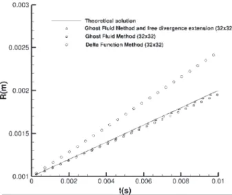
1000 kg m−3,Fig. 1. Comparison of the bubble radius temporal evolution between different numerical methods with a grid 32×32.
Table 1
Error on radius prediction with four different mesh size (32×32, 64×64, 128×128, 256×256) and for three different numerical methods.
32×32 64×64 128×128 256×256
Delta_function method −22.5% −23.7% −24.3% −24.6% Ghost fluid/simple velocity extension 2.2% 1.13% 0.611% 0.35% Ghost fluid/free divergence velocity extension 0.51% 0.22% 0.109% 0.056%
Table 2
Computational time (s) with the four different mesh size (32×32, 64×64, 128×128, 256×256) and for the three different numerical methods.
32×32 64×64 128×128 256×256
Delta_function method 1.29 13.3 166.5 3848
Ghost Fluid/simple velocity extension 1.52 15.3 198.9 4392 Ghost Fluid/free divergence velocity extension 1.63 18.0 246.1 5881
ρ
vap=
1 kg m−3,σ
=
0.07 N m−1,µ
liq=
0.001 kg m−1s−1,µ
vap=
1.78×
10−5kg m−1s−1. This test case does not require to solve the energy conservation equation, since the mass flow rate of phase change is imposed. A convergence study has been performed using three different methods to impose the velocity jump condition. The first one is the Delta Function Method where an interface thickness is introduced to smooth sharp discontinuities[29], the second one is the Ghost Fluid Method with a simple velocity extension[11,21], and the third one is the Ghost Fluid Method with a divergence-free ve-locity field extension[34]. For this test, the Delta Function Method requires to solve Eqs.(16)–(18), the Ghost Fluid Method requires to solve Eqs.(20)–(23)with the simple velocity field extension, and the further Eqs.(24),(25)must be solved to impose a divergence-free extension.A comparison between these three methods for the temporal evolution of the bubble radius has been plotted inFig. 1
for the coarsest grid. Other simulation results with finest grids are summarized inTable 1. The error on the bubble radius is computed thanks to the following relation:
ε
=
¯
¯
Rcomp(
tf)
−
Rtheo(
tf)
¯
¯/
Rtheo(
tf)
(34)We can notice that good results are obtained using Ghost Fluid Method with the simple velocity extension. However using the divergence-free extension slightly improves the accuracy. InTable 2, the computational costs of the different simulations are presented. As expected, the delta function method is faster than the Ghost Fluid Method, because some operations are duplicated when the latter is used. Moreover Table 2 also underlines the important additional cost resulting from the implementation of the divergence-free extension of the velocity field instead of simple velocity field extension. This can be easily explained by considering that a further Poisson equation must be solved at every time step when this extrapolation is used. We can extrapolate that for very refined grid this extension will involve twice as long computational time.
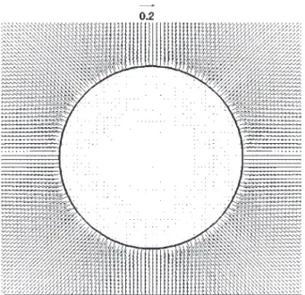
InFig. 2, the interface location and the vector velocity field have been plotted at the half time of the simulation with a grid (128
×
128) using the Ghost Fluid Method with a divergence-free velocity field extension. From this figure, the radial expansion flow around the bubble generated by the phase change be visualized.Fig. 2. Interface location and velocity field (m s−1) at time t=t
f/2 with a grid (128×128) using the Ghost Fluid Method with a divergence-free velocity
field extension.
At the opposite of Ghost Fluid Methods, the Delta Function Method provides poor predictions, since it converges towards a value higher of about 25% than the expected value (Table 1). This misleading behavior can be explained by the artifi-cial smoothing of the velocity field jump that can be observed in Figs. 3(a) and 5(a). We think this lack of convergence is not specific to the Level Set Method, but could also be observed with the Volume Of Fluid Method or the Front Track-ing Method, except if a specific velocity extrapolation or interpolation is developed to correct the error on the interface velocity.
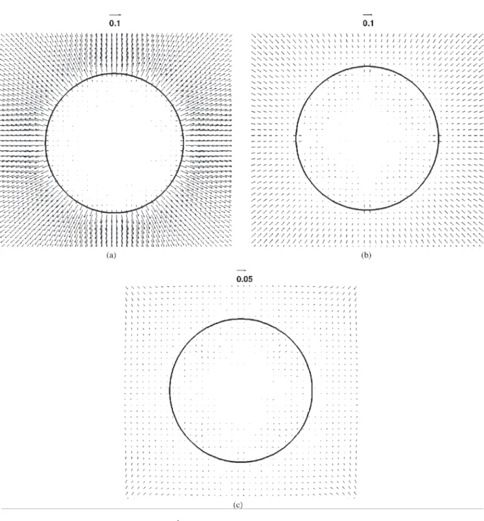
For example, this effect inherent to the smoothing of Dirac and Heaviside functions can be avoided by the use of ghost cells for the velocity as we can see onFigs. 3(b) and 3(c), where the vapor velocity fields and their extensions in the liquid domain are plotted. We point out that inFig. 3(b) the velocity field in the liquid phase points radially inwards the bubble. The constant extrapolation of the velocity field tends to zero at the interface, but not far from the interface. Indeed, the real velocity field tends to zero far from the interface, but a constant value of jump velocity is subtracted to this real velocity field in the whole domain. It results from this, the extrapolation of the velocity field which is presented in Fig. 3(b). Unlike the constant velocity field extrapolation, the divergence-free extrapolation leads to low values of the vapor velocity field extension everywhere in the liquid phaseFig. 3(c).
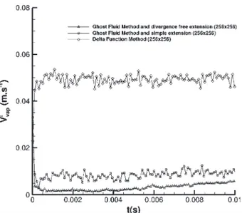
It is well-known that some spurious currents appear close to the interface when computations of a static bubble or droplet are performed with an interface capturing or an interface tracking numerical methods. These spurious currents are generated by grid effects when the curvature is computed to impose surface tension effects. When a phase change occurs, the intensity of spurious currents can strongly increase due to the jump condition on the velocity field. InFig. 4, the temporal evolution of the average of the vapor velocity magnitude at the interface has been plotted for the three different methods. This average of the vapor velocity magnitude is spurious because, in this test, the velocity field should be equal to zero everywhere in the vapor phase. This figure clearly highlights that the spurious currents at the interface are much stronger when the Delta Function Method is used, instead of the Ghost Fluid Method. It is noteworthy that the lack of convergence of the Delta Function Method, which has been previously reported in this section, can be explained by the important values of the velocity magnitude on the interface. Indeed inFig. 4, we can observe that, when the latter is used, these spurious currents are of the same order of magnitude as the interface velocity. It can also be deduced from this figure that the divergence-free extrapolation allows reducing substantially these spurious currents.
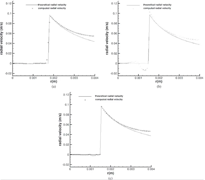
Finally, inFig. 5(a)–(c), the real radial velocity field component is plotted for the three methods at a given time. From
Fig. 5(a), it clearly appears that the zero level curve will be advected with an intermediate value of velocity between the vapor phase and the liquid phase, whereas with Ghost Fluid Method, the velocity field jump condition sharpness is perfectly maintained. Preserving the sharpness of the velocity field allows transporting interface with the appropriate velocity (vapor phase velocity, which is equal to zero for a static bubble) and not a mix at the interface between the velocities of the two phases.
To conclude on this simple preliminary test, we point out that for boiling flows, the phase change velocity has the same range as the radial expansion velocity. In a case where the radial expansion velocity is much faster than the phase change velocity (droplet vaporization), the numerical errors on the temporal evolution of the radius are much larger[34].
Fig. 3. (a) Interface location and fluid velocity field (m s−1) at t=t
f/2 with a grid (64×64) using the Delta Function Method. (b) Interface location, vapor
velocity field and its extension (m s−1) at t=t
f/2 with a grid (64×64) using the Ghost Fluid Method with a simple velocity field extension. (c) Interface
location, vapor velocity field and its extension (m s−1) at t=t
f/2 with a grid (64×64) using the Ghost Fluid Method and a divergence-free velocity
extension.
4.2. The Scriven test-case: growth of a static bubble in a superheated liquid
A more difficult test-case can be designed considering the growth of a static bubble in a superheated liquid. An analytical solution from[28]can be used to study the convergence of the different numerical methods, as it is proposed in[17,26]. This analytical solution is based on solving the following energy conservation equation in spherical coordinates:
∂
T∂
t+
ε
˙
R(
t)
R(
t)
2 r2∂
T∂
r=
α
µ ∂
2T∂
r2+
2 r∂
T∂
r
(35)where R(t
)
is the bubble radius depending on time,α
is the liquid diffusivity andε
=
1−
ρvapFig. 4. Temporal evolution of the spurious average velocity at the interface in the vapor phase in (m s−1) at time t
=tf with a grid (256×256) using the
three different methods.
We assume the following temporal dependence of bubble radius, where
β
is an unknown growth rate:R
(
t)
= β
√
α
t (36)Next by introducing the reduced variable s:
s
=
r2
√
α
t (37)we can derive the following integral solution for the temperature field:
T
(
s)
−
T∞ Tboiling−
T∞=
2β
3 Ja exp¡β
2+
2ε
β
2¢
+∞Z
s e(−x2−2εβ 3 x ) x2 dx (38)where Ja is the Jakob number defined as:
Ja
=
ρ
liqCpliq(
T∞−
Tsat)
ρ
vapLv(39)
with T∞ the liquid temperature far from the bubble (T∞
>
Tsat). Finally, considering the boundary conditions, an implicit equation is obtained for the growth rateβ:
Ja
=
2β
3exp¡β
2+
2ε
β
2¢
+∞Z
β e(−x2−2εβ 3 x ) x2 dx (40)Then, an iterative resolution of this implicit equation can be used to determine the corresponding value of
β
for a given value of the Jakob number. It is noteworthy that the theoretical solution depends on two dimensionless numbers (Ja andε
). We propose here a convergence study with Jakob number varying in a range of 3 to 10, and with a high density ratio between the vapor and the liquid (significant to the vapor water and the liquid water at ambient pressure conditions).All simulations are performed with the following physical properties,
ρ
liq=
958 kg m−3,ρ
vap=
0.59 kg m−3,σ
=
0.059 N m−1,µ
liq
=
2.82×
10−4kg m−1s−1,µ
vap=
1.23×
10−6 kg m−1s−1, kliq=
0.6 W m−1K−1, kvap=
0.026 W m−1K−1,Cpliq
=
4216 J kg−1K−1, Cpvap=
2034 J kg−1K−1, Lvap=
2.257×
106J kg−1, Tsat=
373 K.The simulations start at a time t0 with a bubble radius equal to 1 mm, until a time 4t0 required for the final bubble radius to be twice the initial radius (2 mm). The dimensions of the computational domain are lr
=
6 mm and lz=
12 mm. The initial conditions on the temperature field are determined using the analytical solution for the corresponding initial time. The simulations have been performed in a 2D axisymmetric configuration using the Ghost Fluid Method with a linear extension of temperature field and a simple velocity field extension (Table 3), a linear extension of temperature field and a divergence-free velocity field extension (Table 4), a quadratic extension of temperature field and a simple velocity field extension (Table 5) or a quadratic extension of temperature field and a divergence-free velocity field extension (Table 6). Due to the lack of consistence of results provided for the first case, the Delta Function Method has not been used on this moreFig. 5. (a) Comparison between the theory and the simulation on the radial velocity field at t=tf/2 with a grid (128×128) using the Delta
Func-tion Method. (b) Comparisons between the theory and the simulaFunc-tion on the radial velocity field at t=tf/2 with a grid (128×128) using the Ghost
Fluid Method. (c) Comparisons between the theory and the simulation on the radial velocity field at t=tf/2 with a grid (128×128) using the Ghost Fluid
Method and a divergence-free velocity extension.
Table 3
Error rate on the prediction of the bubble radius when varying the Jacob number for different computational grids using the Ghost Fluid Method with a linear extension for the temperature field and a simple velocity field extension.
Ja=3 Ja=4 Ja=5 Ja=6 Ja=7 Ja=8 Ja=9 Ja=10 64×128 21.2% 26.1% 30.2% 33.6% 36.3% 38.4% 40.1% 41.5% 128×256 9.3% 12.5% 15.7% 18.9% 21.9% 24.7% 27.3% 29.6% 256×512 0.8% 2.9% 5.3% 7.5% 9.3% 11.1% 13% 14.8%
difficult case. All the methods proposed have been tested with three different mesh size (64
×
128, 128×
256, 256×
512) and for 8 different values of the Jakob number.Tables 3–6highlight the convergence between the theory and the computations whatever the numerical method used. It also clearly appears that the accuracy decreases if the Jakob number increases. It can be explained considering that the thermal boundary layer thickness decreases if the Jakob number increases. From these tables, some important clarifications about the field extrapolation influence on the numerical accuracy can be provided. First of all, we observe that the quadratic extrapolation on the thermal field strongly improves the numerical predictions in comparison with the linear extrapolation. On the other hand, the divergence-free velocity field extrapolation does not provide an obvious improvement on the global
Table 4
Error rate on the prediction of the bubble radius when varying the Jacob number for different computational grids using the Ghost Fluid Method with a linear extension for the temperature field and a divergence-free velocity field extension.
Ja=3 Ja=4 Ja=5 Ja=6 Ja=7 Ja=8 Ja=9 Ja=10 64×128 20.1% 25.2% 29.5% 33.1% 35.7% 37.9% 39.6% 41.1% 128×256 8.5% 11.8% 15.1% 18.4% 21.4% 24.2% 26.8% 29.2% 256×512 0.01% 3.5% 5.8% 7.7% 9.5% 11.1% 12.9% 15.0%
Table 5
Error rate on the prediction of the bubble radius when varying the Jacob number for different computational grids using the Ghost Fluid Method with a quadratic extension for the temperature field and a simple velocity field extension.
Ja=3 Ja=4 Ja=5 Ja=6 Ja=7 Ja=8 Ja=9 Ja=10 64×128 9.5% 15.4% 5% 26.9% 31.3% 34.3% 37.7% 39.3% 128×256 0.002% 0.06% 1.25% 3.8% 7.2% 10.9% 14.7% 18.5% 256×512 4.0% 2.5% 2.5% 3.5% 3.5% 4.5% 3.5% 3.0%
Table 6
Error rate on the prediction of the bubble radius when varying the Jacob number for different computational grids using the Ghost Fluid Method with a quadratic extension for the temperature field and a divergence-free velocity field extension.
Ja=3 Ja=4 Ja=5 Ja=6 Ja=7 Ja=8 Ja=9 Ja=10 64×128 9.3% 15.0% 21% 26.2% 30.5% 33.8% 36.6% 38.7% 128×256 1.4% 1.6% 2.8% 5.0% 7.9% 11.5% 14.4% 17.6% 256×512 1.0% 0.4% 1.0% 1.0% 0.5% 0.5% 1.0% 2.0%
Fig. 6. Interface location and temperature field (◦C) for Ja=3 using the Ghost Fluid Method with a quadratic extension for the temperature field and a divergence-free velocity field extension with a grid (256×512) at initial and final time (a) t=t0, (b) t=4t0.
accuracy in comparison with the simple velocity field extrapolation. A gain in accuracy with the divergence-free velocity field extrapolation is only observed with the thinnest grid when the quadratic temperature extension is used. In this case, the agreement between theory and simulations is excellent whatever the Jakob number value. Determining a global order of accuracy is tricky, indeed the rate of reduction error strongly depends on the Jakob number and on the mesh resolution. For poorly resolved simulations with a high Jakob number, the convergence order is about one, but when the resolution increases, the error can be divided by 10 and sometimes more, which would correspond to order up to 3. These surprising results can be explained considering that the computation of the bubble growth rate computations strongly depends on the thermal boundary layer around the bubble. When the thermal boundary layer is poorly resolved with only 1 or 2 mesh points, determining a global accuracy order is not relevant.
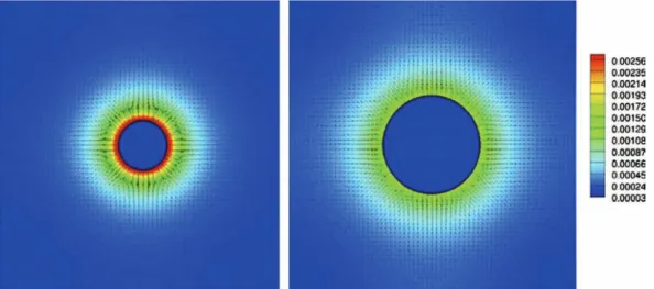
InFig. 6, the interface location and the temperature field have been plotted at the initial and at the final time for a Jakob number equal to 3, in order to visualize the thermal boundary layer thickness in regards to the bubble radius. FromFig. 7, we can see the radial expansion flow in the liquid around the bubble in this configuration.
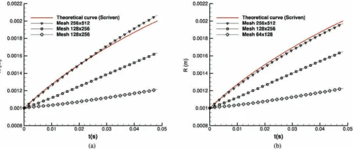
In Fig. 8, temporal evolutions of radius are plotted for three different mesh sizes and compared with the theoretical solution when the Jakob number is equal to 3.Fig. 8(a) corresponds to the computation with the quadratic extension for the temperature field and the simple velocity field extension, andFig. 8(b) corresponds to the computations with the quadratic extension for the temperature field and the divergence-free velocity field extension. It appears that the convergence rate is
Fig. 7. Interface location, velocity field and velocity magnitude (m s−1) for Ja=3 using the Ghost Fluid Method with a quadratic extension for the
tempera-ture field and a divergence-free velocity field extension with a grid (256×512) at initial and final time (a) t=t0, (b) t=4t0.
Fig. 8. (a) Convergence study for the temporal evolution of the computed radius at Ja=3 with the Ghost Fluid Method using a quadratic extension for the temperature field and a simple velocity field extension. (b) Convergence study for the temporal evolution of the computed radius at Ja=3 with the Ghost Fluid Method using a quadratic extension for the temperature field and a divergence-free velocity field extension.
not monotonic when a simple velocity field extension is used. Indeed, the numerical errors on the radius temporal evolution can be up or down the theoretical predictions. In such a case, the accuracy order of the method is more complicated to determine. On the other hand,Fig. 8(b) andTable 6show that the convergence rate is always monotonic if a divergence-free velocity field extrapolation is used.
This unusual behavior can be explained in all likelihood by considering that an underestimation of the temperature gradient at the interface leads to an underestimation of the phase change rate. From Eq.(20b), it leads to an overestimation of the vapor velocity field close to the interface. Thus, the two kinds of numerical errors have opposite effects on the global solution, leading to this unusual behavior where the sign of the global error can change when a grid convergence is performed. We can point out that the divergence-free extrapolation avoids this overestimation of the vapor velocity close to the interface, therefore this non-monotonic convergence is not observed when this extrapolation is used.
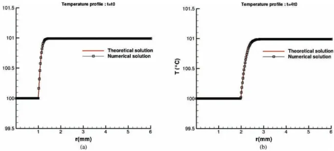
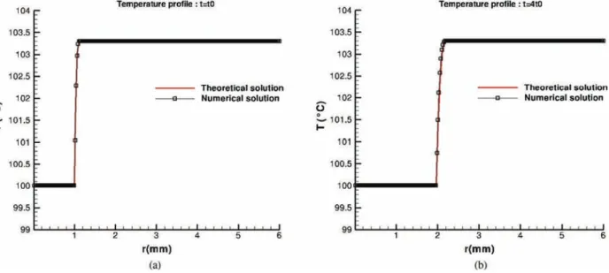
For this simulation, we have also plotted inFig. 9, the theoretical and the computed radial temperature profiles at initial and final time. At the first step, about 10 points are used to describe the thermal boundary layer around the bubble, it leads to very accurate predictions on the temporal evolution of the bubble radius.
High Jakob number simulations involve more drastic conditions with a thinner thermal boundary layer. InFig. 10, the temperature field and the interface location are plotted at the initial and the final time for a simulation with a Jakob number equal to 10. In this case, the thermal boundary layer is very thin in comparison to the bubble radius. The Radial expansion flow around bubble can also be visualized at the same times inFig. 11. InFig. 12, a comparison between the theoretical and
Fig. 9. (a) Initial condition on the radial temperature field for Ja=3 at t=t0, with a grid (256×512). (b) Comparison between the theory and the
computation of the radial temperature field for Ja=3 at t=4t0, with a grid (256×512) using a quadratic extension for the temperature field and a
divergence-free velocity field extension.
Fig. 10. Interface location and temperature field (◦C) for Ja=10 using the Ghost Fluid Method with a quadratic extension for the temperature field and a divergence-free velocity field extension for a grid (256×512) at initial and final time (a) t=t0, (b) t=4t0.
the computed radius temporal evolution is plotted for computations with a simple velocity field extension,Fig. 12(a), and divergence-free field extension,Fig. 12(b). In this case, the numerical simulations are well-resolved only when the thinnest grid is used. It can be easily explained considering that only 4 mesh points are used at the initial stage to describe the thermal boundary layer around the bubble, and about 8 points at the final stage of this simulation,Figs 13(a) and 13(b).
Finally, this test-case provides important results about the relevance of extrapolation techniques. It is shown that using a quadratic extrapolation, instead of a linear extrapolation, strongly improves numerical predictions. We also remark that a slight gain in accuracy is obtained when a divergence-free velocity field extrapolation is used instead of a simple velocity field extrapolation, but that gain is only remarkable when the thinnest grid is used.
4.3. The rising of a growing bubble
The last case deals with a growing bubble rising under the gravity effect (g
=
9.81 m s−2). Two different situations are considered; in the first one, the surface tension coefficient is high (σ
=
0.07 N m−1) and the bubble remains spherical at every time, in the second one the surface tension is low (σ
=
0.001 N m−1) and a deformation of the bubble occurs when the velocity increases. Initial radius R0is equal to 0.1 mm in the two cases, and the computational domain is lr=
1.2 mm,lz
=
2.4 mm. Unlike the computations of the previous section, the simulations start with a lower diameter in order to ensure that the Weber number is still minor than 0.1 for the simulation with a high surface tension coefficient, thus the bubbleFig. 11. Interface location, velocity field and velocity magnitude (m/s) for Ja=10 using the Ghost Fluid Method with a quadratic extension for the temper-ature field and a divergence-free velocity field extension for a grid (256×512) at initial and final time (a) t=t0, (b) t=4t0.
Fig. 12. (a) Convergence study for the temporal evolution of the computed radius at Ja=10 with the Ghost Fluid Method using a quadratic extension for the temperature field and a simple velocity field extension. (b) Convergence study for the temporal evolution of the computed radius at Ja=10 with the Ghost Fluid Method using a quadratic extension for the temperature field and a divergence-free velocity field extension.
remains spherical all along the simulation. Both computations are initialized using theoretical solution from[28] for the temperature field with a liquid superheat corresponding to a Jakob number equal to 3 at the time t0 corresponding to the initial bubble radius R0. The simulations are performed until the final time tf
=
16t0, in a moving frame at the average bubble velocity. We use the quadratic extension for temperature field and the divergence-free extrapolation for velocity field. The computational grid is 256×
512, which corresponds to the same ratio between the cell size and the initial bubble radius as for the static case with a grid 128×
256. Preliminary results (Fig. 8andTable 6) highlight that the cell size was good enough for static simulations with a Jakob number equal to 3. InFig. 14, the evolution of the temperature field and of the interface position can be visualized at four different times. As expected, the development of a thermal plume is observed at the rear of the bubble, whereas the thermal boundary layer at the top of the bubble is strongly flattened due to concurrent effects between the radial flow expansion and the rising motion.InFig. 15, we can visualize thanks to the streamlines of the flow, that the viscous boundary layer around the bubble is blown, by the radial flow at the interface. In[25], the authors developed a theory which predicts that the Nusselt number of the bubble increases linearly with the square root of the Peclet number, if the Peclet number is high:
Nu
=
4r
Pe
Fig. 13. (a) Initial condition on the radial temperature field for Ja=10 at t=t0with a grid (256×512). (b) Comparison between the theory and the
computation on the radial temperature field for Ja=10 at t=4t0, with a grid (256×512) using a quadratic extension for the temperature field and a
divergence-free velocity field extension.
Fig. 14. Interface location and temperature field (◦C) of a moving spherical bubble for Ja=3 using the Ghost Fluid Method with a quadratic extension for the temperature field and divergence-free velocity field extension for a grid (256×512) at different times (a) t=t0, (b) t=6t0, (c) t=11t0, (d) t=16t0.
Fig. 15. Interface location, streamlines flow and temperature field of a moving spherical bubble for Ja=3 using the Ghost Fluid Method with a quadratic extension for the temperature field and a divergence-free velocity field extension for a grid (256×512) at t=16t0.
Fig. 16. Nusselt number evolution vs square root of the Peclet number for a spherical bubble.
with the Peclet number defined as:
Pe
=
ρ
liqCpliqVbubbleD kliq(42)
with Vbubble the average bubble velocity, and D the diameter of the bubble. The Nusselt number is defined as the ratio between the thermal flux provided by the liquid to the rising bubble and a steady theoretical flux of heat conduction at the boundary of a static sphere (without any phase change):
Nu
=
qD kliq(
T∞−
Tsat)
=
ρ
vapLvap dD dt D kliq(
T∞−
Tsat)
(43)where q is the averaged surface density of the thermal flux at the boundary of the rising bubble. InFig. 16, a rather good agreement between this theoretical prediction and the direct numerical simulation is observed when the Peclet number is
Fig. 17. Interface location and temperature field of a moving non-spherical bubble for Ja=3 using the Ghost Fluid Method with a quadratic extension for the temperature field and a divergence-free velocity field extension for a grid (256×512) at different times (a) t=t0, (b) t=6t0, (c) t=11t0, (d) t=16t0.
high. InFigs. 17 and 18, the interface location and the temperature field evolution at different times can be visualized in the second case when the surface tension is low, which implies an important bubble deformation. The formation of a stagnation point at the top of the bubble is illustrated inFig. 19.
InFig. 20, a comparison of the Nusselt number evolution with the square root of the Peclet number is plotted both for the spherical bubble and for the deformed bubble. As expected, the Nusselt number is higher for the deformed bubble than for the spherical bubble when the Peclet number is fixed. That can be easily explained considering that the liquid–vapor surface exchange is higher for a deformed bubble than for a spherical bubble, considering the same Peclet number.
5. Conclusions
Direct numerical simulations of boiling flows have been performed using a Level Set/Ghost Fluid methodology. A first and simple test has been carried out, with a constant and uniform boiling flow rate. From that test, it has been shown that smoothing the velocity jump condition at the interface can lead to a misleading mass prediction, whereas the Ghost Fluid Method performs well that test. The use of extrapolation technique of discontinuous variables is an important feature of Ghost Fluid Method. Various extrapolation techniques have been described in literature [1,9,11,21,34], so one of the main objective of this paper was to study the influence of these extrapolations on the global numerical accuracy of the computation. It has been possible by using the theoretical solution of a static bubble growth in a superheated liquid. This extensive study points out that solving accurately the thermal boundary layer around the bubble and computing accurately the boiling mass flow rate are the “key-points” of the computation. Simulation results clearly show that these “key-points” are strongly improved when using a quadratic extrapolation on the temperature field instead of a linear extrapolation. An important result of this paper is the ability of the proposed numerical method to perform an accurate computation with a low resolution of the thermal boundary layer (less than 10 cells). This feature is of great importance, indeed usual situations can involve very thin boundary layer in comparison to bubble radius. Otherwise, the computational results are
Fig. 18. Interface location, streamlines of the flow and temperature field of a moving non-spherical bubble for Ja=3 using the Ghost Fluid Method with a quadratic extension for the temperature field and divergence-free velocity field extension for a grid (256×512) at t=16t0.
Fig. 19. Visualisation of the formation of a stagnation point using streamlines among the top of the bubble.
not very sensitive to the use of a divergence-free extrapolation, instead of a simple extrapolation, to extend the velocity field. It is an important difference with the results obtained in[34] for vaporizing droplets. Finally, computations of rising bubbles growing in a superheated liquid are performed successfully.
Some investigations on computational times of the different numerical methods have also been carried out, it appears that the divergence-free extension involves an important additional cost, especially for refined grids, which can lead to twice as long simulations. Unlike the divergence-free extrapolation on the velocity field, using the quadratic extrapolation, instead of the linear extrapolation, on the temperature field does not lead to a significant increase on the computational time
Acknowledgements
The authors gratefully acknowledge funding by CNES (Centre National des Etudes Spatiales) in the frame of the COMPERE program and by CNRS (Centre National de la Recherche Scientifique) for PhD Grant Support.
Fig. 20. Comparison between a spherical bubble and a non-spherical bubble of the Nusselt number evolution vs square root Peclet number. References
[1]T. Aslam, A partial differential equation approach to multidimensional extrapolation, J. Comput. Phys. 193 (2003) 349–355. [2]J.U. Brackbill, D.B. Kothe, C. Zemach, A continuum method for modeling surface tension, J. Comput. Phys. 100 (1992) 335–353.
[3]A. Esmaeeli, G. Tryggvason, A front tracking method for computations of boiling in complex geometries, Int. J. Multiph. Flow 30 (2004) 1037–1050. [4]A. Esmaeeli, G. Tryggvason, Computations of film boiling. Part I: Numerical method, Int. J. Heat Mass Transf. 47 (2004) 5451–5461.
[5]A. Esmaeeli, G. Tryggvason, Computations of film boiling. Part II: Multi-mode film boiling, Int. J. Heat Mass Transf. 47 (2004) 5463–5476.
[6]R. Fedkiw, T. Aslam, B. Merriman, S. Osher, A non-oscillatory Eulerian approach to interfaces in multimaterial flows (The Ghost Fluid Method), J. Com-put. Phys. 152 (1999) 457–492.
[7]Y. Ge, L.S. Fan, Three-dimensional simulation of impingement of a liquid droplet on a flat surface in the Leidenfrost regime, Phys. Fluids 17 (2005) 027104.
[8]Y. Ge, L.S. Fan, Three-dimensional direct numerical simulation for film-boiling contact of moving particle and liquid droplet, Phys. Fluids 18 (2006) 117104.
[9]F. Gibou, R. Fedkiw, L.T. Chieng, M. Kang, A second-order-accurate symmetric discretization of the Poisson equation on irregular domains, J. Comput. Phys. 176 (2002) 205–227.
[10]F. Gibou, R. Fedkiw, A fourth order accurate discretization for the Laplace and heat equations on arbitrary domains, with applications to the Stefan problem, J. Comput. Phys. 202 (2003) 577–601.
[11]F. Gibou, L. Chen, D. Nguyen, S. Banerjee, A level set based sharp interface method for the multiphase incompressible Navier–Stokes equations with phase change, J. Comput. Phys. 222 (2007) 536–555.
[12]M. Ishi, Thermo-Fluid Dynamic Theory of Two-Phase Flow, Eyrolles, Paris, 1975.
[13]D. Jamet, O. Lebaigue, N. Coutris, J.M. Delhaye, The second gradient method for the direct numerical simulation of liquid–vapor flows with phase change, J. Comput. Phys. 169 (2001) 624–651.
[14]G.S. Jiang, C.W. Shu, Efficient implementation of weighted essentially non-oscillatory schemes, J. Comput. Phys. 126 (1996) 202–228. [15]D. Juric, G. Tryggvason, Computations of boiling flows, Int. J. Multiph. Flow 24 (3) (1998) 387–410.
[16]M. Kang, R. Fedkiw, X.-D. Liu, A boundary condition capturing method for multiphase incompressible flow, J. Sci. Comput. 15 (2000) 323–360. [17]C. Kunkelmann, P. Stephan, Modification and extension of a standard volume-of-fluid solver for simulating boiling heat transfer, in: V European
Con-ference on Computational Fluid Dynamics, ECCOMAS CFD 2010, Lisbon, Portugal, 14–17 June, 2010.
[18]B. Lafaurie, C. Nardone, R. Scardovelli, S. Zaleski, G. Zanetti, Modelling merging and fragmentation in multiphase flows with SURFER, J. Comput. Phys. 113 (1994) 134–147.
[19]D. Legendre, J. Magnaudet, Thermal and dynamic evolution of a spherical bubble moving steadily in a superheated or subcooled liquid, Phys. Fluids 10 (6) (1998).
[20]X.-D. Liu, R. Fedkiw, M. Kang, A boundary condition capturing method for Poisson’s equation on irregular domains, J. Comput. Phys. 160 (2000) 151–178.
[21]D. Nguyen, R. Fedkiw, M. Kang, A boundary condition capturing method for incompressible flame discontinuities, J. Comput. Phys. 172 (2001) 71–98. [22]S. Osher, J.A. Sethian, Fronts propagating with curvature-dependent speed: algorithms based on Hamilton–Jacobi formulations, J. Comput. Phys. 79
(1988) 12–49.
[23]J. Papac, F. Gibou, C. Ratsch, Efficient symmetric discretization for the Poisson, heat and Stefan-type problems with Robin boundary conditions, J. Com-put. Phys. 229 (2010) 875–889.
[24]S. Popinet, S. Zaleski, A front-tracking algorithm for accurate representation of surface tension, Int. J. Numer. Methods Fluids 30 (6) (1999) 775–793. [25]E. Ruckenstein, E. James Davis, The effects of bubble translation on vapor bubble growth in a superheated liquid, Int. J. Heat Mass Transf. 14 (1971)
939–952.
[26]Y. Sato, B. Niceno, A sharp-interface phase change model for a mass-conservative interface tracking method, J. Comput. Phys. 249 (2013) 127–161. [27]R. Scardovelli, S. Zaleski, Direct numerical simulation of free-surface and interfacial flow, Annu. Rev. Fluid Mech. 31 (1999) 567–603.
[28]L.E. Scriven, On the dynamics of phase growth, Chem. Eng. Sci. 10 (1959) 1–13.
[29]G. Son, V.K. Dhir, Numerical simulation of film boiling near critical pressures with a level set method, J. Heat Transf. 120 (1998).
[30]G. Son, V.K. Dhir, Three-dimensional simulation of saturated film boiling on a horizontal cylinder, Int. J. Heat Mass Transf. 51 (2008) 1156–1167. [31]G. Son, V.K. Dhir, Numerical simulation of nucleate boiling on a horizontal surface at high heat fluxes, Int. J. Heat Mass Transf. 51 (2008) 2566–2582.
[32]M. Sussman, P. Smereka, S. Osher, A level set approach for computing solutions to incompressible two-phase flow, J. Comput. Phys. 114 (1994) 146–159. [33]M. Sussman, K.M. Smith, M.Y. Hussaini, M. Ohta, R. Zhi-Wei, A sharp interface method for incompressible two-phase flows, J. Comput. Phys. 221 (2007)
469–505.
[34]S. Tanguy, T. Menard, A. Berlemont, A level set method for vaporizing two-phase flows, J. Comput. Phys. 221 (2007) 837–853.
[35]G. Tomar, G. Biswas, A. Sharma, A. Agrawal, Numerical simulation of bubble growth in film boiling using a coupled level-set and volume-of-fluid method, Phys. Fluids 17 (2005) 112103.
[36]S.O. Unverdi, G. Tryggvason, A front-tracking method for viscous, incompressible multi-fluid flows, J. Comput. Phys. 100 (1992) 25–37. [37]S. Welch, J. Wilson, A volume of fluid based method for fluid flows with phase change, J. Comput. Phys. 160 (2000) 662–682.