O
pen
A
rchive
T
OULOUSE
A
rchive
O
uverte (
OATAO
)
OATAO is an open access repository that collects the work of Toulouse researchers and
makes it freely available over the web where possible.
This is an author-deposited version published in :
http://oatao.univ-toulouse.fr/
Eprints ID : 16891
The contribution was presented at ISBI 2016 :
http://biomedicalimaging.org/2016/
To cite this version :
Szasz, Teodora and Basarab, Adrian and Vaida,
Mircea-Florin and Kouamé, Denis Elastic-net based beamforming in medical ultrasound
imaging. (2016) In: 13th IEEE International Symposium on Biomedical
Imaging: From Nano to Macro (ISBI 2016), 13 April 2016 - 16 April 2016
(Prague, Czech Republic).
Any correspondence concerning this service should be sent to the repository
administrator:
staff-oatao@listes-diff.inp-toulouse.fr
ELASTIC-NET BASED BEAMFORMING IN MEDICAL ULTRASOUND IMAGING
Teodora Szasz
⋆Adrian Basarab
⋆Mircea-Florin Vaida
†Denis Kouam´e
⋆⋆
Universit´e de Toulouse, IRIT, UMR CNRS 5505, France
†Technical University of Cluj-Napoca, Romania
ABSTRACT
This paper presents a new way of addressing beamforming in ultrasound imaging, by formulating it, for each image depth, as an inverse problem solved using elastic-net regularization. This approach was evaluated on both simulated and in vivo data showing a gain in contrast, while maintaining an in-creased value of the signal-to-noise ratio compared to two standard ultrasound beamforming methods.
Index Terms— Ultrasound imaging, beamforming, in-verse problems, beamspace processing, elastic-net regulariza-tion
1. INTRODUCTION
Medical ultrasound (US) imaging (or sonography) is one of the most used imaging modalities due to its ease-of-use, low-cost, and non-ionizing characteristics.
Its principle is based on the interaction between the hu-man tissues and ultrasound waves produced by the US probe elements through their piezoelectric capabilities. Standard US probes are containing multiple elements (typically be-tween 16 and 256) that usually can form linear, annular, or circular arrays capable to both transmit the US waves to hu-man body and receive the reflected echoes by the tissues. These echos, transformed into digital signals, represent the raw data acquired by the ultrasound system.
Beamforming (BF) in reception offers the possibility to suppress the signals reflected by the sources in the scanned medium that are interfering with the desired ones. Thus, BF plays a key role in the improvement of the spatial resolution, the signal-to-noise ratio and the contrast of the beamformed image, also called radio-frequency (RF) image which is com-posed by multiple juxtacom-posed RF signals. For display pur-pose, some post-processing techniques like demodulation and log-compression are then applied to the RF signals in order to form the final US image, called B-mode (brightness mode im-age).
With the classical delay-and-sum (DAS) beamformer, the raw data is firstly focused to compensate the time-of-flight
de-This work has been supported by the CIMI Labex, Toulouse, France, under grant ANR-11-LABX-0040-CIMI within the program ANR-11-IDEX-0002-02.
lays, then weighted and summed up. The weighting is done through apodization functions (e.g. the Hanning window) in-dependent on the raw data. The quality in terms of resolution and contrast of DAS beamformer is limited. To improve the quality of the DAS beamformed images, a large variety of adaptive beamformers were proposed in literature, adapting the apodization coefficients to the raw data. The most used adaptive beamformer is minimum variance (MV) beamform-ers (e.g. [1]) which is inspired from the well known Capon filter. Based on the estimated covariance matrix, MV BF im-proves the contrast and the spatial resolution of the images, at the cost of increased computational time. Moreover, MV BF raises other problems, related to bad conditioned covariance matrices. Diagonal loading techniques (see e.g., [2]), time and spatial averaging [3], or the iterative adaptive approach (IAA) [4] can be used to overcome these limitations.
Instead of using fixed (DAS) or adaptive (MV) apodiza-tion funcapodiza-tions, we have recently proposed in [5] a new BF model for medical US imaging that takes into account the po-sitions of the elements and reflectors in order to relate the de-sired signals to the raw data. This results in an inverse prob-lem which use Laplacian or Gaussian priors through Basis Pursuit (BP), respectively Least Squares methods. We were thus able to obtain two complementary results, one that pro-duced sparse images and one generating smoother results [5]. This formulation also offered the possibility to highly reduce the number of US emissions during the scanning procedure, by integrating it with beamspace processing technique [6].
In this work we propose to further consider a compro-mise between sparsity and smoothness in the resulted images, by imposing an elastic-net regularization (see e.g. [7] and [8]). The proposed elastic-net (EN) beamformer minimizes a weighted sum of theℓ1 andℓ2-norms, with respect to the
data, therefore combining the advantages offered by the two norms.
2. BACKGROUND ON US BEAMFORMING Without loss of generality, we consider herein anM -element US probe, with the pitch (the spacing between elements) equal toλ2, whereλ = c
f0, withc denoting the speed of sound
in soft tissues, andf0 the transducer’s center frequency. A
angles,θk,k = 1, · · · K, and all the elements are used to
re-ceive the reflected echoes. After time-of-flight compensation, the raw data from allK directions have the size M × N × K, where N depends on the axial sampling frequency and the imaging depth.
In this configuration, the DAS BF process that generates one RF line for each steered emission can be expressed as:
ˆ
sk= wHyk, (1)
where yk ∈ CM×N is the time-compensated raw data
corre-sponding to thek-th emission, w is the apodization function of sizeM × 1, and (·)Hrepresents the conjugate transpose.
In contrast to DAS, MV BF adaptively calculates the apodization coefficients as:
wM Vk=
R−1k 1
1TR−1k 1, (2) where Rk = E[ykyHk] is the covariance matrix of ykand 1
is a lengthM column-vector of ones. These weights are then used to calculate the desired RF beamformed lines following (1).
3. PROPOSED ELASTIC-NET BASED BEAMFORMING
3.1. Direct model formulation
Contrarily to DAS and MV BF where the raw data is axially beamformed to form the RF signals, the proposed method is processing the raw data laterally, range by range. For a given rangen, n = 1, · · · , N , the direct model relating the desired signal to the data is given by:
ˆ
s[n] = (AHA)x[n] + g[n], (3) whereˆs[n] ∈ CK×1is a lateral scanline extracted from a
clas-sically beamformed image (e.g. DAS), A is a classical steer-ing matrix [9], x[n] is the desired signal and g[n] an additive white Gaussian noise. Note that for computational reasons, the model in (3) takes as input the classically beamformed data instead of the raw data (see e.g. [5] and [10]). To de-crease the number of US emissions required in BF process, the beamspace processing [11] technique can be applied to (3), thus decreasing the size of the data vectors[n] by a fac-ˆ tor ofK/P . After applying such a beamspace technique, the model in (3) can be written as:
z[n] = DHˆs[n] = (AHBSA)x[n] + D
Hg
[n], (4) where D of size K × P is the beamspace decimation ma-trix, AHBSof sizeP × M is the beamspaced steering matrix,
and x[n] of size K × 1 is the lateral profile at range n to be estimated. The model in (4) can be furthered considered as an inverse problem, where z[n] is the decimated DAS beam-formed data obtained forP < K emissions (the observations) and x[n] the desired lateral profile at depth n.
3.2. Model inversion
In this paper, we propose to solve the ill-posed inverse prob-lem in (4) using the following regularization referred to as elastic-net (EN) regularization:
xEN[n] = argmin x[n] (||z[n] − (ATBSA)x[n]||22 + γ(||x[n]||2 2+ ǫ||x[n]||1)), (5)
where|| · ||1and|| · ||22denote theℓ1, respectivelyℓ2-norms.
In our experiments, in order to decrease the number of hyper-parameters to tune, we consideredγǫ = (1 − γ), turning the regularization term in (5) into:
pen(x[n]) = γ||x[n]||22+ (1 − γ)||x[n]||1, (6)
wherepen(x[n]) is the penalization term that influences the sparsity of the result. Thus, forγ = 0 the problem turns into a basis pursuit algorithm, while whenγ = 1 we obtain the Tikhonov regularization. In the following, let us denote by Ψ∈ CP×Kthe measurement matrix formed as Ψ= AT
BSA.
Moreover, we define by Sγ the soft thresholding operator,
having the following function for anyγ > 0:
Sγ(t) = t −γ 2, if t< γ 2 0, if| t |≤γ2 t +γ2, if t<−γ2 (7)
Algorithm 1, based on [12], describes the main steps used to minimize the function in (5). We remind that this optimiza-tion is done independently, range by range, resulting into the consecutive lateral profiles of the final beamformed image.
Input:γ, z[n],Ψ Output: xp[n]
initialization: x0[n] = 0 // damping factor: τ = 2−γ1
// fix the step size using the matrix 2-norm of ΨΨT:
δ = normest(ΨΨ1 T
)×1.1
while convergence not reached do p := p + 1;
xp[n] =
τ SγKδ(xp−1[n] + δΨT(z[n] − Ψxp−1[n]);
end
Algorithm 1: Elastic-net beamforming of one lateral profile via Iterative Soft Thresholding.
4. RESULTS AND DISCUSSION
To evaluate the proposed method, we considered two cases: one that contains simulated data of 8 point reflectors arranged between 35 mm and 55 mm in depth and an experiment that
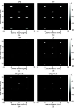
Fig. 1. (a) DAS, (b) MV, (c) BP, (d) LS, (e) EN (γ = 0.8), and (f) EN (γ = 0.2) BF results of a sparse medium.
uses in vivo data of a healthy thyroid. We compared our method with four other BF methods (DAS using Hanning apodization window, MV [2], BP and LS [5]) in the case of sparse medium, and with DAS, BP, and LS in the case of in vivodata.
4.1. Simulation results
The simulation containing the sparse medium was done us-ing the Field II program [13], aimus-ing to evaluate the BF lat-eral resolution of the proposed method. A 64-element US probe was used for both transmission and reception, with the center frequency, f0 = 4 MHz and 96% of relative
band-width. The transducer had the following element characteris-tics: the pitch of231 µm, the kerf of 38.5 µm, and the height of14 mm. An excitation pulse of two-cycle sinusoidal at f0
was used. K = 260 emissions were steered with angles be-tween−30 deg and 30 deg in the case of DAS and MV BF, and P = 260
5 = 52 emissions in the case of BP, LS, and
EN BF methods. The beamformed images are depicted in the Fig. 1. DAS BF (Fig. 1(a)) results in low lateral resolu-tion, further improved by MV BF (Fig. 1(b)). However, the best resolution of the target points is offered by the BP BF (Fig. 1(c)) that perfectly detects the 8 reflectors. This obser-vation is in coherence with the fact that BP privileges spar-sity in the results, through the Laplacian statistics. LS BF (Fig. 1(d)) results in smoother solutions compared with BP BF, but with better lateral resolution than MV. As expected, EN withγ = 0.8 (Fig. 1(e)) produces results similar with LS
4 2 0 2 4 6 8 25 20 15 10 5 0 8 Lateral distance [mm] Lateral profiles at depth of 45 mm
Amplitude [dB]
DAS MV LS EN ( =0.2)
Fig. 2. Lateral profiles of Fig. 1 at depth 45 mm.
DAS Lateral distance [mm] Axial distance [mm] 50 0 50 10 20 30 40 50 60 70 BP Lateral distance [mm] 50 0 50 60 50 40 30 20 10 0 LS Lateral distance [mm] Axial distance [mm] 50 0 50 10 20 30 40 50 60 70 EN ( =0.5) Lateral distance [mm] 50 0 50 60 50 40 30 20 10 0 (b) (d)
Fig. 3. (a) DAS, (b) BP, (c) LS, and (d) EN (γ = 0.8) BF results of in vivo data.
BF, since the hyperparameterγ decides the level of smooth-ness of the solutions, weighting the term related toℓ2-norm.
Contrarily, EN withγ = 0.2 (Fig. 1(e)) tends to the solution of BP BF. Note that for each simulation,γ has been set em-pirically to its best value.
The remarks above are confirmed by the Fig. 2 showing the lateral variation of the beamformed responses at depth45 mm. BP BF have the narrower mainlobes, offering the best delimitation of the points. However, the two cases of EN BF are presenting results that are varying between BP and LS, but with better spatial resolution of the target points than DAS and MV.
4.2. In vivo results
The data was acquired with the clinical Sonoline Elegra ultra-sound system, by using the 7.5L40 P/N 526028-L0850 linear array transducer of Siemens Medical Systems.
The beamformed images using in vivo thyroid data are presented in the Fig. 3. Three image quality metrics were considered, computed on the envelope-detected signals: the
Table 1. CR, CNR, and SNR values for the in vivo thyroid beamformed images in Fig. 3
BF Method CR[dB] CNR SNR DAS 12.4871 0.5546 0.2155 BP 20.4878 1.1304 0.3161 LS 16.9313 1.5643 0.6414 EN (γ = 0.5) 22.4489 1.4846 0.4571
contrast ratio (CR), the contrast-to-noise ratio (CNR), and the signal-to-noise ratio (SNR). Two regions,R1(the white circle
depicted in the Fig. 1(a)) andR2(the black circle depicted in
the Fig. 1(b)) were selected for calculating these metrics. CR is defined as [14]CR = |µR1 − µR2|, where µR1 andµR2
are the mean values in the regionR1, respectivelyR2. CNR is
defined as [15]CN R = |µR1−µR2| q σ2 R1+σ 2 R2
, whereσR1andσR2are
the standard deviations of intensities inR1, respectivelyR2.
The SNR was defined as the ratio between the mean valueµ and the standard deviationσ in the homogeneous region R2
[4]: SN R = µσ. The obtained values of CR, CNR, and SNR are depicted in the Table 1.
In Fig. 3(a), when using DAS BF the thyroid structure can be hardly distinguished, the contrast in the image being relatively low. Fig. 3(b) shows the result of the BP BF which selects the echoic structures of the image, thus eliminating most of the speckle in the image. Even if the CR and the CNR values are improved compared with DAS, the value of SNR is however comparable to DAS. As expected, LS results in more regular image at the price of lower contrast compared to BP, see Fig. 3(c). The best contrast of the beamformed image while maintaining a relatively high level of SNR and CNR is obtained with EN BF, see Fig. 3(d). In this case, the value of CR is increased by 10 dB compared with DAS, by about 2 dB compared with BP and by 5 dB compared with LS, see Table 1.
5. CONCLUSION
In this paper, we modeled US beamforming as an inverse problem regularized using elastic-net regularization. This for-mulation offers the possibility to integrate in the BF process the advantages of both sparse and smooth solutions. We have shown that our approach applied to simulated data provides solutions with improved lateral resolution compared to DAS and MV. Evaluated on in vivo data of a thyroid, the elastic-net based method improved the contrast of the image compared with DAS, BP, and LS methods. As a perspective we can con-sider generalized Gaussian priors that result inℓp-norm
min-imization together with taking into account the system point spread function.
6. REFERENCES
[1] J.-F. Synnevg, A. Austeng, and S. Holm, “Benefits of minimum-variance beamforming in medical ultrasound imaging,” IEEE
Trans-actions on Ultrasonics, Ferroelectrics, and Frequency Control, vol. 56, no. 9, pp. 1868–1879, Sept. 2009.
[2] B.M. Asl and A. Mahloojifar, “Minimum variance beamforming com-bined with adaptive coherence weighting applied to medical ultrasound imaging,” IEEE Transactions on Ultrasonics, Ferroelectrics, and
Fre-quency Control, vol. 56, no. 9, pp. 1923–1931, Sept. 2009.
[3] I.K. Holfort, F. Gran, and J.A. Jensen, “Broadband minimum variance beamforming for ultrasound imaging,” IEEE Transactions on
Ultrason-ics, FerroelectrUltrason-ics, and Frequency Control, vol. 56, no. 2, pp. 314–325, Feb. 2009.
[4] A.C. Jensen and A. Austeng, “The iterative adaptive approach in med-ical ultrasound imaging,” IEEE Transactions on Ultrasonics,
Ferro-electrics, and Frequency Control, vol. 61, no. 10, pp. 1688–1697, Oct. 2014.
[5] Teodora Szasz, Adrian Basarab, and Denis Kouam´e, “Beamforming through regularized inverse problems in ultrasound medical imaging,”
arXiv:1507.08184 [cs], July 2015, arXiv: 1507.08184.
[6] J.J. Fuchs, “Linear programming in spectral estimation. Application to array processing,” in , 1996 IEEE International Conference on
Acoustics, Speech, and Signal Processing, 1996. ICASSP-96. Confer-ence Proceedings, May 1996, vol. 6, pp. 3161–3164 vol. 6.
[7] Hui Zou and Trevor Hastie, “Regularization and variable selection via the elastic net,” Journal of the Royal Statistical Society: Series B
(Sta-tistical Methodology), vol. 67, no. 2, pp. 301–320, Apr. 2005. [8] Christine De Mol, Ernesto De Vito, and Lorenzo Rosasco, “Elastic-net
regularization in learning theory,” Journal of Complexity, vol. 25, no. 2, pp. 201–230, Apr. 2009.
[9] G.M. Kautz and M.D. Zoltowski, “Beamspace DOA estimation fea-turing multirate eigenvector processing,” IEEE Transactions on Signal
Processing, vol. 44, no. 7, pp. 1765–1778, July 1996.
[10] D. Malioutov, M. Cetin, and A.S. Willsky, “A sparse signal recon-struction perspective for source localization with sensor arrays,” IEEE
Transactions on Signal Processing, vol. 53, no. 8, pp. 3010–3022, Aug. 2005.
[11] Zhi Tian and H.L. Van Trees, “Beamspace MODE,” in Conference
Record of the Thirty-Fifth Asilomar Conference on Signals, Systems and Computers, 2001, Nov. 2001, vol. 2, pp. 926–930 vol.2. [12] Sofia Mosci, Lorenzo Rosasco, Matteo Santoro, Alessandro Verri, and
Silvia Villa, “Solving Structured Sparsity Regularization with Prox-imal Methods,” in Machine Learning and Knowledge Discovery in
Databases, Jos Luis Balczar, Francesco Bonchi, Aristides Gionis, and Michle Sebag, Eds., number 6322 in Lecture Notes in Computer Sci-ence, pp. 418–433. Springer Berlin Heidelberg, Sept. 2010, DOI: 10.1007/978-3-642-15883-4 27.
[13] J.A. Jensen and N.B. Svendsen, “Calculation of pressure fields from arbitrarily shaped, apodized, and excited ultrasound transducers,” IEEE
Transactions on Ultrasonics, Ferroelectrics, and Frequency Control, vol. 39, no. 2, pp. 262–267, Mar. 1992.
[14] Mengling Xu, Xin Yang, Mingyue Ding, and Ming Yuchi, “Spatio-temporally smoothed coherence factor for ultrasound imaging [Corre-spondence],” IEEE Transactions on Ultrasonics, Ferroelectrics, and
Frequency Control, vol. 61, no. 1, pp. 182–190, Jan. 2014.
[15] O.M.H. Rindal, J.P. Asen, S. Holm, and A. Austeng, “Understanding contrast improvements from capon beamforming,” in Ultrasonics