Deployment by a Shipper of a Collaborative Approach with its Carriers

(1)

© Guillermo Conte Moraga, 2019

Deployment by a Shipper of a Collaborative Approach

with its Carriers

Mémoire

Guillermo Conte Moraga

Maîtrise en génie mécanique - avec mémoire

Maître ès sciences (M. Sc.)

(2)

ii

Deployment by a shipper of a collaborative

approach with its carriers

Mémoire

Guillermo Conte Moraga

Sous la direction de :

Mikael Rönnqvist, directeur de recherche, Université Laval

Jean-François Audy, codirecteur de recherche, Université du Québec à Trois

Rivières

(3)

iii

Résumé

Un défi important dans l'industrie forestière consiste à réduire les coûts de transport globaux entre les fournisseurs et les clients. L'industrie forestière déplace de grandes quantités de bois des zones de récolte vers les terminaux et les usines. Lorsque de nombreuses organisations sont impliquées, une collaboration entre les fournisseurs et une utilisation efficiente des allocations permettent de trouver de meilleures solutions. Les allocations sont généralement basées sur des flux directs entre les nœuds d'approvisionnement et de demande. Cependant, de meilleures solutions peuvent être trouvées lorsque des itinéraires de retour en charge sont utilisés. Ceux-ci sont difficiles à trouver lorsque plusieurs parties prenantes sont impliquées, mais l'ajout d'informations provenant de la production de la récolte peut supporter une meilleure collaboration entre les fournisseurs ainsi que la détermination de plans plus efficients.

Le but de ce projet est d’élaborer un modèle capable de résoudre le problème de la livraison des multi-dépôts aux multi-clients, sur plusieurs périodes de temps, en minimisant les coûts de transport de différents types de bois. Proposer une nouvelle méthode pour le cas quand les clients seulement réceptionnent produits de fournisseurs fixés à l’avance. En outre, il analyse différentes méthodes de paiement des itinéraires de transport, afin de terminer un mécanisme qui incite les fournisseurs de transport à avoir recours au transport collaboratif. Nous décrivons les résultats obtenus avec une entreprise de pâtes et papiers au Québec, Canada.

(4)

iv

Abstract

One important challenge in the forestry industry is to reduce the overall transportation cost between suppliers and clients. The forestry industry moves large quantities of wood from harvest areas to terminals and mills. When many organizations are involved, a collaboration between the suppliers as well as an efficient use of allocations, achieve better solutions. Allocations are typically based on direct flows between supply and demand nodes. However, better solutions can be found when return trip routes are used. These are difficult to find when there are several stakeholders involved, but adding information from harvest production can establish better collaboration between suppliers as well as more efficient plans.

The purpose of this project is to define a model that can resolve the delivery from multi-depots to multi-customers, in a multi-period of time, minimizing the cost of transport for different types of timber. To propose a novel method for scenarios where the clients only receive products from pre-determined suppliers. Also, it analyzes different methods of transport payment for backhaul routes, in order to establish a mechanism that encourages the transport suppliers to use collaborative transport. We describe results obtained with a pulp and paper company in Quebec, Canada.

(5)

v

Table List

Table 1: Cost (dollars) of direct tours and backhauls between origin and destination. ... 12

Table 2: Demand and production per period and product. ... 12

Table 4: Details of transport cost. ... 14

Table 7: Summary of cost structures. ... 29

Table 8: Summary data of transactions of the first week in 2016. ... 30

Table 9: Conversion table between product units and DMT based on a full truck load. ... 31

Table 10: The shipper cost, operational cost of carriers and percentage of shipper cost reduction with direct tours as a basis of comparison. ... 35

Table 11: Shipper cost and movement by direct tours and backhauls with carrier collaboration. ... 36

Table 12: Operating time for all cost structures with time savings. ... 37

Table 13: Operational distances for all cost structures with distance savings... 38

Table 14: Summary of loading/unloading distances, time and fuel consumption for all cost structures. ... 39

Table 15: Fuel consumption for all cost structures with fuel savings. ... 40

Table 16: Average transportation cost for the 6 cost structures. ... 41

Table 17: Shipper cost and movements by direct tours and backhauls, when carriers work without collaboration. ... 54

(8)

viii

Figure List

Figure 1: An ilustration of direct tour. ... 7

Figure 2: An illustration of a backhaul route. ... 9

Figure 3: Log hauling truck travels on secondary road [18]. ... 10

Figure 4: General map with the positions of the facilities. ... 11

Figure 5: Original scenario of demand and production. ... 18

Figure 6: Modified scenario with the fictitious product C. ... 19

Figure 7: Direct tour system used in cost structure 1. ... 25

Figure 8: Backhaul route used in cost structure 2 ... 26

Figure 9: Backhaul route used in cost structure 3, with the restriction of 600 min. ... 27

Figure 10: Backhaul savings in cost structure 3A. ... 43

Figure 11: Backhaul savings in cost structure 3B. ... 43

Figure 12: Backhaul savings in cost structure 3C. ... 43

Figure 13: Backhaul savings in cost structure 4. ... 44

Figure 16: Backhaul savings in cost structure 3A. ... 46

Figure 17: Backhaul savings in cost structure 3B. ... 47

Figure 18: Backhaul savings in cost structure 3C. ... 47

Figure 22: Backhaul savings per week in cost structure 3A. ... 50

Figure 23: Backhaul savings per week in cost structure 3B. ... 51

Figure 24: Backhaul savings per week in cost structure 3C. ... 51

Figure 25: Backhaul savings per week in cost structure 4. ... 52

Figure 26: Backhaul savings per week in cost structure 5. ... 53

(9)

ix

Acknowledgments

I would like to thank Université Laval and FORAC for the opportunity of studying for my master’s degrees with a scholarship and finance support.

I would like to thank the partner that provided all the data for the analysis. I would like to thank my family for the support and encouragement they have shown all this time.

(10)

1

Introduction

General context

The forestry industry moves large quantities of wood annually, using for this purpose trucks, trains or a mix of both modes. The cost and time of transportation are important factors that need to be managed carefully. Some studies show that reducing empty truck trips by 11.6% can decrease transportation cost by 4%, which resulted in potential savings of more than $ 5,000,000 for a forest company in Canada [13].

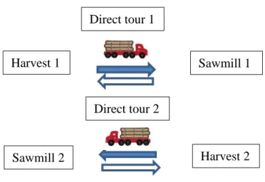
The forest transportation represents approximately one-third of the total cost in logistic planning [9], and for that reason several practices have been developed to manage and reduce the transportation costs. Time is a relevant variable, with a period of one year necessary to facilitate the tactical planning of forest transportation. The position of the harvest centers which feed the clients is an important point, but also their size and the system of movement with load utilized: direct tour or backhaul. Direct tour is a transport system that moves loads from origin to destination returning to the origin without a load and backhaul is a transport system that moves the load from origin to destination and from destination to origin.

Backhauls in forest transportation are an important logistics practice to reduce costs, because they improve the efficiency of the forest transportation system by achieving the transportation of a quantity of products in less time and distance than direct tour systems. While direct tours have only 50% of the transportation distance with truck loads, in backhauls this percentage is higher. Investigations such as Rönnqvist (2010) have noted that the range of savings in backhauls is typically between 2-10% [4], with reduction of overall transportation distance and reduction of fuel consumption.

In addition, the collaboration between carriers can improve the results, with a reduction of transportation cost. Carlsson et al. (2009) emphasize the importance of inter-company collaboration, for example in transportation planning, to improve companies’ results and reduce costs [1]. Karlsson et al. (2006) [6], developed a model where one of the aims was to understand which information and changes were necessary to create good coordination between contractors. Also, Palander and Vaatainen (2005) researched the benefit of

(11)

inter-2

company collaboration, presented a model with backhauls, where backhauls denoted a reduction of transportation cost by 2% in relation to cases without backhauls [2].

In previous forest transportation studies, authors developed an integer linear programing model of minimum cost for transporting different products daily to several clients using column generation; Rey, Munoz, Weintraub (2009) [16]; algorithm for reducing the time of empty transport at forestry industry, Gingras (2007) [13]; cost allocation methods in collaborative transportation based in cooperative game theory Guajardo and Rönnqvist (2015) [5] and Frisk, Göthe-Lundgren, Jörnsten, Rönnqvist (2010) [3]. Also, Frisk et al. (2016) [7], showed a model of transport that involve other aspects, such as production, inventory and idle time.

This master’s thesis will review the forest transportation of a Canadian pulp and paper company located in North America (hereinafter shipper). As part of its mission and values, in recent years it has been improving its production. Located in Quebec province, the mill has been improved with an investment of 2.5 billion dollars, achieving the best standard of safety and one of the best productions of fiber line pulp in North America.

The level of production of the shipper’s mill requires a big quantity of wood, which makes this mill the biggest consumer of wood harvested on private forest land in Québec province. Hence, the transportation of logs is one of the key variables that needs to be carefully managed by the shipper. Reducing the number of direct flows and transforming those routes into backhauls can improve the performance of transportation [12]. Forest transportation is an activity that represents a significant cost for a forestry company [9] and the shipper is no exception to the rule.

The shipper’s plans included a roadmap of 2015 with a strong focus on the competitiveness and sustainability of the business, meaning a goal that rests on eight priorities: safety, health, environment, quality, costs, productivity, trusted relationship and continuous improvement [10].

Improving the efficiency of actions, as well as of the actors, will allow the shipper to position itself as a world-leading reference in the sustainable management of the forestry industry. The importance of engaging every part of the business as much as possible will bring success to the company.

(12)

3

The model presented in this master’s thesis shows an alternative for minimizing the cost of transport of different types of product, from multi-depots to clients, in a multi-period delivery time. This model can program two time periods (or more) of product deliveries. To resolve this problem, the model is supported in some assumptions:

• The transport of the woods from the depot to the client is done in full truck loads [13].

• The trucks that end the tour in the same depot were the same one that started the trip.

• The model uses direct tours and backhauls for cover all the client’s necessities, because the trucks are full loading from depot to clients.

• There is no limit on the size of the truck fleet.

• The backhauls allow the transport of two different products (also one).

Also, this master’s thesis will review different forms of cost structures, the impact of the cost structures in the forestry transport and the system of transport with direct tour and backhauls. A novel method is developed when the clients receive products only from pre-determined suppliers designated by the shipper.

For this work, when a truck transports the product, the truck uses its full loading capacity. The capacity is measured in DMT (dry metric tons). The route time is based on the distance by type of road and average speed by type of road, but without consideration of the slopes of roads. Also, we are not considering speed reductions in protected zones or toll booths. Forest transportation research typically only considers log hauling trucks to cover the distances, without including other modes of transport such as train due to the short distances between clients and suppliers. This investigation covers a period of one year, working at the tactical planning level, being a useful tool for the operational planning.

The structure of this master’s thesis is the following: Chapter 1 shows the problem description and backhaul forest model. Chapter 2 shows the backhaul model with time periods and proposes an innovative approach to resolve scenarios where the clients receive

(13)

4

products from pre-determined suppliers. Chapter 3 describe the case study, reviewing the model and the objective function of every cost structure. Chapter 4 analyzes the results of the cost structures, and finally chapter 5 reviews the discussion of the research.

Objectives and contribution of the research

The first objective of the research is to measure the impact on a transportation plan that produces the cost of transport for both shipper and carriers, analyzing different forms of transport payment for backhaul routes that motivate the shipper and carriers to use backhaul.

The second objective and contribution is to develop a backhaul planning model with a restriction, where the clients receive products only from pre-determined suppliers, ensuring that the allocation of transportation satisfies the expectations of the shipper and carriers. That means reduction of transport costs and reduction of time-distance when the truck is without a load (empty).

(14)

5

1 Problem description

1.1 Transportation problem

The shipper starts with strategic planning over a long term (10 years). This time is necessary for the sustainable management of the resource, to achieve a viable production and reach a good size of trees for felling and delivery to the clients. After, the period of 10 years is divided in 2 periods of 5 years, for following up the growth of the species and the general state of the forest. With the information generated in strategic and tactical planning, the shipper proceeds with the annual harvest forest plan and finally the weekly planning with the carriers that transport the logs.

The tactical planning of transport between shipper, carriers and clients is very important for the procurement of every processing mill. According with that policy, the shipper and carrierswork with an annual schedule of production that could be adjusted once per month due to changes of demand. When the tactical planning is agreed, the next step is to fix transport of logs per week. This procedure is part of the operational planning and generate a support for next transport of logs.

In this case, the tactical planning tool used in the annual forest transportation problem is the backhaul model with periods. This linear programming model will allow to find the solutions of transport per week during a period of one year using backhauls.

1.2 Direct tours and backhauls forest model

The most common form of transport between supply nodes (origin) to demand nodes (destination) is through direct tours (Figure 1). This transport system moves loads from origin to destination returning to the origin without a load. This system achieves only a 50% of efficiency.

(15)

6 min 𝑍 = ∑ ∑ 𝐶_𝑖𝑗 ∙ 𝑋_𝑖𝑗 𝑛 𝑗=1 𝑚 𝑖=1 Subject to: ∑ 𝑋_𝑖𝑗 ≤ 𝑆_𝑖 𝑛 𝑗=1 , 𝑖 = 1, … , 𝑚 ∑ 𝑋_𝑖𝑗 ≥ 𝐷_𝑗 , 𝑗 = 1, … , 𝑛 𝑚 𝑖=1 𝑋_𝑖𝑗 ≥ 0, 𝑖 = 1, … , 𝑚; 𝑗 = 1, … , 𝑛

Here the variables are defined as:

𝑋𝑖𝑗 = 𝑓𝑙𝑜𝑤 (𝑙𝑜𝑔𝑠) 𝑓𝑟𝑜𝑚 𝑓𝑎𝑐𝑖𝑙𝑖𝑡𝑦 𝑖 𝑡𝑜 𝑐𝑢𝑠𝑡𝑜𝑚𝑒𝑟 𝑗, 𝑖 = 1, … , 𝑚; 𝑗 = 1, … , 𝑛

And the parameters are:

𝐶_𝑖𝑗 = 𝑢𝑛𝑖𝑡 𝑡𝑟𝑎𝑛𝑠𝑝𝑜𝑟𝑡𝑎𝑡𝑖𝑜𝑛 𝑐𝑜𝑠𝑡 𝑓𝑟𝑜𝑚 𝑓𝑎𝑐𝑖𝑙𝑖𝑡𝑦 𝑖 𝑡𝑜 𝑐𝑢𝑠𝑡𝑜𝑚𝑒𝑟 𝑗, 𝑖 = 1, … , 𝑚; 𝑗 = 1, … , 𝑛

𝑆𝑖 = 𝑠𝑢𝑝𝑝𝑙𝑦 𝑎𝑡 𝑓𝑎𝑐𝑖𝑙𝑖𝑡𝑦 𝑖, 𝑖 = 1, … , 𝑚 𝐷𝑗 = 𝑑𝑒𝑚𝑎𝑛𝑑 𝑎𝑡 𝑐𝑢𝑠𝑡𝑜𝑚𝑒𝑟 𝑗, 𝑗 = 1, … , 𝑛

This basic model has been very important for the development of the transportation problem. There are a lot of problems related with food, construction, trash transportation (only for mention some of them) that have been improved through this model.

(16)

7

Figure 1: An ilustration of direct tour.

The backhauls transport forest model is based in the previous research of Carlsson and Rönnqvist (2007) [12], as an alternative of solution for forest transportation. The model can solve big size of problems (big number of supply points and clients) in less time based in the procedure of column generation. This method, well-known as Column Generation, is used to solve LP models.

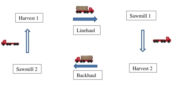
Figure 2 shows the backhaul transport system. While direct tours transport system uses a full truck loading only in one way, for transport the logs from harvests to clients, in backhauls one truck can cover all the demand of clients. The filled arrows with a truck show the routes where the truck is load with the product. In backhaul transport system is called linehaul the first way with truck load.

The following is the backhauls transport forest model:

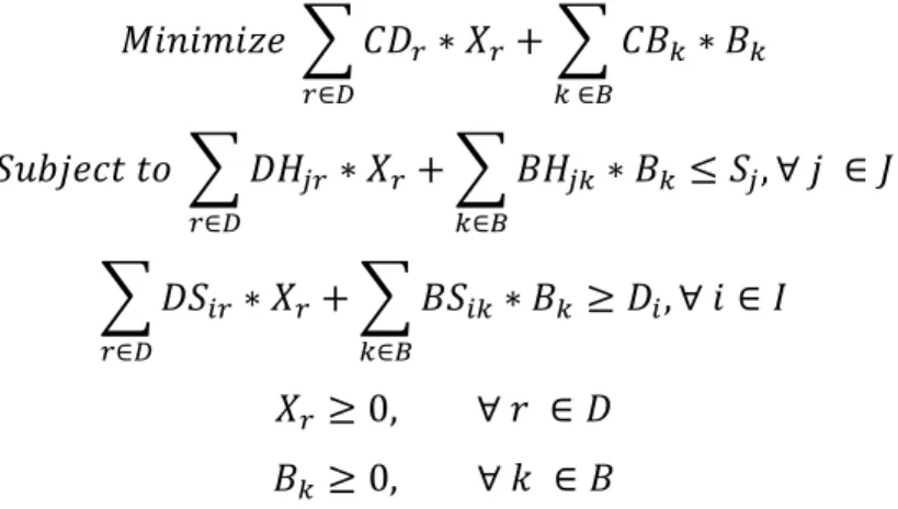
𝑀𝑖𝑛𝑖𝑚𝑖𝑧𝑒 ∑ 𝐶𝐷𝑟 𝑟∈𝐷 ∗ 𝑋𝑟+ ∑ 𝐶𝐵𝑘 𝑘 ∈𝐵 ∗ 𝐵𝑘 𝑆𝑢𝑏𝑗𝑒𝑐𝑡 𝑡𝑜 ∑ 𝐷𝐻_𝑗𝑟 𝑟∈𝐷 ∗ 𝑋_𝑟+ ∑ 𝐵𝐻_𝑗𝑘 𝑘∈𝐵 ∗ 𝐵_𝑘 ≤ 𝑆_𝑗, ∀ 𝑗 ∈ 𝐽 ∑ 𝐷𝑆_𝑖𝑟 𝑟∈𝐷 ∗ 𝑋_𝑟+ ∑ 𝐵𝑆_𝑖𝑘 𝑘∈𝐵 ∗ 𝐵_𝑘 ≥ 𝐷_𝑖, ∀ 𝑖 ∈ 𝐼 𝑋𝑟 ≥ 0, ∀ 𝑟 ∈ 𝐷 𝐵_𝑘 ≥ 0, ∀ 𝑘 ∈ 𝐵 Harvest Client

(17)

8

Where D is a set of direct tours, B is a set of backhauls, J is a set of harvest and I is a set of clients. Variables: 𝐵_𝑘 = 𝐹𝑙𝑜𝑤 𝑡𝑟𝑎𝑛𝑠𝑝𝑜𝑟𝑡𝑒𝑑 𝑖𝑛 𝑏𝑎𝑐𝑘ℎ𝑎𝑢𝑙 𝑘 𝑋𝑟 = 𝐹𝑙𝑜𝑤 𝑡𝑟𝑎𝑛𝑠𝑝𝑜𝑟𝑡𝑒𝑑 𝑖𝑛 𝑑𝑖𝑟𝑒𝑐𝑡 𝑡𝑜𝑢𝑟 𝑟 Parameters: 𝐶𝐷𝑟 = 𝐶𝑜𝑠𝑡 𝑖𝑛 𝑑𝑖𝑟𝑒𝑐𝑡 𝑡𝑜𝑢𝑟 𝑟 𝐶𝐵_𝑘= 𝐶𝑜𝑠𝑡 𝑖𝑛 𝑏𝑎𝑐𝑘ℎ𝑎𝑢𝑙 𝑘 𝐷_𝑖 = 𝐷𝑒𝑚𝑎𝑛𝑑 𝑐𝑙𝑖𝑒𝑛𝑡 𝑖 𝑆_𝑗 = 𝑆𝑢𝑝𝑝𝑙𝑦 ℎ𝑎𝑟𝑣𝑒𝑠𝑡 𝑗 𝐷𝐻_𝑗𝑟 = 1 𝑖𝑓 𝑑𝑖𝑟𝑒𝑐𝑡 𝑡𝑜𝑢𝑟 𝑟 𝑡𝑎𝑘𝑒𝑠 𝑝𝑟𝑜𝑑𝑢𝑐𝑡 𝑖𝑛 ℎ𝑎𝑟𝑣𝑒𝑠𝑡 𝑗, 0 𝑜𝑡ℎ𝑒𝑟𝑤𝑖𝑠𝑒 𝐵𝐻_𝑗𝑘 = 1 𝑖𝑓 𝑏𝑎𝑐𝑘ℎ𝑎𝑢𝑙 𝑘 𝑡𝑎𝑘𝑒𝑠 𝑝𝑟𝑜𝑑𝑢𝑐𝑡 𝑖𝑛 ℎ𝑎𝑟𝑣𝑒𝑠𝑡 𝑗, 0 𝑜𝑡ℎ𝑒𝑟𝑤𝑖𝑠𝑒 𝐷𝑆_𝑖𝑟 = 1 𝑖𝑓 𝑑𝑖𝑟𝑒𝑐𝑡 𝑡𝑜𝑢𝑟 𝑟 𝑑𝑒𝑙𝑖𝑣𝑒𝑟𝑦 𝑝𝑟𝑜𝑑𝑢𝑐𝑡 𝑖𝑛 𝑐𝑙𝑖𝑒𝑛𝑡 𝑖, 0 𝑜𝑡ℎ𝑒𝑟𝑤𝑖𝑠𝑒 𝐵𝑆𝑖𝑘 = 1 𝑖𝑓 𝑏𝑎𝑐𝑘ℎ𝑎𝑢𝑙 𝑘 𝑑𝑒𝑙𝑖𝑣𝑒𝑟𝑦 𝑝𝑟𝑜𝑑𝑢𝑐𝑡 𝑖𝑛 𝑐𝑙𝑖𝑒𝑛𝑡 𝑖, 0 𝑜𝑡ℎ𝑒𝑟𝑤𝑖𝑠𝑒

The objective function minimizes cost of transport in direct tours and backhauls. The first constraint ensures the quantity of products picked up from every harvest area is equal or less that the quantity generated. The second constraint ensures that the total quantity demanded for the clients of each product, is less or equal to the quantity that is transported from the harvest zones of the suppliers.

(18)

9

Figure 2: An illustration of a backhaul route.

1.3 Clients, suppliers and carriers

The clients (destination points) are mainly sawmills and pulp and paper companies that are located in the region of harvest zones. As part of the process of production, they need raw material that finally will be converted in: pulp, paper, kitchen furniture, etc.

The clients request different types of wood. That request depends on the product specifications of the clients.

The suppliers (origin points) are harvest zones where are harvested the logs. For transporting the logs, only one volume capacity of truck is considered on this research. The transport of the logs from origin to destination is done in consolidated loads. That means, using all the volume of the truck for transporting the products. The capacity can be measure in different units. The total number of trucks that are using in the transport is not relevant for this research.

Finally, the transaction of transport is measured in periods of one week. Every week has transactions that represent movements of trucks with products, between origin and destinations. Some weeks have more movements that others as well as other doesn’t have

Harvest 1 Client 1

Client 2 Harvest 2

linehaul

(19)

10

transactions. Weather conditions and some holidays are part of the reason for the absent of movement in some weeks.

1.4 Routes and routes cost

The routes are arcs that join nodes i with nodes j into the network. The nodes with index i are all the harvest zones, and the nodes j are all the clients.

There are primary roads and secondary roads. The primary roads are the highways and pavement routes. Classified as secondary routes, are all the forest roads, gravel or unpaved roads, as shows Figure 3.

The costs associated to the model have relation with the displacement between nodes and the time spent in every route. The cost is the same for one way to the other (symmetric). The cost of transport is in relation to diesel consumptions, time used and distance traveled.

Figure 3: Log hauling truck travels on secondary road [18].

1.5 Example

Two sawmills need to be fed with three different products on a weekly basis. In this scenario, there are three harvest locations that can provide the three types of wood which the clients need during 2 periods.

(20)

11 The products demanded by sawmills are:

• Product 1 • Product 2 • Product 3

The clients and suppliers are located at distances that are specified at the Figure 4. The costs of the transport are measure in time and distance. The system of transport is in direct tours and backhauls following the payment model used for the shipper. That means, for one direct tour is paid all the diesel consumption and time spent in transport and load-unload process; for linehauls is paid as direct tours and for backhauls is paid only the time spend in load routes. The cost of direct tours and backhauls are in Table 1.

Figure 4: General map with the positions of the facilities. Harvest Sawmill Harvest 2 Harvest 3 Harvest 1 Sawmill 2 Sawmill 1 200 km 220 km 100 km 15 km 20 km

(21)

12

Table 1: Cost (dollars) of direct tours and backhauls between origin and destination.

All the requirements of the two sawmills in all the periods must be fulfilled by the 3 harvest zones. The harvest zones have the same production as the demand per product of the clients per period. The detail of demand and production per period are in Table 2. All the quantities are in number of full trucks load. That means, for example, sawmill 1 needs for week1, 100 full trucks load of product 1.

Table 2: Demand and production per period and product.

The objective of the model is to minimize the cost of transport using a backhaul model. For this model, have been considered the following restrictions:

• All the requirements ordered by the clients must be fulfilled for the suppliers in all the periods.

• All the routes start and finish in the same depot.

Harvest Sawmill 1 Sawmill 2 Harvest Sawmill 1 Sawmill 2

1 290 310 1 260 250

2 30 160 2 25 130

3 150 25 3 120 20

Direct tour cost Backhaul cost

Demand Sawmill 1 Sawmill 2 Production Harvest 1 Harvest 2 Harvest 3

Product 1 100 0 Product 1 100 0 0

Product 2 200 150 Product 2 200 100 50

Demand Sawmill 1 Sawmill 2 Production Harvest 1 Harvest 2 Harvest 3

Product 3 200 400 Product 3 0 200 400

Week 1

(22)

13

• The loads are completed between suppliers and clients. The transhipment are not allowed.

The detail of the results is in Table 3. The table shows that are 6 types of direct tours and 4 types of backhauls for fulfilling the demand of clients.

Table 4 shows the details of how calculate the objective function the minimum cost of transport. For example, for transporting 1 full truck load from harvest 1 to sawmill 1, the direct cost is $290. If the total of full trucks in direct tours is 100, the total is $29,000.

In the case of backhauls for transporting 1 full truck from harvest 2 to sawmill 1 in line haul cost is $30 (the same of direct tours) and the cost of return in backhaul from harvest 1 to sawmill 2 is $250. As the total trucks in movement is 100, the total cost of backhaul is: $30 x 100 + $250 x 100 = $28,000. The total cost for the objective function is $ 256,250.

Direct tour Product Sawmill Harvest Week Quantity

1 1 1 1 1 100 2 2 1 1 1 50 3 3 2 1 1 300 4 1 1 3 2 100 5 2 1 3 2 300 6 3 2 3 2 100

Backhaul tour Product Sawmill Harvest Week Quantity

2 1 2 1 100 2 2 1 1 100 2 1 1 1 50 2 2 3 1 50 1 1 2 2 100 3 2 3 2 100 3 1 2 2 200 3 2 3 2 200 1 2 3 4

(23)

14

Table 4: Details of transport cost.

Harvest Sawmill Product Quantity Cost Direct Tour ($) Total ($)

1 1 1 100 290 29 000 1 1 2 50 290 14 500 1 2 3 300 310 93 000 3 1 1 100 150 15 000 3 1 2 300 150 45 000 3 2 3 100 25 2 500 199 000 Harvest Sawmill Product Quantity Cost Linehaul-Backhaul Tour Total

2 1 2 100 30 3 000 1 2 2 100 250 25 000 3 2 2 50 25 1 250 1 1 2 50 260 13 000 2 1 1 100 30 3 000 3 2 2 100 20 2 000 2 1 3 200 30 6 000 3 2 3 200 20 4 000

Total Cost Linehauls-Backhauls ($)(2) 45 250

Total Cost of Transport ($) (1+2) 244 250

(24)

15

2 Model and method

The backhaul model with periods allows planning the forest transport in tactical planning. With a vision over a year, the model permits a revision of tactical planning based in flow of products through backhauls [8].

The objective function of the model is minimizing the costs of forest transport. The first restriction ensures the quantity of products picked up from every harvest area is equal or less that the quantity generated by the period t of production. The second restriction ensures that the total quantity demanded for the clients of each product at each period, is the same quantity that is transported from the harvest zones of the suppliers.

Parameters 𝐷_{𝑖𝑝𝑡𝑣}ℎ = 1 𝑖𝑓 𝑑𝑖𝑟𝑒𝑐𝑡 𝑡𝑜𝑢𝑟 𝑣 𝑡𝑎𝑘𝑒𝑠 𝑝𝑟𝑜𝑑𝑢𝑐𝑡 𝑝 𝑎𝑡 𝑠𝑢𝑝𝑝𝑙𝑦 𝑖 𝑖𝑛 𝑡𝑖𝑚𝑒 𝑡, 0 𝑜𝑡ℎ𝑒𝑟𝑤𝑖𝑠𝑒 𝐵_{𝑖𝑝𝑡𝑘}ℎ = 1 𝑖𝑓 𝑏𝑎𝑐𝑘ℎ𝑎𝑢𝑙 𝑘 𝑡𝑎𝑘𝑒𝑠 𝑝𝑟𝑜𝑑𝑢𝑐𝑡 𝑝 𝑎𝑡 𝑠𝑢𝑝𝑝𝑙𝑦 𝑖 𝑖𝑛 𝑡𝑖𝑚𝑒 𝑡, 0 𝑜𝑡ℎ𝑒𝑟𝑤𝑖𝑠𝑒 𝐷_{𝑟𝑝𝑡𝑣}𝑠 = 1 𝑖𝑓 𝑑𝑖𝑟𝑒𝑐𝑡 𝑡𝑜𝑢𝑟 𝑣 𝑑𝑒𝑙𝑖𝑣𝑒𝑟𝑦 𝑝𝑟𝑜𝑑𝑢𝑐𝑡 𝑝 𝑡𝑜 𝑐𝑙𝑖𝑒𝑛𝑡 𝑟 𝑖𝑛 𝑡𝑖𝑚𝑒 𝑡, 0 𝑜𝑡ℎ𝑒𝑟𝑤𝑖𝑠𝑒 𝐵_{𝑟𝑝𝑡𝑘}𝑠 = 1 𝑖𝑓 𝑏𝑎𝑐𝑘ℎ𝑎𝑢𝑙 𝑘 𝑑𝑒𝑙𝑖𝑣𝑒𝑟𝑦 𝑝𝑟𝑜𝑑𝑢𝑐𝑡 𝑝 𝑡𝑜 𝑐𝑙𝑖𝑒𝑛𝑡 𝑟 𝑖𝑛 𝑡𝑖𝑚𝑒 𝑡, 0 𝑜𝑡ℎ𝑒𝑟𝑤𝑖𝑠𝑒 𝐶_𝑣𝑑 = 𝐶𝑜𝑠𝑡 𝑓𝑜𝑟 𝑑𝑖𝑟𝑒𝑐𝑡 𝑡𝑜𝑢𝑟 𝑣 𝐶_𝑘𝑏 = 𝐶𝑜𝑠𝑡 𝑓𝑜𝑟 𝑏𝑎𝑐𝑘ℎ𝑎𝑢𝑙 𝑘 𝐷𝑝𝑟𝑡= 𝐷𝑒𝑚𝑎𝑛𝑑 𝑜𝑓 𝑝𝑟𝑜𝑑𝑢𝑐𝑡 𝑝 𝑓𝑟𝑜𝑚 𝑐𝑙𝑖𝑒𝑛𝑡 𝑟 𝑖𝑛 𝑡𝑖𝑚𝑒 𝑡 𝑄𝑝𝑖𝑡 = 𝑃𝑟𝑜𝑑𝑢𝑐𝑡𝑖𝑜𝑛 𝑞𝑢𝑎𝑛𝑡𝑖𝑡𝑦 𝑜𝑓 𝑝𝑟𝑜𝑑𝑢𝑐𝑡 𝑝 𝑖𝑛 𝑠𝑢𝑝𝑝𝑙𝑦 𝑖 𝑖𝑛 𝑡𝑖𝑚𝑒 𝑡 𝑆 = 𝑆𝑢𝑝𝑝𝑙𝑦 𝐷 = 𝐷𝑒𝑚𝑎𝑛𝑑 𝑃 = 𝑃𝑟𝑜𝑑𝑢𝑐𝑡𝑠 𝑡𝑦𝑝𝑒𝑠 𝑇 = 𝑇𝑖𝑚𝑒 𝑝𝑒𝑟𝑖𝑜𝑑

(25)

16 Variables

𝑅_𝑣𝑡 = 𝑞𝑢𝑎𝑛𝑡𝑖𝑡𝑦 𝑜𝑓 𝑝𝑟𝑜𝑑𝑢𝑐𝑡 𝑑𝑒𝑙𝑖𝑣𝑒𝑟𝑦 𝑖𝑛 𝑑𝑖𝑟𝑒𝑐𝑡 𝑡𝑜𝑢𝑟 𝑣 𝑎𝑡 𝑡𝑖𝑚𝑒 𝑡 𝐵_𝑘𝑡 = 𝑞𝑢𝑎𝑛𝑡𝑖𝑡𝑦 𝑜𝑓 𝑝𝑟𝑜𝑑𝑢𝑐𝑡 𝑑𝑒𝑙𝑖𝑣𝑒𝑟𝑦 𝑖𝑛 𝑏𝑎𝑐𝑘ℎ𝑎𝑢𝑙 𝑘 𝑎𝑡 𝑡𝑖𝑚𝑒 𝑡

Multi-period Forest Transportation Model

𝑀𝑖𝑛𝑖𝑚𝑖𝑧𝑒 ∑ ∑ 𝐶𝑣𝑑 𝑣∈𝑉 ∗ 𝑅𝑣𝑡 𝑡∈𝑇 + ∑ ∑ 𝐶𝑘𝑏 𝑘 ∈𝐾 ∗ 𝐵𝑘𝑡 𝑡∈𝑇 𝑆𝑢𝑏𝑗𝑒𝑐𝑡 𝑡𝑜 ∑ 𝐷𝑖,𝑝,𝑡,𝑣ℎ 𝑣∈𝑉 ∗ 𝑅𝑣𝑡+ ∑ 𝐵𝑖,𝑝,𝑡,𝑘ℎ 𝑘∈𝐾 ∗ 𝐵𝑘𝑡≤ 𝑄𝑝𝑖𝑡, ∀𝑝 ∈ 𝑃, ∀𝑖 ∈ 𝑆, ∀𝑡 ∈ 𝑇 (1) ∑ 𝐷𝑟,𝑝,𝑡,𝑣𝑠 𝑣∈𝑉 ∗ 𝑅𝑣𝑡+ ∑ 𝐵𝑟,𝑝,𝑡,𝑘𝑠 𝑘∈𝐾 ∗ 𝐵𝑘𝑡≥ 𝐷𝑝𝑟𝑡 , ∀ 𝑝 ∈ 𝑃, ∀ 𝑟 ∈ 𝐷, ∀ 𝑡 ∈ 𝑇(2) 𝑅𝑣𝑡≥ 0, ∀ 𝑣 ∈ 𝑉 (3) 𝐵𝑘𝑡 ≥ 0, ∀ 𝑘 ∈ 𝐾 (4)

It is important to mention that in this model there is no flow connection between each time periods. It means is not used the inventory of one week to other.

Method to solve

The method used for solving the transportation problem, in practice the same model of one period, starts with the presentation of all possible direct flows between origin and destination. These are routes pre-designated by the shipper which connect harvest zones with

(26)

17

mills and product demanded. After, with all the direct tour shown, the model begins generating all possible backhauls. But this form of backhauls generation could take a long time, especially if there is a big quantity of harvest zones and mills as in this problem.

The method used for trying to find a solution to the problem with backhauls in a shorter computing time, consists in generating once all the possible alternatives. The method allows generating a pool of potential backhauls, avoiding generation of all backhauls and hence reducing the time to solve the problem. After the potential backhauls are generated, the objective function minimizes the cost of transportation and generates the optimal solution.

Method used when client receives products only from pre-determined suppliers

Until now, the method is considering all the combination routes that were possible for backhauls and direct tours, that means all suppliers that can meet clients’ requirements were used. But what happens when you must use specific suppliers designated by the shipper to fulfill the requirements of clients, even though there are best alternatives of supply to client allocation. In that case, the backhaul model with periods must choose the best alternatives with the restriction for using only one or some suppliers for certain clients. That restriction could be adapted to the model, but for that it is necessary to create new restrictions. In this research, to avoid implementing new restrictions, a novel approach is proposed, specifically new and fictitious products are created in order to respect the possible solution (i.e. shipper decision on supply to client allocation) where only suppliers and clients designated by the shipper can work together. Therefore, and going back to the novel approach proposed, if for example the shipper wants that the client 1 receives the same product A only from supplier 1 and 2 and leave the third supplier aside, with the implementation of a new fictitious product C, product A will be supplied only by supplier 1 and 2. The third supplier goes on with the production of product A, but all the product will be sold to client 2.

Figure 5 shows the original scenario of demand and production. The original scenario is the optimal solution of products flow between suppliers and clients without shipper decision on supply client allocation. The different colors of the lines to show the products flows between suppliers and clients: orange color represent the products flow from supplier

(27)

18

1 to client 1; blue color represent the products flow from supplier 2 to client 1 and client 2; green color represent the products flow from supplier 3 to client 1 and client 2.

Figure 6 shows the implementation form of fictitious product C. With the implementation of fictious product C, all the production of supplier 3 is going to client 2 and supplier 1 and supplier 2 sent all the production to client 1.

Figure 5: Original scenario of demand and production.

Supplier Client Supplier 3 Production :2A Supplier 2 Production : 2A Supplier 1 Production : 1A Client 1 Demand: 3A Client 2 Demand: 2A A A A A A Supplier 3 Production :2A Supplier 2 Production : 2C Supplier 1 Production : 1C

(28)

19

Figure 6: Modified scenario with the fictitious product C.

As fictitious product C is in fact product A, both clients receive the same quantity of Product A that they demand, but after the implementation client 1 only received from supplier 1 and 2.

Using the same example of section 2.5, where all requirements of two sawmills in all periods were fulfilled by 3 harvest zones, now the following restrictions, based on the shipper allocation decision will be used:

• Sawmill 1 receives product 3 only from harvest 3

• Sawmill 2 receives product 2 only from harvest 1 and harvest 2

Therefore, the requirements of sawmill 2 in relation to product 2 and the requirements of sawmill 1 in relation to product 3 will be open in two new fictitious products: product 4 and product 5. Product 4 will be the total product 2 sent by harvest 1 and harvest 2 to sawmill 2. Product 5 will be the total product 3 sent by harvest 3 to sawmill 1. The new fictitious products are created, because is necessary ensure that the shipper allocation decision is fulfilled, avoiding allocations with lower transport cost, but not designated by the shipper. The new production and demand are shown in Table 5:

Supplier Client Client 1 Demand: 3C Client 2 Demand: 2A 2A C 2C

(29)

20

Now, the new total cost for the objective function is $ 269,000; 4.98% more expensive than the results obtained in the example 1.5, where the shipper do not impose predeterminated allocation decision. The detail of the result appears in Table 6. The table shows that are 6 direct tours and 5 backhauls to fulfil the demand of clients.

Demand Sawmill 1 Sawmill 2 Production Harvest 1 Harvest 2 Harvest 3

Product 2 200 0 Product 2 200 100 50

Demand Sawmill 1 Sawmill 2 Production Harvest 1 Harvest 2 Harvest 3

Product 1 200 0 Product 1 0 100 100 Product 2 300 0 Product 2 0 0 300 Product 3 0 400 Product 3 0 200 400 Product 4 0 0 Product 4 0 0 0 Product 5 200 0 Product 5 0 0 400 Week 1 Week 2

(30)

21

Implementation

For computer results, the implementation of the forest transportation method was done with AMPL modeling system, solving the problem instances by CPLEX solver. The computer used is a 4 core i7 7th generation with 2.6 MHZ of processing speed.

The input data necessary to generate the optimal solution in the transportation process of this case is the following:

1. Distance: The distance between origin (supply) and destination (client) in kilometers. 2. Time: Time between origin and destination with the assumptions of average speed in

primary road, secondary road and on the road within 5 km distance from supply or client location.

3. Transactions every week, with the detail of origin, destination, product transported and carrier which made the transportation.

Direct tour Product Sawmill Harvest Week Quantity

1 2 1 1 1 50 2 3 2 1 1 200 3 1 1 3 2 100 4 2 1 3 2 300 5 3 2 3 2 300 6 5 1 3 2 200

Backhaul tour Product Sawmill Harvest Week Quantity

1 2 1 2 1 50 1 3 2 1 1 50 2 2 1 2 1 50 2 4 2 1 1 50 3 2 1 3 1 50 3 3 2 1 1 50 4 1 1 1 1 100 4 4 2 2 1 100 5 1 1 2 2 100 5 3 2 3 2 100

(31)

22

4. Cost of direct tours and backhauls in every route. 5. Name of: products, clients, carriers, harvest zones.

6. Contract between shipper and carriers, stipulating the payment formulas with the price of fuel and the ratio of payment per minute of transportation, and key assumptions as the time of loading/unloading per route, truck speed in primary and secondary road, truck speed on the road within 5 km distance from supply or client location and truck fuel consumption.

(32)

23

3 Case study

The case study of this research corresponds to a shipper, pulp and paper mill located in south of Quebec, Canada. The shipper manages a forest land located within a radius of 200 km from the mill. This investigation works with the historical forest transportation data provided by the shipper. Data include:

• Transportation zone: south of Québec, that span west to east over 160 kms., • Distances in primary and secondary routes between harvest zones and mills, • Time of transportation between origin and destination,

• Name of carriers and harvest zones,

• Truck speed assumptions and ratio of payments made by shipper to carriers.

In the case of products’ movement, the shipper provided a list of movements for 2016, with data of every transaction: quantity of product transported, client, harvest zone, carrier and date of transaction. Every client receives only one kind of product from an harvest zone that was pre-determined by shipper. Therefore, the origin, destination, product and route for every demand of logs were pre-determinated according to shipper decision, even though there are opportunities of less costly allocation.

3.1 Cost structures

The following subchapters review different transportation costs structured, as well as shipper payments to carriers. It is important to understand and measure the influence of every transportation cost on the objective function of transportation. Fuel, time, operation cost are part of the costs to be analyzed in this chapter. The cost structures that will review in detail are: cost structure 1, cost structure 2, cost structure 3A,3B,3C, cost structure 4, cost structure 5 and cost structure 6.

(33)

24

First, in cost structures 1, 2, 3A, 3B, 3C the analysis uses the shipper payment to understand what is the most convenient scenario for all the stakeholders. Also, to analyze how close every cost structure is to the minimum transportation time and minimum transportation distance.

Second, cost structure 4 measures the operation cost of carriers and how this cost is influenced by fuel and time costs. Also, cost structure 4 allows the analysis of decision behavior of carriers, and if such behavior is coherent with the shipper allocation.

Finally, cost structure 5 show the minimum transportation time and the cost structure 6 show which is the minimum transportation distance. This analysis allows checking what is the difference between operating times and distances with the optimal ones.

Cost structure 1

In cost structure 1, the objective function is minimizing the cost of transportation using only direct tours as a basic solution for forest transportation. Therefore, backhauls are not a part of solutions for transportation in this cost structure. Cost structure 1 is the basic solution of product flow and at the same time, the most expensive. In this case, payment is for all the fuel and time spent in round trips between origin and destination, including 90 minutes for loading/unloading. Payment for every minute spent is $1.34 dollars. In the case of fuel there is a surcharge tax of $0.288/liter, with a truck performance of 1.6 km/liter. Figure 7 shows the system of transportation used in cost structure 1.

The transport of products is from harvest to sawmill and at the return trucks are empty, achieving only a 50% of loading distance efficiency. The payment system pays the total time and operation distance, that means round trip between harvests and sawmill.

(34)

25

Figure 7: Direct tour system used in cost structure 1.

Cost structure 2 is the executed transportation scenario by the shipper in 2016. This cost structure uses direct tours and backhauls as a transportation system. The objective function is to minimize the cost of transportation using backhauls and direct tours. The shipper payment system pays for the fuel and time used as a round trip between origin and destination in all direct tours.

In a backhaul tour, the shipper pays two times the fuel and time spent between origin1 (harvest 1) and destination 1 (sawmill 1). The route between origin1 and destination 1 is designated as the linehaul. In addition, shipper pays the time spent between origin 2 and destination 2 (backhaul) and all the time of loading/unloading in the linehaul and the backhaul routes. The time for loading/unloading is fixed in 90 minutes, so that in a backhaul tour it is 180 minutes. Payment for every minute spent is $1.34 dollars. In the case of fuel, there is a surcharge tax of 0.288 $/liter, with a truck performance of 1.6 km/liter. Figure 8 shows the backhaul route used in cost structure 2.

Harvest 1 Sawmill 1

Sawmill 2 Harvest 2

Direct tour 2 2

(35)

26

Figure 8: Backhaul route used in cost structure 2

Cost structure 3A, 3B, and 3C

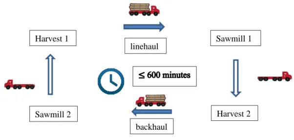
In cost structure 3A, 3B and 3C the same payment system of cost structure 2 is used but, a restriction of maximum time of tour is added. This restriction is of 600 minutes (10 hours) as a maximum time per tour. The limit of 600 minutes is fixed as a form of limiting the allowed work time limit for drivers per day. This time includes the loading/unloading time per route. The objective function is minimizing the cost of transportation, based on direct tours and backhauls. Figure 9 shows backhaul route used in cost structure 3A, 3B and 3C.

Cost structure 3A achieves the lowest cost among structures 3A, 3B, 3C, however, without restriction in unloading distance, the solution can include backhauls where overall empty truck distances are greater than overall loading distance. This cost structure is very attractive for shipper, but not for carriers, since some tours generate high operation cost for carriers, because of overall empty truck distances are bigger than overall full truck distances.

Harvest 1 Sawmill 1

Sawmill 2 Harvest 2

Linehaul

(36)

27

In the case of cost structure 3B a new restriction is added, the total unloading distance in backhaul must be less than 99% of the total loading distance in a route.

Finally, cost structure 3C increases the restriction on unloading truck routes by establishing that unloading routes cannot exceed 90 % of loading routes. This restriction improves the quality of the allowed backhaul, because reduce the distances where the truck is empty.

Figure 9: Backhaul route used in cost structure 3, with the restriction of 600 min.

In cost structure 4, the objective function is minimizing the operating cost of carriers. In this case the cost is per kilometers travel and the time spending by travel with or without a load, and the minutes spent in all trucks loading/unloading process. This cost structure gives us a good view of carrier costs, and how attractive the transportation opportunity is for them.

Operating costs of carriers include: - Driver salary, - Fuel liters. Harvest 1 Sawmill 1 Sawmill 2 Harvest 2 linehaul backhaul

(37)

28

The driver salary is composed for time of work and kilometers driving the truck. The ratio of payment is the following: $14.17 per hour of work and $ 0.17 per kilometer driven [15]. This salary is used for heavy truck drivers (road train) on Quebec regions . In the case of fuel, the carrier cost is $ 0.97 per liter, with an unloading truck performance of 1.8 km/liter and 1.6 km/liter when the truck is loading.

The objective function in cost structure 5 intends to minimize the operating time of transportation. The operating time includes the time to loading/unloading trucks and the time when the empty truck is travelling. This cost structure gives the best operating time to cover all the demand of clients during a year. Also, this cost structure is a good reference to compare with the total transportation time of other cost structures and measure the time gap. In this cost structure there are 2 type of costs, carrier operational cost and time shipper cost. The carrier operational cost includes the driver salary and fuel consumption cost and the shipper cost include only the time spent in allover forest transportation. The carrier operational cost pays the same ratios used in cost structure 4 and the shipper cost is $1.34/min.

Cost structure 6 intends to minimize the distance of transportation operation fulfilling clients’ demand over the year. With this cost structure it is possible to compare with others cost structures and measure the difference with the minimum distance of transportation operation. This comparison supports strong analysis to reduce fuel consumption, at a time of high diesel prices. This cost structure includes 2 types of cost, carrier operational cost and distance shipper cost. The carrier operational cost pays the same ratios used in cost structure 4 and 5. The distance shipper cost is fuel spent in the total distance travelled in the route with $0.97/liter and a truck performance of 1.6 km/liter.

(38)

29 Table 7 summarizes the six cost structures:

Table 7: Summary of cost structures.

3.2 Input data for case study

This information is used as a basis to simulate the transportation of all the cost structures during 52 weeks of the year, only changing the system of forest transport or the objective function according to the cost structure. Table 8 shows an example of summary data for the first week of transaction provided by the shipper. The information contains the following:

- Transaction: number of transactions. - Week: time period of transaction in 2016.

- Origin zone code: is the harvest zone of logs demanded by the client. - Destination client name: name of the client that demands the logs. - Demand: quantity of product demanded in dry metric tons.

- Carrier: name of the carrier that transports the products between origin and destination.

- Products: name of log species transported.

Cost Structure Operation time cost ($/min.) Fuel Cost ($/L) Labour Cost ($/hr.) Distance Cost ($/km.) Fuel Cost ($/L)

1 1.34 0.288 14.17 0.17 0.97

2 1.34 0.288 14.17 0.17 0.97

3A, 3B, 3C 1.34 0.288 14.17 0.17 0.97

Labour Cost ($/hr.) Distance Cost ($/km.) Fuel Cost ($/L)

4 14.17 0.17 0.97

5 14.17 0.17 0.97

6 14.17 0.17 0.97

Fuel Cost ($/L) 0.97 1.34

Shipper Cost Carrier Cost

Operation Time Cost

Distance Cost Operation time cost ($/min.)

(39)

30

Table 8: Summary data of transactions of the first week in 2016.

3.3 Clients, suppliers and carriers

This research considers 23 clients located in the province of Quebec. The clients are sawmills and pulp and paper companies. The harvest zones are 65 points of extraction of logs that are a part of shipper’s property. The service of 6 carriers is used for the products’ transportation, previously chosen by the shipper. The annual volume of product that moves each carrier during the studied year is the following:

- Carrier 1: 71,899 (dry metric tons) - Carrier 2: 40,546 (dry metric tons)

Transaction Week Origin Destination Demand (TMA) Products Carrier

1 w01 S38 C21 114.819 sciage feu Carrier 1

2 w01 S59 C13 456.03 pâte feu Carrier 1

3 w01 S37 C15 113.181 sciage res Carrier 2

5 w01 S38 C04 8.918 sciage cèdre Carrier 1

6 w01 S38 C14 20.442 déroulage feu Carrier 1

(40)

31 - Carrier 3: 5,372 (dry metric tons) - Carrier 4: 80,351 (dry metric tons) - Carrier 5: 9,582 (dry metric tons) - Carrier 6: 3,719 (dry metric tons).

3.4 Periods, trucks and products

This research considers 52 periods that represent the weeks of the year. Every week has transactions that are movements of trucks with products between origin and destination. Some weeks have more movements that others, and there are other without transactions. Whether and some holidays are part of the reason for the absence of movement in some weeks.

For products’ movements, only one volume capacity of truck is considered in this transportation process. This capacity is measured in DMT (dry metric tons). This capacity change depending on the transported product. Table 9 shows the values used by species of tree on the basis of a full truck load.

Table 9: Conversion table between product units and DMT based on a full truck load.

Unit Quantity (DMT)

Dry metric tonne 19

Green metric tonne 17.9

mlv 15.1

mlv - cedar 7.4

Green metric tonne 8.9

Thousand foot board measure-deciduous 18.4 Thousand foot board measure-cedar 13.9 Thousand foot board measure-resinous 19.1 cord 8 feet - resinous and cedar 13.5

(41)

32

The transportation of the logs from origin to destination is done in consolidated loads. That means using all the volume of the truck for transporting the products. The total trucks that are working in the transportation is not relevant for this research.

Regarding fuel consumption per truck, the operating cost of carriers considers 1.8 km/liter when the truck is empty, and 1.6 km/liter when the truck is loaded [17]. However, the agreement between shipper-carrier and the corresponding payment considers 1.6 km/liter as the truck consumption in both cases: loaded or empty.

Regarding the products, the clients request different types of product, depending on the companies’ necessities regarding the final product. The transportation process uses the pre-determinated allocation from the shipper, supplying different types of wood required by clients. This research uses the following products’ division, provided by the shipper:

- Deroulage Feuilleux - Pate Feuilleux - Sciage Cedre - Sciage Feuilleux - Sciage Resineux

This division is based on two big groups, Feuilleux and Resineux and subdivided into subgroups that represent the final use in the industry: sciage, pate and deroulage.

3.5 Routes and time restrictions

The routes are arcs that join nodes of index i with nodes of index j into the network. The nodes of index i are all the harvest places and the nodes of index j are all sawmills, or pulp and paper factories.

There are primary roads and secondary roads. Highways and paved routes are primary roads. All the forest roads, internal roads, gravel or unpaved road are classified as secondary routes. Approximately 30% of the distances between origin and destination were determined with the support of Google Maps. The other 70% is come from shipper data.

(42)

33

The average speed on primary roads is 75 km/h and on secondary roads is 25 km/h. Also, when the truck is 5 km from arriving to destination, the speed is 30 km/h. These are conditions of the truck speed that were accorded between shipper and carriers.

The cost of transportation in the model is related to the traveling and the time spent between the nodes. The cost is the same for one way or the other (symmetric). There are two cases of cost. First case is the ratio payment of shipper to carriers. The second case is the operating cost of carriers in relation to time and fuel. In the first case, shipper pays to carriers $ 0.288 per liter of fuel and $ 80.44 per hour of service. In the second case, operation cost of carriers, the price associated to diesel is the average between two regions: Estrie and Beauce [14]. For the purpose of this research, it is $ 0.97/liter.In the case of time and distance, cost is the salary of the driver with a ratio of $ 14.17 per hour of service and $ 0.17 per kilometer travel [15].

Regarding restrictions, one used in the model is the maximum time for every route. For this research, the maximum time per turn was fixed at 600 minutes, related to the maximum time designated that every driver can work per day. That means, the time per backhaul or direct tour can’t exceed that limit of time. This time includes the minutes used to load and unload the trucks (90 minutes per action). In the case of backhauls, it is 180 minutes and in the case of direct tour, 90 minutes.

Finally, the information for a week transaction is entered to the AMPL program and process to identify the result of every cost structure.

(43)

34

4 Results and data analysis

This chapter analyzes the results of every cost structure, describing the advantage of every cost structure, and what are the best values for operating cost, minimum distance, time and fuel consumption for products transported.

In the case study, the impact of backhauls is a reduction in unload distances of up to 8 % (104,840 km) and a reduction of spending times up to 2.25% (84,495 min.). When there is a collaboration between carriers, the impact of backhauls is stronger than in scenarios where carriers work alone.

From cost structure 1 to cost structure 3C are utilized direct tours and backhauls as systems of forest transportation. All these cost structures utilize the shipper payment form but, differ in the system of product transportation.

Cost structure 4 gives the minimum carrier operational cost, so this cost structure is a baseline of comparison for operating cost with cost structure 1 to 3C.

Cost structure 5 is the minimum operation time for all products transported that satisfied client’s demand. The minimum working time allows analyzing the behavior of time in all cost structures and which is the difference between the cost structure and the minimum time of product transportation.

Finally, cost structure 6 is the minimum traveling distance for transporting all the products from harvest zones to clients. This cost structure allows comparing the transportation distances of other cost structures with the minimum forest transportation distance.

4.1 Comparison of costs for all cost structures

The cost structures reviewed in this subsection support an analysis that clarify the cost of every cost structure, advantages/disadvantages, and the cost structure that improves the transportation costs of stakeholders.

(44)

35

The starting point of cost comparison of every cost structure is done with cost structure 1 as a basis (only direct tours). Cost structure 1 is the most expensive cost structure, with the highest cost for carriers and shipper, with longest distances for products movement.

Going on with other cost structures, it is important to mention that the shipper spent $ 5,625,980 dollars in forest transportation in 2016 (cost structure 2) for moving products from harvest zones to clients. The shipper used direct tours and backhauls as a system of transportation of logs. The shipper worked with 6 different companies of carriers.

Table 10 shows the shipper and carrier transportation cost for the different cost structures. Cost structure 1 is used as a basis for comparing. Also, in Table 10, the shipper cost showed in cost structure 6 include only fuel cost.

Table 10: The shipper cost, operational cost of carriers and percentage of shipper cost reduction with direct tours as a basis of comparison.

The results show that cost structure 2 is only 0.11% less than cost structure 1, where backhauls represent only 1% of overall DMT transported. That means that almost all the forest transportation used in 2016 was based on direct tours. Therefore, it is important to review the cost structure 3A, 3B and 3C, and understand what opportunities are being lost with the current form of operating.

Cost structure 3A reduced the shipper cost by 3.69% and carrier operating cost by 0.9%. This cost structure reduces the costs for both parts but, include some backhauls where empty distances are bigger than loaded distances. Such backhauls are not attractive for carriers, because they cover long distances without receiving a payment for that

Cost Structure Shipper cost Carrier operational cost Shipper cost reduction Carrier cost reduction

1 5 632 255 2 818 389 0.00% 0% 2 5 625 980 - 0.11% -3A 5 424 387 2 792 167 3.69% 0.90% 3B 5 471 479 2 738 068 2.96% 2.85% 3C 5 497 413 2 739 707 2.46% 2.79% 4 - 2 724 107 - 3.34% 5 4 927 052 2 724 128 2.01% 3.34% 6 1 512 668 2 724 115 0.54% 3.34%

(45)

36

displacement. Their costs are only 0.9% less than before, but their payment is reduced by 3.69%.

In the same line of cost structure 3A, cost structure 3B reduces the costs of shipper by 2.96% and decreases the operating cost of carriers by 2.85%. This cost structure is more attractive for carriers than 3A. First, cost structure 3B eliminates all backhauls that have more overall empty distance than overall loaded distance, and secondly, they reduce the operating costs. On the other hand, the shipper has a better cost structure than cost structure 1 and 2, but a little less attractive than cost structure 3A.

Revising cost structure 3C, the shipper cost appeared reduced by 2.46% in relation with cost structure 1, but 0.5% and 1.23% higher than cost structure 3B and 3A, respectively. The operating cost of carriers is 2.79% less than base case, but a little bit higher than cost structure 3B.

Reviewing the results of Table 11, backhauls represent only 1% of overall DMT transported in 2016. Also, cost structure 3A increment the percentage of backhauls representing 35% of the total tons transported. Cost structure 3A, 3B and 3C show that when is incremented the percentage of backhauls the cost of transport is reducing.

Table 11: Shipper cost and movement by direct tours and backhauls with carrier collaboration.

Regarding collaborative transportation, operating cost of carriers needs to be controlled so that working together has sense for carriers as well. Cost structure 4 shows the minimum operational cost for carriers, being a good point of comparison with other operating costs that are between cost structures 1 to 3C. As shown in Table 10, cost structure 4 offers

1 2 3A 3B 3C

Total shipper cost 5 632 255 $ 5 625 980 $ 5 424 387 $ 5 471 479 $ 5 497 413 $ Direct tour movement (DMT) 211469 209358 137852 163289 174359

Direct Tour/Total DMT transported 100% 99% 65% 77% 82%

Backhaul Movement (DMT) 0 2111 73617 48180 37110

Backhaul/Total DMT transported 0% 1% 35% 23% 18%

Total (DMT) 211469 211469 211469 211469 211469

Cost per ton. transported (Ton) 11.82 $ 11.81 $ 11.38 $ 11.48 $ 11.54 $ Cost Structure

(46)

37

an operating cost lower than other cost structures. The difference in percentage is the following:

- Cost structure 4 is 3.35% less than operating cost in cost structure 1 - Cost structure 4 is 2.43% less than operating cost in cost structure 3A - Cost structure 4 is 0.51% less than operating cost in cost structure 3B - Cost structure 4 is 0.57% less than operating cost in cost structure 3C

Therefore, cost structure 3B presents the most convenient operating cost for carriers, with 0.51% higher than cost structure 4.

Finally, when comparing carrier’s operating cost structure 5 (minimum time of transportation) and cost structure 6 (minimum distance of transportation) with cost structure 4, the difference between cost structures is $21 and $8 respectively (Table 10). Hence, when minimized the total transportation distance and total transportation time, the carrier operating cost is almost the minimum.

4.2 Comparison of time for all cost structures

Part of the goals searched by shipper, clients and carriers altogether is complete the total forest transportation in a minimum time. In the cost structures show in Table 12, cost structure 5 has the minimum time of forest transportation. The cost structure 3C is the minimum shipper cost between cost structures 1 to 3C. Also, Table 12 shows that cost structure 3B and 3C have almost 3 times more percentage of savings than cost structure 3A.

(47)

38

4.3 Comparison of distances for all cost structures

The minimum distance in all cost structures is cost structure 6, with 2,495,122 km. Between cost structures 1 to 3C, cost structure 3C offers the minimum total transportation distance with a 3.48% of reduction in distance compared to cost structure 1, as shown in Table 10.

Also, it is important to show that not necessarily a high quantity of backhauls implies the minimum cost of transportation. Going over the data in Table 13, cost structure 3A has more traveling distance in backhauls than other cost structures, but it only reduces the total distance of transportation by 1.12 %.

In addition, to analyze empty distances in backhauls for understanding the overall distance of full truck loading of each backhaul route. Table 14 shows that cost structure 3A has more empty distances than other cost structures, being less effective. Furthermore, cost structure 3C is less than 50 % of backhauls distance from cost structure 3A, but it reduces the total transportation distance by 3.48 %.

Table 13: Operational distances for all cost structures with distance savings.

Cost structure Direct tour Backhaul Total Savings Savings %

1 3761400 0 3761400 0 0.00% 2 3719890 - - - -3A 2412546 1325015 3737561 23839 0.63% 3B 2828908 860552 3689460 71940 1.91% 3C 3023482 665000 3688482 72918 1.94% 4 2861970 814941 3676911 84489 2.25% 5 2861712 815193 3676905 84495 2.25% 6 2874888 802147 3677035 84365 2.24%

(48)

39

Table 14: Summary of loading/unloading distances, time and fuel consumption for all cost structures.

4.4 Comparison of fuel surcharge for all cost structures

Cost structure 6 has the minimum total transportation distance and has the minimum consumption of fuel among all cost structures. Also, it is worth mentioning that cost structure

Cost Structure Direct Tour Backhaul Total Savings Savings %

1 2600024 0 2600024 0 0.00% 2 2568988 - - - -3A 1696336 874634 2570970 29054 1.12% 3B 1964496 546173 2510669 89355 3.44% 3C 2090256 419188 2509444 90580 3.48% 4 1991146 504006 2495152 104872 4.03% 5 1991006 504178 2495184 104840 4.03% 6 1999910 495212 2495122 104902 4.03% Distances Traveled (Km.)

Distance (Km) Time (Min) Unload distance (Km) Fuel consumption (L)

Direct tours 1696336 2412546 848168 1001309 Backhauls 874634 1325015 422790 517286 Total 2570970 3737561 1270958 1518595 Direct tours 1964496 2828908 982248 1159598 Backhauls 546173 860552 228409 325496 Total 2510669 3689460 1210657 1485095 Direct tours 2090256 3023482 1045128 1233832 Backhauls 419188 665000 164304 250583 Total 2509444 3688482 1209432 1484414 Direct tours 1991146 2861970 995573 1175329 Backhauls 504006 814941 199567 301145 Total 2495152 3676911 1195140 1476474 Direct tours 1991006 2861712 995503 1175247 Backhauls 504178 815193 199669 301245 Total 2495184 3676905 1195172 1476492 Direct tours 1999910 2874888 999955 1180502 Backhauls 495212 802147 195155 295955 Total 2495122 3677035 1195110 1476458 3A 3B 3C 4 5 6

Deployment by a Shipper of a Collaborative Approach with its Carriers

© Guillermo Conte Moraga, 2019

Deployment by a Shipper of a Collaborative Approach

with its Carriers

Mémoire

Guillermo Conte Moraga

Maîtrise en génie mécanique - avec mémoire

Maître ès sciences (M. Sc.)

Deployment by a shipper of a collaborative

approach with its carriers

Mémoire

Guillermo Conte Moraga

Sous la direction de :

Mikael Rönnqvist, directeur de recherche, Université Laval

Jean-François Audy, codirecteur de recherche, Université du Québec à Trois

Rivières

Résumé

Abstract

Table of Contents

Table List

Figure List

Acknowledgments

Introduction

General context

Objectives and contribution of the research

1

Problem description

1.1

Transportation problem

1.2

Direct tours and backhauls forest model

1.3

Clients, suppliers and carriers

1.4

Routes and routes cost

1.5

Example

2

Model and method

3

Case study

3.1

Cost structures

3.2

Input data for case study

3.3

Clients, suppliers and carriers

3.4

Periods, trucks and products

3.5

Routes and time restrictions

4

Results and data analysis

4.1

Comparison of costs for all cost structures

4.2

Comparison of time for all cost structures

4.3

Comparison of distances for all cost structures

4.4

Comparison of fuel surcharge for all cost structures