O
pen
A
rchive
T
OULOUSE
A
rchive
O
uverte (
OATAO
)
OATAO is an open access repository that collects the work of Toulouse researchers and makes it freely available over the web where possible.
This is an author-deposited version published in: http://oatao.univ-toulouse.fr/
Eprints ID: 16637
To cite this version: Belloc, Hervé and Chapin, Vincent and Manara, Francesco and Sgarbossa, Francesco and Meyer Forsting, Alexander Influence of the air inlet configuration on the performances of a paraglider open airfoil. (2016) International Journal of Aerodynamics, vol. 5 (n° 2). pp. 83-104. ISSN 1743-5447
Influence of the air inlet configuration on the performances
of a paraglider open airfoil
Hervé Belloc, Vincent Chapin, Francesco Manara, Francesco Sgarbossa and Alexander Meyer Forsting
Université de Toulouse ; Institut Supérieur de l'Aéronautique et de l'Espace (ISAE) ; 10 avenue Edouard Belin, 31400 Toulouse, France E-mail : [email protected] E-mail : [email protected] E-mail : [email protected] E-mail : [email protected] E-mail : [email protected]
Abstract: A finite volume flow solver was used to solve the Reynolds averaged
Navier-Stokes equations for the 2D flow field on a paraglider open airfoil. The canopy was assumed to be smooth, rigid and impermeable. The parametric study performed concerns the position and the width of the air inlet at the leading edge. The range of values used covers the air inlet geometries from classical ram-air parafoil to sport paraglider airfoil, including transition toward the full closed baseline airfoil. Results are focused both on lift and drag coefficients for performance analysis and on the internal pressure coefficient which can be critical for a real flexible wing regarding the risk of collapse. Depending on the appearance of a separation bubble over the upper edge, two well separated behaviours can be observed. The first behaviour is more typical of ram-air parachutes and the second one corresponds to the design of performance paragliders. For paraglider configurations, it is shown that the aerodynamic coefficients of the open airfoil can be easily deduced from the pressure coefficients of the baseline airfoil without solving the internal flow.
Keyword: air inlet, air inlet configuration, paragliders, paragliders airfoils, open
airfoils, ram air parafoils, ram air parachutes, separation bubble, pressure coefficients, internal pressure, aerodynamic coefficients.
Biographical notes:
Hervé Belloc is a graduate of the Conservatoire National des Arts et Métiers (C.N.A.M.) and currently a Research Engineer at ISAE in the “advanced aerodynamic and control” team. He was first aerodynamic tests engineer then wind tunnel manager. He is now in charge of aerodynamics and flight dynamics of gliding parachutes. His activity focuses on modelling, wind tunnel tests and flight tests. He work mainly for research projects about parachute guided air delivery system. Vincent Chapin is Professor of Aerodynamic at ISAE-SUPAERO. He develops research in the “advanced aerodynamic and control” team and is the specialist of aero-hydrodynamics of sailing. His research activity focus on innovative projects like fluidic control surfaces for Dassault-Aviation, twin-rig of the hydraplaneur for Y. Parlier, laminar keel design and wingsail for America's Cup and open-rotor aeroacoustic optimization for Airbus. He holds an engineer diploma from Polytech Orléans with a speciality in aerodynamics & structures, a master's degree in energy conversion and a PhD in unsteady numerical fluid mechanics from University Pierre & Marie Curie (Paris VI).
Francesco Manara received his Bachelor in Aerospace Engineering and his MS in Aeronautical Engineering from Politecnico di Milano, Dipartimento di Scienze e Tecnologie Aerospaziali in 2012 and 2015, respectively.
Francesco Sgarbossa received his Bachelor in Aerospace Engineering and his MS in Aeronautical Engineering from Politecnico di Milano, Dipartimento di Scienze e Tecnologie Aerospaziali in 2012 and 2015, respectively.
Alexander Meyer Forsting graduated with a MEng in Aeronautical Engineering from Imperial College London in 2014. He is currently working at DTU Wind Energy on his PhD thesis “Modeling wind turbine inflow”.
1 Introduction
Paraglider wings differ from rigid wings in several ways. To give the wing its structural integrity, a leading edge opening, which acts as a ram-air intake, is needed to maintain the canopy inflated. This opening is also called air inlet, or simply inlet, even though most of the time no flow enters when a steady state solution is considered. In fact it acts more as a pressure
inlet. In that way a paraglider airfoil is similar to a ram-air parafoil for gliding parachutes.
However, for performance purposes and without constrains like airdrop or parachute inflation, paraglider airfoils have the air inlet underneath the leading edge and further downstream. The inflated wing geometry remains stable only if the internal pressure remains greater than that of the external flow everywhere along the airfoil. A structural support can have a stabilizing effect in one way or another (e.g. arch strengthener or rigid ribs). As this form of support cannot easily be applied to the entire wing surface, this pressure condition remains a limitation for using such an airfoil at low angles of attack, which allow for higher flight velocities, and also for robustness in atmospheric turbulence.
Experimental investigations (Burk and Ware, 1967; Nicolaides et al., 1970; Ware and Hassell, 1969; Tribot et al., 1997), have established that the leading edge air inlet has a significant impact on the flow characteristics and thus the performance of a parafoil. These findings have been reproduced numerically by two- and three- dimensional potential flow computations performed by Ross (1993). He already pointed out that the limiting factor for the performance would be the structural integrity of the wing. To extend Ross’s approach to viscous flow phenomena, two-dimensional Reynolds-averaged Navier-Stokes (RANS) analyses were carried out by Mittal et al. (2001) and Balaji et al. (2005). They mainly focused on the developing instabilities due to the leading edge air inlet but also hinted at a smaller inlet improving the glide ratio. More recently
Mohammadi and Johari (2010) investigated the flow features which develop around the air inlet to explain these performance differences by using a refined structured mesh around the leading edge and a Spalart-Allmaras turbulence model replacing the Baldwin-Lomax model used previously. On a parafoil derived from the Clark-Y airfoil, he found a little reduction in the lift curve slope and a major effect on drag. He also suggests ΔCd = 0.5 h/c as a first estimate for the additional drag coefficient due to the air inlet, where c is the airfoil chord and h is the height of the cut.
Mashud and Umemura (2006) undertook wind tunnel experiments on an inflatable 3-D cell model. All preceding studies were concentrated on airfoils with cut off nose cones, creating a blunt body more characteristic for ram-air parachutes. Their study differs in such a way that it exhibits the transition from open to closed airfoil, once they started closing the air inlet by increasing the length of the upper lip. As they used flexible materials, the results included the effects of skin deformation. They noticed that the internal pressure varies with the squared sine of the angle between the air inlet and the free stream. They also showed that the internal pressure applied into the open airfoil modifies drag and lift at the air inlet region.
The airfoil studied in the present paper refers to an existing paraglider, with a chord length of 2.4 meters and which fly at a speed about 11 m/s. As a consequence, the free stream Reynolds Number in standard conditions is 1.8x10⁶. Consequently, airfoil geometry and Reynolds number are fixed but still realistic. The angle of attack varies from medium to relatively low values, representative of normal to accelerated flight, respectively. The main objectives are to quantify the influence of the position and the width of the air inlet on the aerodynamic performances and relate them to physical phenomena such as the appearance of separation bubbles. This is achieved by the analysis of the streamlines and pressure coefficient distributions. Results are
focused on lift and drag coefficients as well as internal pressure. The position value extends from forward air inlet, as it is for ram-air parachute airfoils, to an underneath and rear position as it is for paraglider airfoils. The width values extend from the closed baseline airfoil to one that is representative of sport paragliders. Thus, the transition from a parachute design to a paraglider design is covered, as well as the transition from the baseline closed airfoil to the paraglider open airfoil.
2 Numerical methodology
The 2-D simulation of the cross section of the airflow around a paraglider airfoil was obtained by solving the steady-state Reynolds Averaged Navier-Stokes equations (RANS) over a rectangular flow domain. The flow was considered incompressible with constant properties. For the free stream Reynolds Number of 1.8x10⁶, the turbulent Reynolds stresses were taken into account by choosing the turbulence model proposed by Spalart and Allmaras, (1992). Due to practical constraints, the interior of the paraglider was solved using the same turbulence model, regardless of the low Reynolds number in this area for which this model may not be well adapted.
The baseline closed airfoil and paraglider airfoil geometries were imported into the mesh generator software Gambit, which can build both structured, unstructured or hybrid meshes. Over the airfoils, a rectangular uniform structured mesh was used to analyse the boundary layer in the proximity of the canopy to its full extent. For the interior of the paraglider airfoil and the outer domain, an unstructured triangular mesh was used.
The mesh files were handled by the widespread finite volume flow solver FLUENT, which solves the RANS equations and manages the numerical simulations. The paraglider fabric was presumed rigid and impermeable. The boundary conditions on the computational domain
included uniform velocity at the inflow, upper and lower boundaries to allow for the freestream velocity V to enter at the specified angle of attack α (Figure 1). For the upper and lower boundaries, when the value chosen for the angle of attack results in an effective outflow, the solver automatically changes the condition to pressure outlet. The outflow condition was specified as pressure outlet. The no-slip boundary condition was applied to the interior and exterior surfaces of the airfoils. The numerical calculation was executed on a Linux workstation with one processor and two cores. The convergence of all numerical solutions presented is obtained with a second order numerical scheme.
In order to automate the mesh generation and the numerical simulation, the numerical framework VLab (V.Chapin et al.,2006), was used to define a specific parametrical script and run Gambit and FLUENT as a unique process. The main post-processing, which included the creation of streamlines, vorticity, internal and external pressure plots and other features, was also accomplished autonomously by this VLab script.
3 Mesh and domain sensitivity
There were no airfoil data sets available for the paraglider airfoil and its baseline closed airfoil. Nevertheless, a numerical simulation with the well-established software Xfoil (Drela 1989) was carried out for the baseline airfoil with a forced transition at 5% of the chord length.
As there was no experimental reference, and this study being closely related to the general approach of Mohammadi (2010), the same domain of 16x10 of the chord length was assumed to be valid. These dimensions refer to the domain extent in the chord direction and in the transverse direction respectively. The airfoil was placed halfway between the top and bottom boundaries, and five chord lengths from the inflow as shown in Figure 1.
The airfoil surface was covered by a boundary layer-type mesh and an unstructured triangular mesh elsewhere (Figure 2). In order to obtain a theoretical value of y+ of less than 2.5, necessary to ensure the existence of a grid point inside the viscous sublayer (Kalitzin et al.,2005), a first cell transverse dimension of 0.0055% of the chord length was employed. The Spalart-Allmaras model is one of the most sensitive to the location of the first cell center, therefore the condition for a maximal y+ value was analysed to ensure that the majority be below 5. For the baseline airfoil at α = 14°, it was found to be 5.60, nevertheless its value for α = 6° was more significant to the optimization and only 4.41. The leading edge inlet did not have a significant impact (max. 4.43), except in the very localized recirculationbubbles. There it reached up to 14 in the worst cases, but this was accepted as it was limited to very few cells.
In order to evaluate the mesh resolution effects, the rectangular-cell dimension on the airfoil surface and the height of the first rectangular cell above the surface were systematically modified. Moreover, the number of lines constituting the structured rectangular mesh refinement for the boundary layer and the growth rate of the unstructured triangular mesh were varied. Following each change in the mesh parameters, the resulting lift and drag coefficients were used as convergence criteria in regard to mesh sensitivity. Finally, the meshes around the baseline airfoil were composed of 78k cells and 69k nodes and the meshes around the paraglider airfoil were composed of 112k cells and 84k nodes.
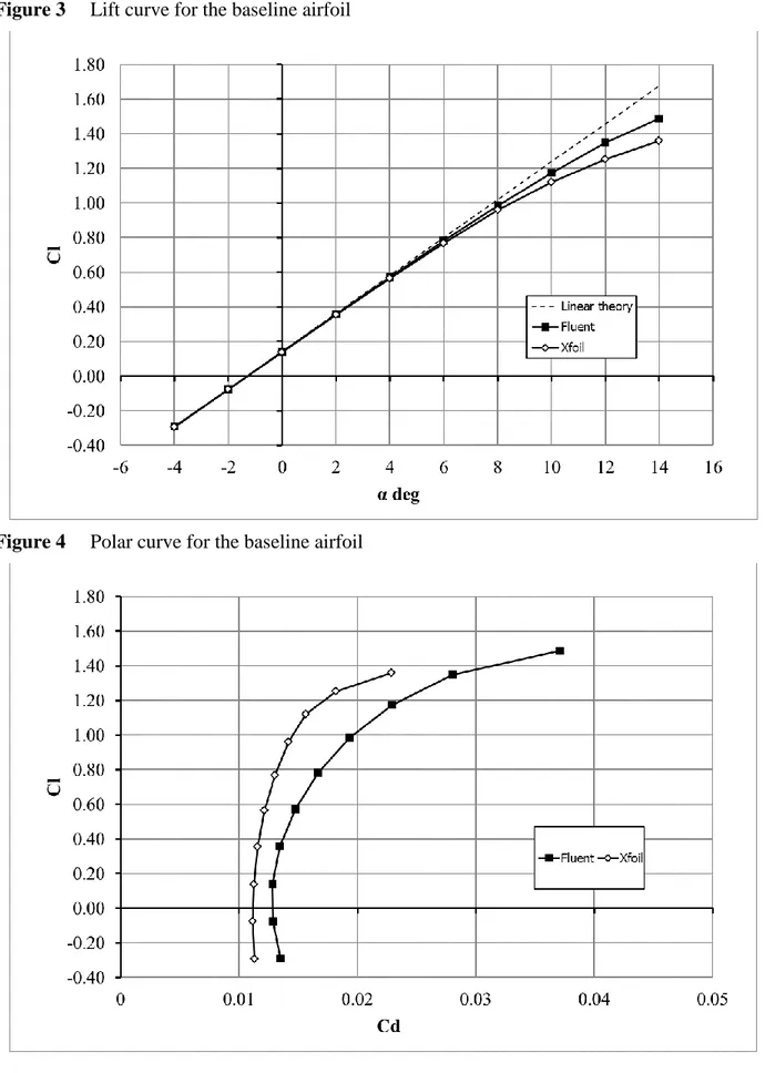
The resulting lift (Figure 3) and drag (Figure 4) curves were then compared to the results obtained using Xfoil for mesh validation. The computed lift coefficients did not exhibit significant differences in their linear part. However, the drag coefficients predicted by FLUENT were generally greater than the ones calculated by Xfoil. This behaviour can be explained by the
intrinsic tendency of FLUENT to overestimate the drag coefficient (Silva et al. 2002) and by the model’s assumption of a fully turbulent flow simulation.
In order to execute the automated computation, a mesh validation was performed using VLab with the same specifications (first row size etc.) for mesh generation. The mesh sensitivity analysis resulted in the following characteristics: 65 lines for the boundary layer refinement mesh (resulting in 0.098c for the total size of the structured rectangular mesh), 0.2c for the size of the wake zone and 15 mesh points on the edge of each boundary of the structured zone of the flow domain. A further refinement was implemented on the leading edge with a rectangular-cell dimension on the airfoil surface of 0.00125c chord length.
For the paraglider airfoil, an unstructured triangular mesh covered the interior computational domain. The interior mesh characteristics were adapted to the number of nodes of the leading edge refinement.
4 Results
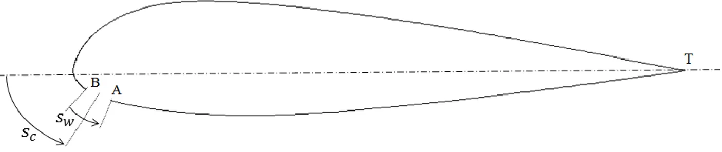
To respect the freestream Reynolds Number 1.8x10⁶ with a unitary chord at sea level, a freestream velocity of 26.4 m/s was selected. Three angles of attack, 2°, 4° and 6°, were investigated for each inlet configuration. For the most significant cases, the range was extended to -4° α 14° to exhibit the airfoil characteristics in more depth. For the paraglider airfoil, the air inlet parameters consisted of its width and of its position, with respect to its midpoint. The spline length of the width Sw, and the spline length between the leading edge and the midpoint of the inlet Sc, were normalized with the total spline length of the lower surface which is 1.027c (Figure 5), regardless of whether the air inlet extended over the upper surface which was sometimes the case. The following dimensions were analysed: Sw = [1% - 4%] in 1% intervals and Sc = [0%, 0.5%, 1%, 1.5%, 2%, 2.5%, 3%, 4%]. The parameters were chosen in this
particular way as this corresponds to the common limits used in paragliding and parachute production. The excessive position Sc = 5.3% was added. For each case, the lift and drag coefficients, as well as the vorticity contours, the streamlines and the pressure coefficient on all airfoil surfaces, were given as an output.
4.1 Baseline airfoil
The baseline airfoil had a thickness ratio of 18.5%. The lift coefficient Cl (Figure 3) displayed a linear dependence on the angle of attack α, for -4° α 8°, with a slope of 6.10 rad-1. This is slightly below the 6.28 rad-1 predicted by linear theory. The drag coefficient increases slightly from its minimal value 0.013, at α0, to 0.019 for α = 8°, and subsequently rises clearly. The
zero-lift angle of attack was found to be α0 = -1.3°, and the maximum glide ratio to be 51.2 at α = 10°.
Nevertheless, the analysis focused on α = 6°, as this is a more suitable angle of attack for a real 3D wing which receives additional induced and parasitic drag, due to the lines and the pilot. For α = 6°, the minimum pressure coefficient on the airfoil was Cp = -2.16, occurring on the upper surface between 0.09c and 0.095c (Figure 6). After this peak, the flow slows down, so that the pressure coefficient on the upper surface progressively recovers, and becomes slightly positive at the trailing edge. The stagnation point, Cp = 1, is situated on the lower side, right after the leading edge at 0.005c. Further downstream, the pressure on the lower surface decreases and stays close to zero, from 0.3c to the trailing edge. Since the pressure on the lower surface is always greater than the pressure on the upper surface, lift is generated all along the airfoil. At this angle of attack there is no flow separation, and the vorticity contours (Figure 7) display a fully attached boundary layer, which thickens along the two surfaces toward the trailing edge. The boundary layer on the suction side nearly doubles compared to the boundary layer on the pressure side.
4.2 Flow analysis around the leading edge
This section presents a physical description of various flow patterns obtained in the region of the leading edge. Before this, a more general remark must be made on the internal flow. At the interior of the paraglider airfoil, some vortices of considerable dimensions are displayed. Their number and extent either depends on the configuration of the air inlet or the angle of attack. For instance, Figure 8 shows, for the case α = 8° with Sc = 2%, Sw = 1%, which is detailed later, the values of the turbulent viscosity ratio inside and around the airfoil. The internal value reaches 60 in the core of these vortices. On the external side, the value is about 170 in the boundary layer and 350 in the wake. However, the turbulence model adopted is not optimal for these low Reynolds number phenomena, and no wind tunnel experiments are available to observe and validate this output. In addition, the interior velocity is almost zero everywhere, so the streamlines showing these vortices are somewhat misleading in this practically stagnation area. As a matter of fact, the internal pressure has a constant value, except for a restricted area near the air inlet.
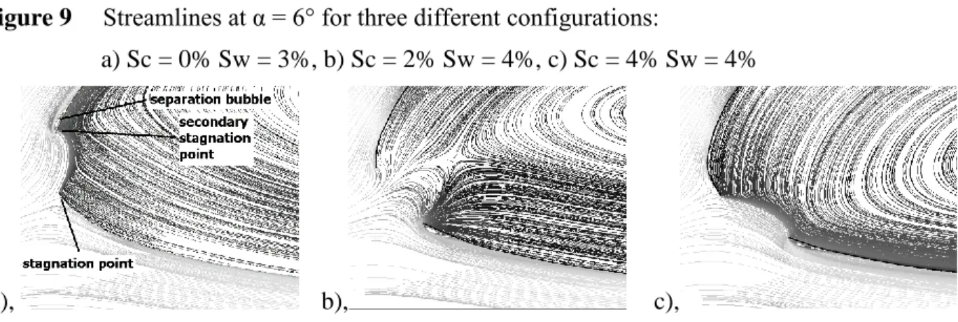
Referring to the main stream direction, the stagnation point can precede, coincide with, or follow the air inlet, depending on the position of the inlet and on the angle of attack. When the stagnation point is located after the air inlet on the lower surface (Figure 9a), the flow along this surface is nearly unperturbed by the presence of the air inlet itself. This situation happens with an air inlet oriented ahead and/or an increased angle of attack. To the contrary, the flow along the upper surface is disturbed and the boundary layer is thicker than that of the baseline airfoil. This effect is more obvious when the air inlet width is increases. Moreover, especially if the width rises, a larger amount of air can penetrate the airfoil. Subsequently, it has to circumvent the solid canopy to exit, thus resulting in an additional stagnation point at the interior of the leading edge.
A strong separation bubble appears on the external surface, at the front end. Circulation and boundary layer are altered, decreasing the lift coefficient and increasing the drag coefficient.
When the stagnation point is just before the air inlet in the leading edge area (Figure 9c), the physical behaviour is a mirror image of the one illustrated above. A second stagnation point appears at the opposite inlet end, or at the interior of this end, toward the lower surface. A separation bubble can form on the external surface of the inlet end. In this case, the lift coefficient is not decreased but a negative effect on the drag coefficient is still present. As for the previously analysed case, when a separation bubble occurs the boundary layer is thicker than for the baseline airfoil. Here the phenomenon is less significant. When the beginning of the air inlet is further downstream, its distance to the stagnation point increases. As a consequence, when the flow reaches the air inlet, it has had a larger distance to accelerate and has become tangent to the canopy (Figure 10). Hence, the deflection of the fluid, which penetrates the canopy, is reduced. However, the internal pressure decreases, this will be examined in more depth in the following section.
When the stagnation point coincides with the air inlet as in Figure 9b, it is located inside the airfoil and stays behind the upper or the lower leading edges. For increasing values of the air inlet width, external separation bubbles can form on one or both of the air inlet ends. On the other hand, when the stagnation point is within the air inlet, in conjunction with a small width (Figure 11), no separation bubbles form and the flow slows down in front of the air inlet. Thus it leads to the highest pressure coefficient at the interior of the canopy and to an almost unperturbed external flow. In this case the air inlet acts like a total pressure tap.
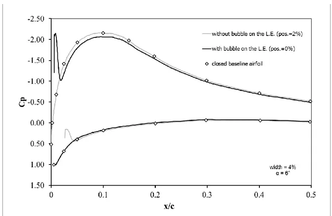
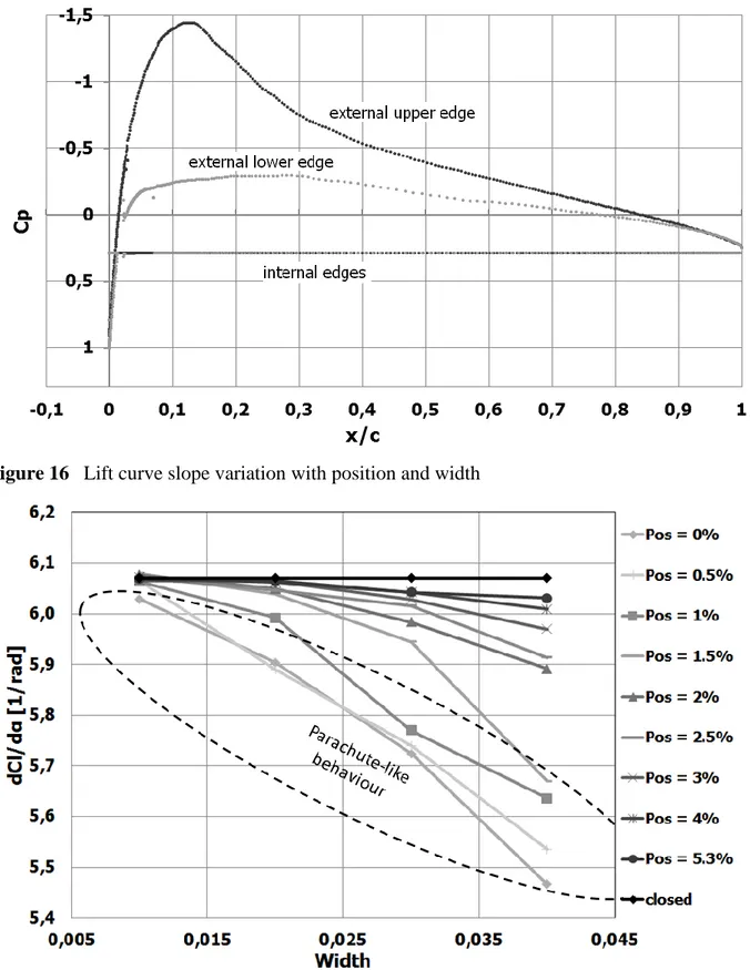
A systematic study shows that the external pressure coefficient curve around the open airfoil is, in every case, mostly equal to that of the baseline airfoil, a difference appears only if a separation bubble occurs near the opening (Figure 12). If it is on the lower edge as in Figure 9c, the curve modification remains in the region of the bubble and is characterized by a local additional depression. If the bubble is on the upper edge as in Figure 9a, there is also a local effect and a global one in addition. This is obvious from a loss at the main depression peak further on the upper side.
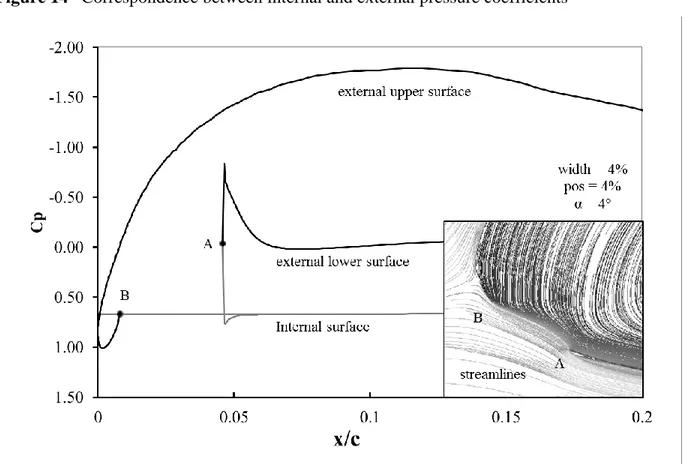
A 3-D mapping of the internal pressure coefficient, with respect to position and width of the air inlet, was performed for an angle of attack of 2° (Figure 13). This angle was evaluated as optimal to describe this phenomenon because it represents, among our studied cases, the most critical for deflation risk due to internal pressure loss. Examining the plot, the influence of the position of the air inlet is essential, while its width represents only a minor contribution to the internal pressure value. The systematic study of pressure coefficient curves correlated with the flow patterns brings a more precise explanation for the way the internal pressure varies. When the stagnation point is located in the air inlet like in Figure 9b, the internal pressure coefficient is maximal with a value of 1. When the stagnation point moves out of the air inlet, the internal pressure is, in all our cases, exactly equal to the external value existing on the edge at the inlet end which is the same side as the external stagnation point (Figure 14). This result is very interesting, as we established previously that the external pressure curve for an open airfoil is nearly the same as that for baseline airfoil. It shows that the internal pressure can be well estimated with only the closed baseline results and the air inlet location.
At present, an absolute quantitative 3D method to evaluate the structural stability of a paraglider regarding the differential pressure between the inner and outer canopy surfaces has
not been established. Indeed, even if the structure can help to maintain the geometry under a local inward pressure balance, the higher the internal pressure, the better the resistance to deflation. So, in our study, Sc1% tends to present an elevated robustness to deflation for every air inlet dimension considered. Internal pressure coefficients decayed rapidly by setting back the air inlet. Increasing the air inlet size partially compensates this loss by enlarging the opening towards the stagnation area. This result confirms that parafoils are more robust to deflation than paragliders because they maintain a high internal pressure at low angles of attack.
This behaviour can be explained by examining the position of the stagnation point for every case. In fact, air inlet positions tailored for gliding parachutes had stagnation points situated either on the location of the air inlet (Figure 9b) or just after on the lower surface (Figure 9a). For this second case, considering that the internal pressure was nearly the same as the one on the edge end between the internal and external fields, the internal pressure coefficient is close to that of the stagnation point. Therefore the internal pressure for parachutes is always equal to, or approaching, Cp = 1. On the other hand, paraglider airfoils can have the stagnation point situated before the air inlet, in the leading edge area, especially if the inlet is located further on the lower surface and the angle of attack is low (Figure 10). This means higher velocities appear on the edge end at the air inlet, therefore causing a decrease in the internal pressure.
In order to focus on a critical case, internal and external surface pressure coefficients plotted versus the relative position to airfoil chord x/c are highlighted for Sc = 3% at the smallest width Sw = 1% and α = 2° (Figure 15). The internal pressure is greater than the external one, except for a small portion close to the leading edge. This condition suggests that the canopy can potentially begin to reverse its curvature locally due to pressure inversion. If this failure extends, the airfoil can be distorted to such an extent, that the frontal collapse limit is reached. Nevertheless, in
modern paragliding industry a solution to delay the problem, such as reinforcing the leading edge with a semi-rigid structure, is often considered. Depending on the type of structure used, some critical configurations become stable. Thus the limit at low angles of attack is extended.
4.4 Influence of the air inlet configuration on lift and drag
Figure 16 shows the lift slope coefficient curves between 2° and 6° for all cases. For small air inlet widths Sw, there is no difference in the slope between the baseline airfoil and the paraglider airfoils. Only when the air inlet is centered at the leading edge can a little gap be noticed. As the width is increased, the difference progressively grows. A more important alteration of the slope clearly appears for some configurations, suggesting two distinct behaviours. At Sw = 2% it concerns Sc0.5%, at Sw = 3% it involves Sc1.0% and at Sw = 4% it concerns Sc1.5%. All these configurations are characterized by an air inlet extending over the beginning of the upper side, just like parafoils. So this first group was named "parachute-like" on the Figure 16. The second group concerns all the other air inlet configurations. They are entirely located on the lower surface of the airfoil and are much "paraglider-like". In the scope of tested parameters values, the degradation of the slope for "parachute-like" is well correlated with the size of the upper separation bubbles growing with the angle of attack as shown in Figure 17. It can be related to the associate loss found at the main depression peak on the upper side suggesting a global effect on the circulation around the airfoil. Inversely, when there is no visible bubble with increasing angle of attack like for Sw = 1% at Sc = 0% (Figure 18), the value of the lifting slope stays similar to that of the baseline. Other local contributions to the lift change, with respect to the baseline airfoil, can be found in the pressure field balance. They derive from the cut part of the airfoil and the depression caused by the separation bubble.
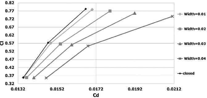
The width effects on polar curves are presented for three air inlet positions, namely Sc = 0% (Figure 19), 2% (Figure 20) and 5.3% (Figure 21). They clearly show different tendencies. At Sc = 0%, thus for a symmetric air inlet, an increase in the width tends to increase the drag a lot and reduce the lift slightly. This effect becomes more pronounced as the angle of attack increases. Sc = 2% stands in contrast, the curves now converge with increasing angles of attack and the lift coefficient Cl rises slightly with the width, especially for low angles of attack. The final position Sc = 5.3%, relatively far downstream, differs from the previous positions with very similar polar curves. There is just, depending on the extent of the width extent, a little additional drag for the closed airfoil case.
For an open airfoil, the aerodynamic force is obtained by the integration of pressure and skin friction on the both sides of the upper and the lower surfaces. Mashud and Umemura (2006) detailed this calculation for the pressure part. Assuming that the internal pressure was uniform, they showed that the result is equal to the integral of the external pressure applied to the upper and lower surfaces, plus the internal pressure applied at the external side of the straight line joining the two inlet extremities.
In order to express this calculation with only the closed baseline airfoil results, another way of decomposition is possible for a paraglider airfoil in its performance range. Applied to the Figure 5 geometry, the pressure integration of the open airfoil is expressed in equation (1). For this kind of performant airfoils, within the range of parameters investigated, there is not a strong separation bubble. Our results show that the external pressure coefficient curve matches very well the baseline airfoil and also that the internal pressure is almost constant. Thus Pext = Pextb
can be used to write equation (2). Adding and subtracting the pressure integration on the both sides of the curve segment corresponding to the air inlet area gives equation (3). As Pint is
constant, its integration around the closed airfoil equals zero and gives equation (4). In the first term, the integration of the external pressure around the baseline airfoil gives its aerodynamic force. In the second term, the integration of the constant pressure Pint on a curve segment is equal
to this pressure applied on the straight line joining its extremities. Finally, the aerodynamic force on the open airfoil is obtained with equation (5). As shown previously, the internal pressure can be deduced from the external pressure field on the baseline airfoil, therefore the force can be evaluated only with baseline airfoil results. This greatly facilitates a quantitative estimation by using published data for closed airfoils or classical airfoil software.
𝐹⃗𝐴 = ∫ (𝑃𝐴𝑇 𝑖𝑛𝑡− 𝑃𝑒𝑥𝑡). 𝑛⃗⃗. 𝑑𝑠+ ∫ (𝑃𝑇𝐵 𝑖𝑛𝑡 − 𝑃𝑒𝑥𝑡). 𝑛⃗⃗. 𝑑𝑠 (1)
𝐹⃗𝐴 = ∫ (𝑃𝐴𝑇 𝑖𝑛𝑡 − 𝑃𝑒𝑥𝑡𝑏). 𝑛⃗⃗. 𝑑𝑠+ ∫ (𝑃𝑇𝐵 𝑖𝑛𝑡− 𝑃𝑒𝑥𝑡𝑏). 𝑛⃗⃗. 𝑑𝑠 (2)
𝐹⃗𝐴 = ∮(𝑃𝑖𝑛𝑡 − 𝑃𝑒𝑥𝑡𝑏). 𝑛⃗⃗. 𝑑𝑠 − ∫ (𝑃𝐵𝐴 𝑖𝑛𝑡− 𝑃𝑒𝑥𝑡𝑏). 𝑛⃗⃗. 𝑑𝑠 (3)
𝐹⃗𝐴 = − ∮ 𝑃𝑒𝑥𝑡𝑏. 𝑛⃗⃗. 𝑑𝑠 − ∫ 𝑃𝐵𝐴 𝑖𝑛𝑡. 𝑛⃗⃗. 𝑑𝑠+ ∫ 𝑃𝐵𝐴 𝑒𝑥𝑡𝑏. 𝑛⃗⃗. 𝑑𝑠 (4)
𝐹⃗𝐴 = 𝐹⃗𝐴𝑏− 𝑃𝑖𝑛𝑡. ‖𝐴𝐵⃗⃗⃗⃗⃗⃗‖. 𝑛⃗⃗ + ∫ 𝑃𝐵𝐴 𝑒𝑥𝑡𝑏. 𝑛⃗⃗. 𝑑𝑠 (5)
Where 𝐹⃗𝐴 is the total aerodynamic force, 𝑛⃗⃗ is a unit outward normal vector, s is the curvilinear abscissa, A is the lower extremity of the air inlet, B is the upper extremity of the air inlet, T is the trailing edge point and b is a subscript for the baseline airfoil.
That decomposition is also an interesting approach to explain the way that the air inlet influences drag and lift. Thus, the additional force on the paraglider airfoil based on the baseline airfoil, is reduced to the localized pressure integration at the air inlet location on the closed baseline airfoil. On the internal side, externals results from the baseline are applied, whereas on the external side the internal pressure from the open paraglider airfoil is used.
When the external pressure field around the air inlet location is almost uniform, it follows from the above that the internal pressure in the paraglider airfoil is also equal to that uniform pressure. So, the integrated pressure is almost the same on the both sides. As a consequence the influence of the air inlet on the pressure force is small and the performance is weakly altered. This situation can arise in two ways: when the air inlet is reduced in size close to the stagnation point or when the air inlet is located downstream on the lower surface. This second case corresponds well to Figure 18. The internal pressure is high in the first case and low in the second, but, in both cases, the influence of the air inlet on the total aerodynamic force is small.
When the stagnation point is just beside the air inlet, an accelerated flow is observed at the inlet location. For this case, it has already been shown that the internal pressure is equal to the external pressure at the extremity A or B of the air inlet which is on the stagnation point side. This internal value is greater than that for the external accelerated flow. So, when evaluating the added force by applying this pressure field on the both sides of the inlet part removed from the baseline airfoil, an extra force appears, directed from the air inlet into the open airfoil. Two subcases must be distinguished. The first one is when the stagnation point is located just after the air inlet on the lower surface, like for gliding parachute airfoil at increasing angle of attack. In front of the air inlet the flow accelerates substantially towards the upper side. Therefore the additional force is significant and oriented mostly backward. This is in correlation with the tendency observed in Figure 19, even though it must be kept in mind that there are also the effects of the separation bubble and the influence of the skin friction. The second subcase arises when the stagnation point is located just before the air inlet in the leading edge area, like for realistic paraglider configurations at low angles of attack, e.g. Sc = 2% and Sw2% at α = 2°. Here the flow accelerates moderately in front of the air inlet, towards the lower surface. The
additional force is moderate and oriented upwards (lift) and backwards (drag). This corresponds well with the remarks made about Figure 20.
4.5 Best configuration
Results are summed up in three 3-D plots where each performance parameter is compared with the result found for the baseline airfoil for α = 6°, representative of a cruise gliding flight.
In Figure 22 the influence of the air inlet configuration on the additional lift coefficient is displayed. When the midpoint of the air inlet is further downstream, a lift coefficient equal or even slightly greater than the value obtained for the baseline airfoil is achieved. On the other hand, as the air inlet midpoint moves upstream, the lift coefficient decreases if the width increases. This is the main effect of the parachute-like behaviour previously noticed.
The influence on drag coefficient (Figure 23) reveals a minimum when Sc = 2%, regardless of its width. Width Sw = 1% and position Sc = 1.5% leads to nearly the same value. When position Sc move below 1.5%, and width Sw is simultaneously increased above 1%, the drag coefficient clearly increases. This is the second aspect denoting a parachute-like behaviour. Its origin is in the previously viewed effect of adding the air inlet contribution in the pressure integration of the baseline airfoil.
The influence on the glide ratio is shown in Figure 24. The observations made for the drag coefficient can be made again here. The efficiency degrades when the position moves towards the leading edge and when the air inlet dimension is increased. As a matter of fact, Sw = 1% and Sc = 2% (Figure 25) was found to be the configuration with the best performance. For the same width, but with Sc = 1.5%, practically the same performance was obtained. These two positions
have in common the total absence of separation bubbles around the air inlet, whatever the angle of attack. In the section 4.3 it was shown that these two configurations fully inflate.
Therefore, the Sw = 1%, Sc = 2% case, was investigated for a wider range of angles of attack, i.e. -4° α 14°, and compared to the baseline airfoil. The drag coefficient for the paraglider airfoil was marginally higher at α0°, slightly lower at α10° and nearly identical elsewhere. The computed lift coefficient was slightly greater than the value calculated for the baseline airfoil at negative angles of attack, practically identical between 0° and 10°, and slightly lower for α greater than 10°. This resulted in two nearly superimposed lift to drag ratio curves.
5 Conclusions
Even if the baseline airfoil used is highly realistic, and representative of a performance paraglider, the results of this study are limited to this shape, at a single Reynolds number, and in the scope of the investigated parameters variations. Under this restriction, it can be concluded that:
The flow pattern reveals one stagnation point when the flow separates in front of the air inlet and two stagnation points when it separates to one side or another. One of these points is always located on the internal side or just at the extremity of one of the air inlet ends. The second stagnation point, when it occurs, is located on the external side of the other air inlet end. When it is located on the internal side, a stagnation point can be associated with a more or less important separation bubble on the external side of the same border. A larger air inlet promotes the development of this separation bubble.
The internal pressure in the airfoil is constant everywhere except near the air inlet. It is equal to the stagnation pressure when the flow separates in front of the air inlet. It decreases when the flow separates to one side of the air inlet, at an external stagnation point. The value of the
internal pressure is equal to the external pressure at the inlet end which is on the same side as the stagnation point.
If there is no separation bubble, the external pressure curve on the open airfoil is the same as for the closed baseline airfoil. For this case, lift and drag of the open paraglider airfoil can be calculated only by knowing the closed baseline airfoil pressure curve, the air inlet location and the value of the internal pressure. From the above conclusion, the internal pressure can also be deduced from the baseline airfoil results. A good approximation is also possible in the same way, for small bubble on the lower surface. These results are important because, generalized to similar airfoils, they give paraglider designers a simple way to obtain a good estimate of the performances and internal pressure with only classical closed airfoil software.
A larger air inlet causes deterioration of the aerodynamic characteristics. A rise in drag is mainly due to a loss of frontal suction in the pressure integration at the air inlet. It is even more important when the air inlet is positioned forward and thus oriented more ahead in an accelerated flow. For a lower amount, the drag increase is also due to the thicker boundary layer obtained when separation bubbles occur.
The association of a large air inlet (>2%) and a forward position (<2%) results in a specific behaviour. It is characterized by a lower lifting curve slope, which originates from the growth of a separation bubble over the leading edge when the angle of attack increases. This affects the whole external pressure curve over the airfoil. Combined with the drag increase, it results in a degraded lift to drag ratio. A position of the air inlet located further downstream leads to less performance alterations, even for large dimensions. Thus, the internal pressure clearly decreases for lower angles of attack. Hence, two clearly separate behaviours for open airfoils are found. The first one is “parachute-like”, with the air inlet acting rather like as a total pressure tap,
resulting in good deflation robustness but performance losses. The second one is “paraglider-like”, at low angles of attack, the air inlet tends to act as a static pressure tap, resulting in less altered performances but lower deflation robustness.
For a paraglider, at a typical cruise angle of attack of α = 6°, the configuration with an air inlet midpoint at 2% and a width of 1% shows the best performances, almost equal to those of the baseline airfoil.
References
Balaji, R., Mittal, S., and Rai, A. K., ‘Effect of Leading Edge Cut on the Aerodynamics of Ram-Air Parachutes,’ International Journal for Numerical Methods in Fluids, Vol. 47, No. 1, 2005, pp. 1-17,.doi:10.1002/fld.779 Burk, S. M., and Ware, G. M., ‘Static Aerodynamic Characteristics of Three Ram-Air Inflated Low Aspect Ratio
Wings,’ NASA TN-D-4182, 1967
Chapin, V., Neyhousser, R., Dulliand, G., and Chassaing, P., ‘Analysis design and optimization of navier-stokes flows around interacting sails’, MDY06 International Symposium on Yacht Design and Production, Madrid, Spain, 30-31 March 2006.
Drela, M., ‘XFOIL: An Analysis and Design System for Low Reynolds Number Airfoils,’ Lecture Notes in Engineering, Vol. 54, 1989, pp 1-12, doi: 10.1007/978-3-642-84010-4_1
Kalitzin, G., ~Medic, G., Iaccarino, G. and Durbin P., ‘Near-wall behaviour of RANS turbulence models and implications for wall functions’ Journal of Computational Physics 204, pp.265-291, 2005,. doi: 10.1016/j.jcp.2004.10.018
Mashud, M., and Umemura A., ‘Experimental Investigations on Aerodynamic Characteristics of a Paraglider Wing,’ Trans. Japan Soc. Aero. Space Sci., Vol. 49, No. 163, pp. 9-17, 2006.
Mashud, M., and Umemura A., ‘Improvement in Aerodynamic Characteristics of a Paraglider Wing Canopy,’ Trans. Japan Soc. Aero. Space Sci. Vol. 49, No. 165, pp. 154-161, 2006
Mittal, S., Saxena, P., and Singh, A., ‘Computation of Two-Dimensional Flows Past Ram-Air Parachutes,’ International Journal for Numerical Methods in Fluids, Vol. 35, No. 6, 2001, pp. 643-667,.doi: 10.1002/1097-0363(20010330)35:6<643::AID-FLD107>3.0.CO; 2-M
Mohammadi, M.A.,Johari, H., ‘Computation of Flow over a High-Performance Parafoil Canopy,’ Journal of Aircraft, Vol. 47, No. 4, 2010, pp. 1338-1345. doi:10.2514/1.47363
Nicolaides, J. D., Speelman, R. J., III, and Menard, G. L. C., ‘A Review of Para-foil Applications,’ Journal of Aircraft, Vol. 7, No. 5, 1970, pp. 423-431, doi:10.2514/3.44194
Ross, J. C., ‘Computational Aerodynamics in the Design and Analysis of Ram-Air-Inflated Wings,’ RAeS/AIAA 12th Aerodynamic Decelerator Systems Technology Conference, AIAA Paper 93-1228, Reston, VA, 1993.
Silva, D., Avelino, M. R. and De-Lemos, M. J. S., ‘Numerical Study of the Airflow around the Airfoil Selig 1223,’ II Congress of Mechanical Engineering, Joao Pessoa, Brazil, August 2002
Spalart, P. R., and Allmaras, S. R., ‘A One-Equation Turbulence Model for Aerodynamic Flows’, AIAA Paper 92-0439, Jan. 1992, doi: 10.2514/6.1992-439
Tribot, J.-P., Rapuc, M., and Durand, G., ‘Large Gliding Parachute Experimental and Theoretical Approaches,’ 14th AIAA Aerodynamic Decelerator Systems Technology Conference, AIAA Paper 97-1482, Reston, VA, 1997, doi: 10.2514/6.1997-1482
Ware, G. M., and Hassell, J. L., ‘Wind Tunnel Investigations of Ram-Air Inflated All-Flexible Wings of Aspect ratio 1.0 to 3.0,’ NASA TMSX-1923, 1969.
Figure 2 Mesh produced for Sw = 2% and Sc = 2% a) around the whole airfoil, b) focused on
the air inlet region
a),
Figure 3 Lift curve for the baseline airfoil
Figure 5 Definition of air inlet geometry
Figure 7 Vorticity contours for the baseline airfoil
Figure 8 Turbulent viscosity ratio inside and around the open airfoil
Figure 9 Streamlines at α = 6° for three different configurations:
a) Sc = 0% Sw = 3%, b) Sc = 2% Sw = 4%, c) Sc = 4% Sw = 4%
Figure 10 Streamlines at α = 4° for Sc = 5.3%, Sw = 4%
Figure 12 Comparison of closed airfoil and open airfoil pressure coefficient curves
Figure 15 Cp values for a critical internal pressure case at α = 2°, Sw = 1% and Sc = 3%
Figure 17 Streamlines for Sc = 0%, Sw = 4% and varying α : a) 2°, b) 4° and c) 6°
a), b), c),
Figure 18 Streamlines for Sc = 0%, Sw = 1% and varying α : a) 2°, b) 4° and c) 6°
a), b), c),
Figure 20 Polar for four widths positioned at Sc = 2%
Figure 22 Change in Cl for α = 6° relative to the baseline airfoil as a function of Sc and Sw
Figure 24 Change in glide ratio for α = 6° relative to the baseline airfoil as a function of Sc and
Sw
Figure 25 Streamlines at α = 6° for the combination yielding the best performance: Sc = 2%,