Adaptive detection of a Gaussian signal in Gaussian noise

(1)

Any correspondence concerning this service should be sent to the repository

administrator:

staff-oatao@listes-diff.inp-toulouse.fr

O

pen

A

rchive

T

OULOUSE

A

rchive

O

uverte (

OATAO

)

OATAO is an open access repository that collects the work of Toulouse researchers and

makes it freely available over the web where possible.

This is an author-deposited version published in:

http://oatao.univ-toulouse.fr/

Eprints ID: 16661

To cite this version:

Besson, Olivier and Chaumette, Eric and Vincent, François Adaptive

detection of a Gaussian signal in Gaussian noise. (2016) In: CAMSAP 2015, 13

December 2015 - 16 December 2015 (Cancun, Mexico).

(2)

Adaptive detection of a Gaussian signal in Gaussian

noise

Olivier Besson, Eric Chaumette and Franc¸ois Vincent

University of Toulouse, ISAE-Supa´ero

Department of Electronics, Optronics and Signal 10 Avenue Edouard Belin, 31055 Toulouse France

Abstract—Adaptive detection of a Swerling I-II type target in Gaussian noise with unknown covariance matrix is addressed in this paper. The most celebrated approach to this problem is Kelly’s generalized likelihood ratio test (GLRT), derived under the hypothesis of deterministic target amplitudes. While this conditional model is ubiquitous, we investigate here the equivalent GLR approach for an unconditional model where the target amplitudes are treated as Gaussian random variables at the design of the detector. The GLRT is derived which is shown to be the product of Kelly’s GLRT and a corrective, data dependent, term. Numerical simulations are provided to compare the two approaches.

I. PROBLEM FORMULATION

Thirty years ago, in a series of technical reports and pa-pers now became classic references [1]–[5], Kelly thoroughly investigated the problem of detecting a signal of interest (SoI) buried in Gaussian noise with unknown covariance matrix. This problem can be formulated as the following composite binary hypothesis test

H0: ⇢ xtp= ntp; tp = 1,· · · , Tp yts= nts; ts= 1,· · · , Ts H1: ⇢_x tp= ↵tpv + ntp; tp= 1,· · · , Tp yts= nts; ts= 1,· · · , Ts (1) where X = ⇥x1 · · · xTp ⇤

2 CM⇥Tp stands for the

observation matrix where the presence of a signal of interest is sought. The latter has (unit-norm) known signature v and

its complex amplitude is ↵tp. The data matrix X is often

referred to as the primary data. ntpcorresponds to the additive noise, which is assumed to be zero-mean, complex Gaussian distributed with unknown positive definite covariance matrix

R 2 CM⇥M_{, which we denote as n}

tp ⇠ CN (0, R).

Additionally, it is assumed that Tssnapshots yts are available, which contain noise only, i.e., yts are independent, zero-mean

complex Gaussian vectors drawn from yts⇠ CN (0, R).

The problem in (1) arises in many fields of engineering, and is particularly important for radar applications. In the latter case, the matrix X corresponds to the radar returns at the range cells under test (CUT), v is the target space or time or space-time signature, and ytsare radar data collected in range cells in the vicinity of the CUT [4]. The most usual case corresponds

to a single CUT for which Tp = 1, while the case Tp > 1

is related to the detection of a range spread target [6] or to the detection over multiple coherent processing intervals. The reference approach to solve this problem is Kelly’s generalized likelihood ratio test (GLRT) [1], [4], which was obtained under

the assumption that ↵tp are unknown deterministic quantities. Kelly’s GLRT takes the following form:

GLR1/Tt c = |I + XH_S 1 y X| |I + XHSy1/2P?_S 1/2 y vS 1/2 y X| (2)

where Tt = Tp+ Ts, Sy = Y YH is Ts times the sample

covariance matrix of the secondary data Y =⇥y1 . . . yts ⇤

,

P?

Sy1/2v denotes the orthogonal projector onto the subspace

orthogonal to S 1/2

y v, and |.| stands for the determinant of

a matrix. Kelly provided a detailed statistical analysis of this detector both in the case of matched or mismatched signature

[2], [5]. Under the same assumption and in the case Tp = 1,

Robey et al. derived the adaptive matched filter in [7]. This is indeed a two step GLRT where at the first step R is assumed to be known (and the GLR is derived from X only), and at

the second step T 1

s Sy is substituted for R.

Surprisingly enough, considering ↵tp as a random variable has received little attention, and the quasi totality of recent studies followed the lead of [4] and considered ↵tp as deter-ministic parameters. Although the literature on the topic cannot be browsed exhaustively, we are not aware of references that would address detection of a Gaussian signal in colored noise with unknown covariance matrix (while the case of white noise has been examined thoroughly). In [8], detection of an arbitrary Gaussian signal is addressed but this signal is not aligned on a known signature. The advantages of a “conditional” model are that 1)one does not formulate any assumption on the amplitude statistics and 2)derivations involve a simple linear least-squares

problem with respect to ↵tp. One drawback might be that

the number of unknowns grows with Tp and, therefore, an

unconditional model is worthy of investigation. Moreover, a stochastic assumption for ↵tpmakes sense. Indeed, we assume

herein that ↵tp are independent and drawn from a complex

Gaussian distribution with zero mean and unknown variance

P, i.e., ↵tp ⇠ CN (0, P ), which complies with the widely

accepted Swerling I-II target model [9], [10]. The problem in (1) can thus be re-formulated as

H0:X ⇠ CN 0, R, ITp ; Y ⇠ CN (0, R, ITs)

H1:X ⇠ CN 0, R + P vvH, ITp ; Y ⇠ CN (0, R, ITs) .

(3) The main difference with the deterministic approach is that,

under H1, the SoI is embedded in the covariance matrix of X

instead of in its mean value.

The aim of this paper is to provide answers to the following questions:

(3)

1) is it possible to derive the GLRT for the problem in (3)?

2) if so, does it result in any improvement compared to

(2)?

II. GENERALIZED LIKELIHOOD RATIO TEST

In this section, we derive the GLRT for the problem de-scribed in (3) and relate it to Kelly’s GLRT in the deterministic case. Since both P and R are unknown, the GLR in this case writes max P,R p1(X, Y ) max R p0(X, Y ) (4)

where p`(X, X) is the probability density function of the

observations under hypothesis H`.

Under H0 the p.d.f. of the observations is given by

p0(X, Y )/ |R| Ttetr

n

R 1⇣Sy+ XXH

⌘o (5) where etr {.} stands the exponential of the trace of a ma-trix and / means proportional to. In this case, it is well

known that the maximum of p0(X, Y ) is achieved for R =

Tt 1

⇣

Sy+ XXH

⌘

and is thus given by max

R p0(X, Y )/ |Sy+ XX

H

| Tt_. (6)

Under H1, let V = [v V?] be a unitary matrix, with

V_? a basis for the subspace orthogonal to v, i.e., VH

?v = 0

and VH

?V? = IM 1. This transformation brings v to

VHv = e1= [1 0 · · · 0]

T

. Let us define the transformed

data ˜X = VHX = _˜ X1 ˜ X2 and ˜Y = VHX = _˜ Y1 ˜ Y2 , and

transformed covariance matrix ˜R = VHRV. The joint p.d.f.

of X and Y can be expressed as p1(X, Y )/ | ˜R| Ts| ˜R + P e1eH1| Tp ⇥ etrn R˜ 1Y ˜˜YHoetrn ( ˜R + P e1eH1) 1X ˜˜X Ho . (7) Let us decompose ˜Ras ˜ R = ✓_˜ R11 R˜12 ˜ R21 R˜22 ◆ (8) and let ˜R1.2 = ˜R11 R˜12R˜ 1 22R˜21and = ˜R 1 22R˜21. Observe

that ˜Rcan be equivalently parametrized by ( ˜R11, ˜R21, ˜R22)

or ( ˜R1.2, , ˜R22). Using the facts that | ˜R| = ˜R1.2| ˜R22| and

˜ R 1= ˜R_1.21 ✓ 1 H H ◆ + ✓₀ ₀ 0 R˜221 ◆ (9) one can rewrite (7) as

p1(X, Y )/ | ˜R22| TtR˜1.2Ts ⇣ P + ˜R1.2 ⌘ Tp ⇥ etrn R˜221 ⇣ ˜ Y2Y˜ H 2 + ˜X2X˜ H 2 ⌘o ⇥ exp ⇢ _⇥ 1 H⇤ ˜A  1 ₍₁₀₎

where we temporarily define ˜ A = ˜R1.21S˜y+ ⇣ P + ˜R1.2 ⌘ 1 ˜ X ˜XH. (11) Since ⇥ 1 H⇤ ˜A  1 =⇣ A˜221A˜21 ⌘H ˜ A22 ⇣ ˜ A221A˜21 ⌘ + ˜A11 A˜12A˜ 1 22A˜21 (12) it follows that p1(X, Y )/ | ˜R22| Ttetr n ˜ R₂₂1⇣Y˜2Y˜ H 2 + ˜X2X˜ H 2 ⌘o ⇥ exp⇢ ⇣ A˜221A˜21 ⌘H ˜ A22 ⇣ ˜ A221A˜21 ⌘ ⇥ ˜R Ts 1.2 ⇣ P + ˜R1.2 ⌘ Tp expn A˜1.2 o . (13)

Clearly, p1(X, Y ) is maximized for R˜22 =

Tt 1 ⇣ ˜ Y2Y˜ H 2 + ˜X2X˜ H 2 ⌘ , = A˜221A˜21, which results in max ˜ R22, p1(X, Y )/ | ˜Y2Y˜ H 2 + ˜X2X˜ H 2| Tt ⇥ ˜R Ts 1.2 ⇣ P + ˜R1.2 ⌘ Tp expn A˜1.2 o . (14)

Next, observe that ˜A_1.21 is the upper-left corner of ˜A 1 and the latter is given by

˜ A 1= ˜R1.2 h ˜ Sy+ (1 + P ˜R1.21) 1X ˜˜X Hi 1 = ˜R1.2VH h Sy+ (1 + P ˜R1.21) 1XX Hi 1_{V .} ₍₁₅₎ It ensues that ˜ A_1.21= ˜R1.2vH h Sy+ (1 + P ˜R1.21) 1_XXHi 1_v. ₍₁₆₎

For the sake of notational convenience, let us introduce a = ˜R1.2 and b = P ˜R1.21. Observe that b = P vHR 1v is

tantamount the signal to noise ratio at the output of the optimal filter R 1_{v. Then, one can rewrite (14) as}

max ˜ R22, p1(X, Y )/ |VH_? ⇣ Sy+ XXH ⌘ V?| Tt ⇥ a Tt_{(1 + b)} Tp ⇥ exp ( a 1  vH⇣_S y+ (1 + b) 1XXH ⌘ 1 v 1) . (17) Using the readily verified facts that

max a a Tt_exp _⇠ 1_a 1 ₌ ✓ _e Tt ◆ Tt ⇠Tt (18) along with |VH ? ⇣ Sy+ XXH ⌘ V?| = vHSy1v ⇥ |Sy||I + XHSy1/2P?_S 1/2 y vS 1/2 y X| (19)

(4)

we get that max ˜ R22, ,a p1(X, Y )/ |Sy| Tt ⇥ |I + XHSy1/2P?_S 1/2 y vS 1/2 y X| Tt ⇥ (1 + b) Tp 2 6 4 vH⇣_S y+ (1 + b) 1XXH ⌘ 1 v vH_S 1 y v 3 7 5 Tt . (20) It is possible to show that the term in the last line can be equivalently written as vH⇣_S y+ (1 + b) 1XXH ⌘ 1 v vH_S 1 y v = |I + (1 + b) 1_XH_S 1/2 y P?_S 1/2 y vS 1/2 y X| |I + (1 + b) 1_XH_S 1 y X| . (21)

Finally, the GLR for Gaussian signals is given by

The first term of the product is recognized as Kelly’s test statistic, i.e., the GLR for deterministic amplitudes ↵tp. The second term (which is always lower than one) is a corrective term due to the fact that now ↵tp are considered as Gaussian distributed random variables.

Remark 1. Since the above GLR involves the same quantities as Kelly’s GLR, it follows that is has a constant false alarm rate with respect to R, i.e., its distribution under H0is independent

of R.

Remark 2. The new detector involves additional computations compared to Kelly’s detector due to the need to solve the optimization problem in (22). However, the extra cost is not

that large. Let us define ⌘ = (1 + b) 1

2 [0, 1] and Sxy =

Sy+ XXH. Then, if the determinant form is employed, one

can make use of the fact that |I + ⌘M| = Q[1 + ⌘ j(M )]

where j(M )are the eigenvalues of M, to efficiently compute

the function to be maximized with respect to ⌘. Likewise, if the second form of the detector is used, one can notice that

f (⌘) = vH⇣Sy+ ⌘XXH ⌘ 1 v = vH⇣Sxy+ (⌘ 1)XXH ⌘ 1 v = vH_S 1 xyv (⌘ 1)vHSxy1X h ITp+ (⌘ 1)X H_S 1 xyX i 1 XHS_xy1v (23)

which can be used, e.g., to compute efficiently f(⌘) over a grid of values of ⌘ and solve the optimization problem.

III. NUMERICAL SIMULATIONS

We now provide numerical illustrations of the performance of the new detector and compare it with Kelly’s GLRT. We consider a radar scenario with M = 16 pulses. The SoI signature is given by v = ⇥1 ei2⇡fs _{. . .} _ei2⇡(M 1)fs⇤T with fs = 0.09. The noise vectors ntp and nts include both thermal noise and clutter components, which are assumed to be uncorrelated so that R = Rc+ 2nI. The clutter covariance

ma-trix is selected as [Rc]m1,m2 / exp n

2⇡2 2

f(m1 m2)2

o

with 2

f = 0.01. The clutter to white noise ratio (CWNR)

is defined as CW NR = Tr{Rc}/Tr{ n2I} and is set to

CW N R = 20dB in the simulations. The signal to noise ratio

is defined as SNR = P vH_R 1_{v. The probability of false}

alarm is set to Pf a = 10 3.

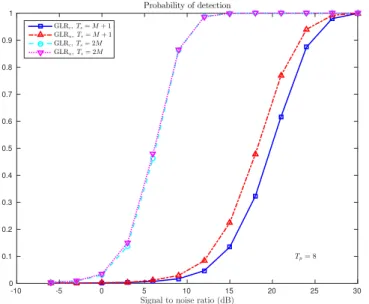
In Figures 1-2 we provide an excerpt of the results

ob-tained. The main conclusions are the following. When Tp= 1,

the two detectors provide the same probability of detection,

whatever Ts. Differences can only be observed when Tp =

4, 8, and Ts is small, typically Ts= M + 1, see Figures 1-2.

In this case, the new detector provides improvement compared

to Kelly’s detector. Otherwise, even when Tp = 4, 8 and

Ts= 2M, the two detectors behave the same. Note that we did

not observe scenarios where the new detector would perform worst than Kelly’s GLRT.

Signal to noise ratio (dB)

-10 -5 0 5 10 15 20 25 30 0 0.1 0.2 0.3 0.4 0.5 0.6 0.7 0.8 0.9 1 Tp= 4 Probability of detection GLRc, Ts= M + 1 GLRu, Ts= M + 1 GLRc, Ts= 2M GLRu, Ts= 2M

Fig. 1. Probability of detection versus SNR. M = 16 and Tp= 4.

IV. CONCLUSIONS

In this paper, we revisited the classical problem of detecting a signal of interest in colored Gaussian noise with unknown covariance matrix. The chief systematic approach is to follow Kelly’s lead and use the GLRT based on deterministic signal amplitudes (conditional model). Herein, we took a different path and investigated whether it was possible to derive the GLRT assuming Gaussian signal amplitudes (unconditional model). It proved to be possible and an expression for the GLRT was derived, which bears some resemblance with Kelly’s GLRT. The new detector was shown to improve over Kelly’s only when the number of primary data is not small

(5)

Signal to noise ratio (dB) -10 -5 0 5 10 15 20 25 30 0 0.1 0.2 0.3 0.4 0.5 0.6 0.7 0.8 0.9 1 Tp= 8 Probability of detection GLRc, Ts= M + 1 GLRu, Ts= M + 1 GLRc, Ts= 2M GLRu, Ts= 2M

Fig. 2. Probability of detection versus SNR. M = 16 and Tp= 8. while the number of secondary data is small. Otherwise the two detectors offer the same performance.

ACKNOWLEDGMENT

This work is partly supported by DGA/MRIS under grant no. 2015.60.0090.00.470.75.01.

APPENDIX

Similarly to [7], let us investigate a two-step approach where, at the first step, we assume that R is known. Then, one has p1(X)/ |R + P vvH| Tpetr n XH R + P vvH 1Xo = p0(X) 1 + P vHR 1v Tp exp ⇢_{P v}H_R 1_S xR 1v 1 + P vH_R 1_v . (24)

where Sx = XXH. Let u = vHR 1v and v =

vH_R 1_S

xR 1v. Some simple calculations enable one to

prove that max P p1(X) p0(X) = 8 < : 1 v_{ uT}p ⇣ v uTp ⌘ Tp expnTp ⇣ v uTp 1 ⌘o v > uTp. (25) Let g(x) = x Tp_exp_{(x _1)T

p} and u(.) denote the

unit-step function, i.e., u(x) = 1 for x > 0, and 0 if x < 0. Then, the GLRT for known R is given by

GLRT_|R(X) = 1 +  g ✓_vH_R 1_S xR 1v (vH_R 1_v)T p ◆ 1 ⇥ u ✓_vH_R 1_S xR 1v (vH_R 1_v)T p 1 ◆ . (26)

In order to make the detector adaptive, `a la AMF, T 1

s Sy

should be substituted for R in the previous equation.

REFERENCES

[1] E. J. Kelly, “Adaptive detection in non-stationary interference, Part I and Part II,” Massachusetts Institute of Technology, Lincoln Laboratory, Lexington, MA, Tech. Rep. 724, June 1985.

[2] ——, “Adaptive detection in non-stationary interference, Part III,” Massachusetts Institute of Technology, Lincoln Laboratory, Lexington, MA, Tech. Rep. 761, 24 August 1987.

[3] E. J. Kelly and K. M. Forsythe, “Adaptive detection and parameter estimation for multidimensional signal models,” Massachusetts Institute of Technology, Lincoln Laboratory, Lexington, MA, Tech. Rep. 848, April 1989.

[4] E. J. Kelly, “An adaptive detection algorithm,” IEEE Transactions Aerospace Electronic Systems, vol. 22, no. 1, pp. 115–127, March 1986. [5] ——, “Performance of an adaptive detection algorithm; rejection of unwanted signals,” IEEE Transactions Aerospace Electronic Systems, vol. 25, no. 2, pp. 122–133, April 1989.

[6] E. Conte, A. De Maio, and G. Ricci, “GLRT-based adaptive detection algorithm for range-spread targets,” IEEE Transactions Signal Process-ing, vol. 49, no. 7, pp. 1336–1348, July 2001.

[7] F. C. Robey, D. R. Fuhrmann, E. J. Kelly, and R. Nitzberg, “A CFAR adaptive matched filter detector,” IEEE Transactions Aerospace Electronic Systems, vol. 28, no. 1, pp. 208–216, January 1992. [8] R. S. Raghavan, H. F. Qiu, and D. J. McLaughlin, “CFAR detection

in clutter with unknown correlation properties,” IEEE Transactions Aerospace Electronic Systems, vol. 31, no. 2, pp. 647–657, April 1995. [9] P. Swerling, “Probability of detection for fluctuating targets,” IRE Transactions Information Theory, vol. 6, no. 2, pp. 269–308, April 1960. [10] ——, “Radar probability of detection for some additional fluctuating target cases,” IEEE Transactions Aerospace Electronic Systems, vol. 33, no. 2, pp. 698–709, April 1997.